Evaluation of Models for Forecasting Daily Foreign Exchange Rates Between Nigerian Naira and US Dollar Amidst Volatility

95

International Journal of Science and Business

Published By

Evaluation of Models for Forecasting

Daily Foreign Exchange Rates

Between Nigerian Naira and US

Dollar Amidst Volatility

Maigana Alhaji Bakawu, Ahmed Abdulkadir, Shafiu Usman Maitoro & Abdulrahman Malik

Abstract

In her quest to put the nations’ foreign exchange policy in line with global practice, the Central Bank of Nigeria (CBN) in the mid of 2016 made a paradigm shift by unveiling flexible foreign exchange policy driven purely by market forces. Consequently, forecasting models reported during pegging policy era may be deeming obsolete. This paper proposed a prediction model for future daily selling exchange rate between Nigerian Naira and United States Dollar in the interbank market amidst volatility using daily rates made available by the Central Bank of Nigeria over the periods July, 2016 to October, 2017. We applied the Box-Jenkins methodology to the Naira – US Dollar exchange rate series in order to build an adequate and well specified prediction model. On the first phase of the study, we checked the stationarity of the series and based on Augmented Dickey-Fuller test and correlogram, the series is stationary at level. The findings revealed that the future daily exchange rate of Naira per US Dollar depends on its past rates and associated innovations. This is evident from the fact that turned out parsimonious model for forecasting the parity between the two currencies on the basis of Bayesian Information Criterion. The said model yielded error of forecast (MAPE) within ten percent.

IJSB

Accepted 05 January 2020 Published 08 January 2020 DOI: 10.5281/zenodo.3601100

Keywords: Autoregressive, Box-Jenkin’s Methodology, Exchange Rates, Moving Average, Naira, United States Dollar.

Volume: 4, Issue: 1 Page: 95-105

2020

ISSN 2520-4750 (Online) & ISSN 2521-3040 (Print)

International Journal of Science and Business

Maigana Alhaji Bakawu, (Corresponding Author), Department of Statistics, Mai Idris Alooma Polytechnic Geidam, Nigeria.

Ahmed Abdulkadir, Department of Mathematical Sciences, Abubakar Tafawa Balewa University Bauchi, Nigeria.

Shafiu Usman Maitoro, Department of Statistics, Abubakar Tatari Ali Polytechnic Bauchi, Nigeria.

Abdulrahman Malik, Department of Statistics, Mai Idris Alooma Polytechnic Geidam, Nigeria.

96

International Journal of Science and Business

Published By 1. Introduction

The central bank of Nigeria in the mid of 2016 in a change of tack allow the Naira to float after declining growth consecutively seen for two quarters. This change of tack put Nigeria in line with most central banks, including the Bank of England and the Naira likely to plunge when the system starts (Laessing & Brock, 2016). In line with this speculation, the parity between the Nigerian Naira (NGN) and the United States Dollar (USD) now stood at 300-odd Naira opposed to N197 per US Dollar in the interbank market amounting to the view that in the modern world, exchange rates of the most successful countries are tends to be floating (Sullivan, 2001). This volatility has received attention of many researchers in the recent times as (Brownlees, Engle, & Kelly, 2011) reported that volatility modeling has been one of the most active financial time series research areas in the past decade. Given the uncertainty and risk associated with volatile exchange rates as well as the frequent exchange rate policy changes in many developing countries, there is need to measure exchange rate volatility across time (Emenike, 2016). Foreign Exchange (Forex) is a type of transaction where a party obtains some units in one currency to buy proportion amount in another currency (Sidehabi, et al, 2016). This exchange is usually conducted in pair currency. The most popular pair and trade worldwide is Euro vs. USD (EUR / USD). In Nigeria, the most popular pair and trade is Naira – United States Dollar, because according to (Central Bank of Nigeria, 2016), the dollar is the intervention currency in the market; while the exchange rates of other currencies are based on cross reference to the naira - dollar exchange rates.

Forecasting models reported during pegging policy era may be deeming obsolete with the unveiling of this flexible foreign exchange policy driven purely by market forces, since the parity is no longer pegged. Hence, this paper aimed to propose a basic framework for forecasting and understanding the future daily exchange rate dynamics between Nigerian Naira and United States Dollar in the interbank market amidst volatility.

2. Review of Literature

97

International Journal of Science and Business

Published By

Omani Rial, Qatari Riyal, Saudi Arabian Riyal, Somali Shilling, Syrian Pound, Tunisian Dinar and Yemeni Rial, all against the US Dollar as cited by (Emenike, 2016). Additionally, in their paper titled “Forecasting Exchange rate between the Ghana Cedi and the US dollar using time series analysis” (Appiah & Adetunde, 2011) discovered that ARIMA (1, 1, 1) was the best model for Ghana’s cedi against US dollar and a forecast for two years were made from January 2011 to December 2012. Their findings also revealed that predicted rates were consistent with the depreciating trend of the series. Nevertheless, the literature on Naira – US Dollar exchange rates prediction modeling could not be exceptional from the claim: there are lots of works done on time series based on prediction modeling of foreign currency rates in literature as noted earlier. This is defensible as number of researchers have reported different models for predicting exchange rates between Naira and US Dollar. On a similar note, (Nwankwo, 2014) discovered that residuals is negligible when ARIMA (1 0 0) identified as the model that best fit the average yearly exchange rates for US Dollar in Naira for the period 1992 to 2011. Likewise, (Onasanya & Adeniji, 2013) found that for the period January 1994 to December 2011, ARIMA (1, 2, 1) is the best model that explains the NGN/USD exchange rates. The results of their findings further uncovered that the error is white noise and presence of no serial correlation, thus confirming the suitability of the model for forecasting. In a related work, a comparison of Central Bank of Nigeria exchange rates, Bureau de Change rates and Inter-bank exchange rates over a period of thirty-five years by (Mojekwu, et al, 2011) reveals that there are variations in modes of monetary exchange rates against US Dollars in Nigeria. The study uses Autoregressive integrated moving average model to fit time series to the three sets of data.

With the unveiling of the flexible foreign exchange policy driven purely by market forces by the Central Bank of Nigeria in the mid of 2016 and the consequent volatility in the nation’s Forex market, forecasting models reported by number of authors like (Emenike, 2016) (Nwankwo, 2014) and (Onasanya & Adeniji, 2013) among others during pegging policy era may be deeming obsolete since the parity is no longer pegged. Hence the need for a basic framework for forecasting and understanding the future daily exchange rate dynamics between Nigerian Naira and United States Dollar amidst volatility.

3. Objectives

The general objective of the paper is to propose a prediction model for future daily exchange rates between Naira and US Dollar. The specific objectives are to:

a) select a parsimonious model for predicting daily parity between Naira and US Dollar. b) determine the adequacy of the selected model based on model diagnostics tools.

c) evaluate the effectiveness of the model considered on the basis of performance metrics

4. Methodology

In order to achieve the aim of this study, we adopt the notion introduced by Box and Jenkins (1976). The notion is also known as , specifically, the three parameters in the model are: the autoregressive parameter (p), the number of differencing passes (d), and moving average parameter (q) (Indrabayu, et al, 2013). ARIMA is used to predict a value in a response time series as a linear combination of its own past values and past innovations. The general form of the ARIMA model of order p, d and q is presented as follows:

98

International Journal of Science and Business

Published By

Where (difference operator) Difference dimension

Response variable at time t Innovation term at time t

Lag operator; generally while,

Are respectively p and q-order polynomials in the lag operator.

The Naira-US Dollar ARIMA modeling methodology is categorically divided into three, as (Abdullah, 2012) reported that ARIMA model for any variable involves primarily three steps: identification, estimation and diagnostic checking. Thus, these three steps are now explained for the Nigerian Naira – United States Dollar Selling Exchange Rates forecasting model.

4.1.Model Identification

The first phase of ARIMA modelling is the identification of the number of differencing passes (d) and the proper orders of AR and MA parameters (p and q respectively) for the model. However, this can only be achieved if the series is stationary, stationarity can be assessed by either Augmented Dickey – Fuller (ADF) test, runs sequence plot or correlogram.

4.1.1 Stationarity. In order to build an adequate and well specified Naira – US Dollar exchange rates forecasting model, we subjected the series to stationarity test using Augmented Dickey – Fuller (ADF) Test along with runs sequence plot and correlogram. The ADF test the existence of unit root in the exchange rate series and it is also important in determining whether the model to be identified contains constant term. Computational formula of Dickey – Fuller Test is as follows:

(a)

The testing procedure for the ADF test is the same as for the Dickey–Fuller test but it is

applied to the model:

(b)

The unit root test is then carried out under the null hypothesis against the alternative

hypothesis of . Once a value for the test statistics computed, it can be compared to the

relevant critical value for the Dickey–Fuller Test.

Where Estimated autocorrelation of the series at lag k. The statement of the hypotheses is as follows:

Ho: The Naira – US Dollar Exchange Rate series have unit root.

H1: The Naira – US Dollar Exchange Rate series does not have unit root.

While the mathematical form of the Autocorrelation Function (ACF) and Partial Autocorrelation Function (PACF) are respectively given in (c) and (d):

(c)

(d)

Where:

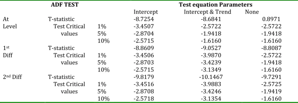
From the summary of the Augmented Dickey- Fuller Test (Table 1), it is apparent that the Naira – US Dollar exchange rates series is stationary at level, first difference (1st _{Diff) and}

second difference (2nd _{Diff) as it can be seen that ADF Statistics are less than the test critical}

99

International Journal of Science and Business

Published By

Table 1. ADF unit root test summary at different form

ADF TEST Test equation Parameters

Intercept Intercept & Trend None

At

Level T-statistic Test Critical -8.7254 -8.6841 0.8971

values 1% 5% -3.4507 -2.8704 -2.5722 -1.9418 -2.5722 -1.9418

10% -2.5715 -1.6160 -1.6160

1st

Diff T-statistic Test Critical -8.8609 -9.0527 -8.8087

values 1% 5% -3.4506 -2.8703 -3.9870 -3.4239 -2.5722 -1.9418

10% -2.5715 -3.1349 -1.6160

2nd _{Diff T-statistic -9.8179 -10.1467 -9.7291}

Test Critical

values 1% 5% -3.4516 -2.8708 -3.9883 -3.4246 -2.5725 -1.9419

10% -2.5718 -3.1354 -1.6160

The result of the ADF test is further consolidated by the runs sequence plot (Figure 1) and correlogram of the series (Figure 2). It is obvious that the pattern of the runs sequence plot contains neither time variant trend nor seasonal cycles and both Autocorrelation (AC) Function and Partial Autocorrelation (PAC) Function plots rapidly decayed to zero as depicted by Figure 1 and 2 respectively. Additionally, it could be deduced from the appearance of the AC and PAC Function plots that mixed model is likely to best fit the series.

280 290 300 310 320 330

25 50 75 100 125 150 175 200 225 250 275 300 325

E x c h a n g e R a te s Index

Figure 1. Runs sequence plot of naira-us dollar exchange rates

Autocorrelation Partial Correlation AC PAC Q-Stat Prob 1 0.865 0.865 245.68 0.000 2 0.775 0.103 443.17 0.000 3 0.682-0.033 596.82 0.000 4 0.585-0.074 709.97 0.000 5 0.490-0.056 789.62 0.000 6 0.411 0.003 845.85 0.000 7 0.281-0.246 872.20 0.000 8 0.189 0.006 884.19 0.000 9 0.106-0.013 887.95 0.000 10 0.029-0.024 888.24 0.000 11-0.061 -0.132 889.50 0.000 12-0.146 -0.107 896.74 0.000 13-0.196 0.103 909.78 0.000 14-0.224 0.032 926.87 0.000 15-0.226 0.072 944.41 0.000 16-0.200 0.104 958.21 0.000 17-0.213 -0.119 973.83 0.000 18-0.216 -0.046 990.03 0.000 19-0.234 -0.172 1009.0 0.000 20-0.255 -0.092 1031.6 0.000 21-0.248 0.059 1053.1 0.000 22-0.240 -0.019 1073.3 0.000 23-0.227 0.065 1091.5 0.000 24-0.220 -0.085 1108.6 0.000 25-0.219 -0.050 1125.6 0.000 26-0.166 0.212 1135.4 0.000 27-0.152 -0.116 1143.6 0.000 28-0.138 0.037 1150.4 0.000 29-0.121 -0.025 1155.6 0.000 30-0.104 0.019 1159.5 0.000 31-0.088 -0.040 1162.3 0.000 32-0.010 0.089 1162.4 0.000 33-0.000 -0.105 1162.4 0.000 34-0.000 -0.137 1162.4 0.000 35 0.001 0.009 1162.4 0.000 36 0.001-0.008 1162.4 0.000

Figure 2: correlogram of the naira –us dollar exchange rate

100

International Journal of Science and Business

Published By

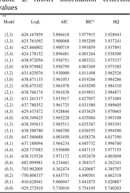
values and forecasted rates of the 25 models are presented in Figure 3 and Figure 4 respectively using simple Bar Chart and runs sequence plot to further highlight the selection justification of the orders of the Autoregressive (AR) and the Moving Average (MA) models. Table 2. ARMA information criterion

values

Model LogL AIC BIC* HQ

(2,3) -626.167859 3.896418 3.977915 3.928943

(3,3) -625.761092 3.900068 3.993209 3.937241

(2,4) -625.866802 3.900719 3.993859 3.937891

(3,4) -624.178152 3.896481 4.001264 3.938300

(1,1) -638.972056 3.956751 4.003321 3.975337

(2,0) -638.979882 3.956799 4.003369 3.975385

(3,2) -631.625076 3.930000 4.011498 3.962526

(3,0) -638.671133 3.961053 4.019266 3.984286

(1,2) -638.675102 3.961078 4.019290 3.984310

(2,1) -638.766174 3.961638 4.019851 3.984871

(4,2) -631.261517 3.933917 4.027057 3.971089

(2,2) -637.780352 3.961725 4.031580 3.989605

(4,3) -629.437472 3.928846 4.033629 3.970665

(4,0) -638.349625 3.965228 4.035084 3.993108

(1,3) -638.395613 3.965511 4.035367 3.993391

(3,1) -638.588780 3.966700 4.036555 3.994580

(1,0) -647.560688 4.003450 4.038378 4.017390

(4,1) -637.188094 3.964234 4.045732 3.996760

(4,4) -628.737083 3.930690 4.047115 3.977155

(1,4) -638.315526 3.971172 4.052670 4.003698

(0,4) -682.099981 4.234461 4.304317 4.262341

(0,3) -703.902005 4.362474 4.420687 4.385707

(0,2) -750.606337 4.643731 4.690301 4.662318

(0,1) -810.628941 5.006947 5.041875 5.020887

(0,0) -929.272910 5.730910 5.754195 5.740203

3.96 3.98 4.00 4.02 4.04 4.06 (2 ,3 ) (3 ,3 ) (2 ,4 ) (3 ,4 ) (1 ,1 ) (2 ,0 ) (3 ,2 ) (3 ,0 ) (1 ,2 ) (2 ,1 ) (4 ,2 ) (2 ,2 ) (4 ,3 ) (4 ,0 ) (1 ,3 ) (3 ,1 ) (1 ,0 ) (4 ,1 ) (4 ,4 ) (1 ,4 ) B IC V a lu e s ARMA Models

Figure 3. Simple bar of BIC values

302.5 303.0 303.5 304.0 304.5 305.0 305.5 306.0 306.5

330 340 350 360 370 380 390 400 410 420 430

ARMA(2,3) N a ir a U S D o ll a r E x c h a n g e R a te Index

Figure 4. Runs sequence plot of forecasted naira – US dollar exchange rate

Therefore, the mathematical structure of the proposed model [i.e. ] is as follows: (2), since the process is stationary at level and the Naira-US Dollar Exchange rates revolve around a constant value as noticeable in Figure 1. However, the constant term in a non-seasonal ARIMA process is related to the mean of the process and the AR coefficients (Pankratz, 2009). This expression can be put in mathematical form as follows:

(3)

4.2.Model Estimation

101

International Journal of Science and Business

Published By

Table 3. Estimated coefficients and significant test of ARIMA (2, 0, 3)

Variable Coefficient Std. Error t-Statistic Prob.

C 305.4345 0.812067 376.1198 0.0000

AR(1) 1.975099 0.002753 717.3858 0.0000

AR(2) -0.992440 0.002495 -397.7488 0.0000

MA(1) -1.332040 0.019661 -67.74903 0.0000

MA(2) 0.308788 0.029897 10.32827 0.0000

MA(3) 0.082470 0.024607 3.351479 0.0009

Thus, by using the relation in (3) and substituting the values of the coefficients from the Table 3 into equation (2):

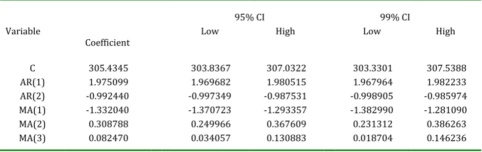
(4) Furthermore, it can be clearly seen from Table 3 that the coefficients are all significant as the p-values are less than α = 0.05 and confidence intervals at 90%, 95% and 99% is also

presented in Table 4.

Table 4. Confidence intervals of coefficients of ARIMA (2, 0, 3)

95% CI 99% CI

Variable

Coefficient Low High Low High

C 305.4345 303.8367 307.0322 303.3301 307.5388

AR(1) 1.975099 1.969682 1.980515 1.967964 1.982233

AR(2) -0.992440 -0.997349 -0.987531 -0.998905 -0.985974

MA(1) -1.332040 -1.370723 -1.293357 -1.382990 -1.281090

MA(2) 0.308788 0.249966 0.367609 0.231312 0.386263

MA(3) 0.082470 0.034057 0.130883 0.018704 0.146236

4.3.Diagnostic Checking

This is an examination of the goodness of fit of the selected model and it is usually on the basis of the residual analysis. The common diagnostic tools among others are Autocorrelation Function (ACF), Partial Autocorrelation Function (PACF) and Ljung-Box Q- Statistics (Q-Stat) of the residuals. The Ljung-Box Q- Statistics is considered as an overall check of goodness of fit of a model by testing presence of serial correlation in the residuals. For a given series of length , (NIST/SEMATECH, 2013) noted that the test statistic is defined as:

(5)

Where Estimated autocorrelation of the series at lag k Sample size (the number of residuals)

Number of lags being tested

Degrees of freedom

Number of parameters from the model fit to the data

This statistic will subject the residuals to the fulfilment of the models assumption of being independent and normally distributed based on the following hypotheses:

Ho: Residuals are random (white noise)

102

International Journal of Science and Business

Published By

Decision: If the value is less than critical value of at specified significance level, do not

reject the null hypotheses (Ho)

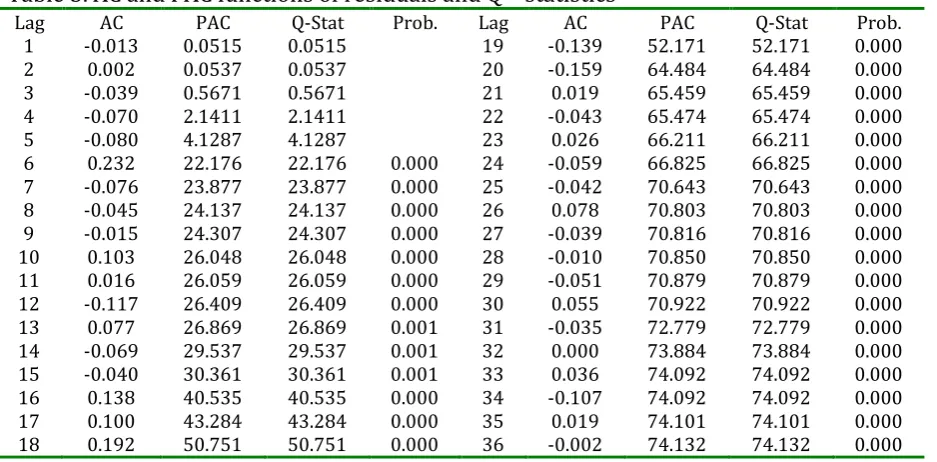
Table 5 presents the ACF, PACF and Q – Statistics at various lags and it can be observed that the values of the both ACF and the PACF revolve around zero meaning that the residuals are independent.

Table 5. AC and PAC functions of residuals and Q – statistics

Lag AC PAC Q-Stat Prob. Lag AC PAC Q-Stat Prob.

1 -0.013 0.0515 0.0515 19 -0.139 52.171 52.171 0.000

2 0.002 0.0537 0.0537 20 -0.159 64.484 64.484 0.000

3 -0.039 0.5671 0.5671 21 0.019 65.459 65.459 0.000

4 -0.070 2.1411 2.1411 22 -0.043 65.474 65.474 0.000

5 -0.080 4.1287 4.1287 23 0.026 66.211 66.211 0.000

6 0.232 22.176 22.176 0.000 24 -0.059 66.825 66.825 0.000

7 -0.076 23.877 23.877 0.000 25 -0.042 70.643 70.643 0.000

8 -0.045 24.137 24.137 0.000 26 0.078 70.803 70.803 0.000

9 -0.015 24.307 24.307 0.000 27 -0.039 70.816 70.816 0.000

10 0.103 26.048 26.048 0.000 28 -0.010 70.850 70.850 0.000

11 0.016 26.059 26.059 0.000 29 -0.051 70.879 70.879 0.000

12 -0.117 26.409 26.409 0.000 30 0.055 70.922 70.922 0.000

13 0.077 26.869 26.869 0.001 31 -0.035 72.779 72.779 0.000

14 -0.069 29.537 29.537 0.001 32 0.000 73.884 73.884 0.000

15 -0.040 30.361 30.361 0.001 33 0.036 74.092 74.092 0.000

16 0.138 40.535 40.535 0.000 34 -0.107 74.092 74.092 0.000

17 0.100 43.284 43.284 0.000 35 0.019 74.101 74.101 0.000

18 0.192 50.751 50.751 0.000 36 -0.002 74.132 74.132 0.000

To justify the goodness of fit of the chosen model , the reports of performance metric (Mean Absolute Percentage Error also MAPE) and histogram of the residuals of the model were examined. The in-sample computed value of this metric is and this indicated that error of forecast is within 10 percent error. Furthermore, the model yielded MAPE of 0.178 for out of sample forecast. Additionally, a good model is one where the coefficient of determination is less than Durbin Watson (DB) (Onasanya & Adeniji, 2013) and the values of these statistics based on are respectively 0.8478 and 2.002. It is clear that the R2 _{is lower than the DB confirming the goodness of fit of the .}

However, Ljung-Box Q-Statistics highlighted that the hypothesis that the Residuals are non-random is not rejected at 5% level of significance for lag 6 through lag 36.

Likewise, it can be deduced from Figure 5 that the residuals based on are normally distributed as the bars of the histogram shown symmetric pattern indicating the fitness of the selected model to the underlying process.

0 40 80 120 160 200

-10 -8 -6 -4 -2 0 2 4 6 8 10 12 14 16

F

re

q

u

e

n

c

y

Residuals

103

International Journal of Science and Business

Published By 5. Results and Discussions

The Naira – US Dollar Exchange Rates series is subjected to stationarity test by using three different approaches, namely: Augmented Dickey – Fuller (ADF) Test, runs sequence plot and Correlogram and in either case the series turned out stationary at level. On a quantitative note, this claim could be clearly seen from the fact that ADF Statistics presented in Table 1 are less than the test critical values at the significance levels of 1%, 5% and 10% with exceptional case at level without intercept and trend, meaning that the process is not a random walk. This result is further highlighted by the runs sequence plot (Figure 1) as it contains neither time variant trend nor seasonal cycles and a rapidly decayed Correlogram structure of the series at level as depicted in Figure 2. This finding is in agreement with the discovery that the Naira to Dollar assumes ARIMA (1,0,0) as opined by (Nwankwo, 2014). However, this discovery is contrary to the findings reported by (Onasanya & Adeniji, 2013), where the monthly Naira – US Dollar exchange rates series tends to be moving with time, which indicates that the parity series is non-stationary. Since the process is stationary at level, it can be concluded that the process could be best fit by ARMA (p, q). It can be observed that the parsimonious model is ARMA (2, 3) since it exhibited less BIC value of and the mathematical structure is given in equation (2). The model is unalike with models reported by (Nwankwo, 2014) and (Onasanya & Adeniji, 2013) because they respectively identified ARIMA (1,0,0) and ARIMA (1,2,1) as suitable models for forecasting the Naira – US Dollar exchange rate. This dissimilarity may be attributed to the policy shift, which is the basis of this research. An examination of the goodness of fit of the selected model based on performance metric (Mean Absolute Percentage Error) indicated that the error of forecast is within 10 percent. This implies that the model exhibit high accuracy and this claim is in line with the classification: MAPE values under 10% as high accuracy (Akincilar et al., 2011). The computed value of this metric is . The measure also correlated with the findings of (Tlegenova, 2015), who reported that the MAPE was 4.45 per cent for US dollar, 4.64 percent for euro, and 3.69 percent for Singapore dollar rates all against Kazakh tenge. Similarly, (Nwankwo, 2014) discovered that ARIMA(1,0,0) is suitable for forecasting the yearly Naira-US Dollar parity. He further stated that the residual is negligible based on the identified model. Additionally, (Abdullah, 2012) reported that ARIMA (2, 1, 2) turns out model with error of forecast less than 10 percent. He also noted that the measure indicates that the forecasting of gold bullion coin selling prices inaccuracy is low. Furthermore, the model yielded MAPE of 0.178 for out of sample forecast. Nevertheless, the residuals based on are normally distributed as the bars of the histogram (Figures 5) displayed symmetric pattern. However, Ljung-Box Q-Statistics highlighted that the hypothesis that the residuals are non-random is not rejected at 5% level of significance for lag 6 through lag 36 in line with the existence of serial correlation in the exchange rates series of interbank market as discovered by (Emenike, 2016). Further suitability of the selected model is evident from the fact that the coefficient of determination is less than Durbin Watson (DB). This finding is in line with opinion that a good model is one where the is less than DB (Onasanya & Adeniji, 2013) and the values of these statistics based on are respectively 0.8478 and 2.002.

6. Conclusion

104

International Journal of Science and Business

Published By

parity between the two currencies. However, the non-randomness of the residuals based on Ljung – Box test and the percentage of variations explained by the past rates and innovations on the basis of may be regarded as suggestion to consider other models than ARMA for modelling the Naira-US Dollar parity, hence the need for further investigation.

7. References

Abdalla, S. Z. S. (2012). Modelling Exchange Rate Volatility using GARCH Models : Empirical Evidence from Arab Countries. 4(3), 216–229. https://doi.org/10.5539/ijef.v4n3p216 Abdullah, L. (2012). ARIMA Model for Gold Bullion Coin Selling Prices Forecasting.

International Journal of Advances in Applied Sciences(IJAAS), 1(4), 153–158. Retrieved from

http://www.iaesjournal.com/ojs237/index.php/IJAAS/article/download/1495/755 Akincilar, A., TemIz, I., & ŞahIn, E. (2011). An application of exchange rate forecasting in

Turkey. Gazi University Journal of Science, 24(4), 817–828.

Appiah, S. T., & Adetunde, I. A. (2011). Forecasting Exchange rate between the Ghana Cedi and the US dollar using time series analysis. Current Research Journal of Economic Theory, 3(2), 76–83.

Brownlees, C. T., Engle, R. F., & Kelly, B. T. (2011). A Practical Guide to Volatility Forecasting through Calm and Storm. SSRN Electronic Journal, 14(2), 1–37. https://doi.org/10.2139/ssrn.1502915

Central Bank of Nigeria. (2016). Statistical Bulletin (Vol. 27).

Dimitrios, A., & Stephen, G. H. (2011). Applied Econometrics (Second Edi). Hampshire: PALGRAVE MACMILLAN.

Emenike, K. O. (2016). Comparative analysis of bureaux de change and official exchange rates volatility in Nigeria. Intellectual Economics, 000(1), 1–10. https://doi.org/10.1016/j.intele.2016.04.001

Indrabayu, N. H., Pallu, M. S., & Achmad, A. (2013). Statistic Approach versus Artificial Intelligence for Rainfall Prediction Based on Data Series. International Journal of Engineering and Technology (IJET), 5 No 2, 1962–1969.

Jianan Han, X.-P. Z., & Fang Wang. (2016). Gaussian Process Regression Stochastic Volatility Model for Financial Time Series. IEEE JOURNAL OF SELECTED TOPICS IN SIGNAL PROCESSING,10, NO. 6, 1015–1028.

Laessing, U., & Brock, J. (2016). Update 5-Nigeria to Abandon Naira Peg in Favour of Open Market Trading. Retrieved August 20, 2017, from Reuters website: http://www.reuters.com/news/archive/marketsNews

Mojekwu, J. N., Okpala, O. P., & Adeleke, I. A. (2011). Comparative analysis of modes of monetary exchange rates in Nigeria. 5(34), 13025–13029. https://doi.org/10.5897/AJBM11.2080

Nasiru, M. O., & Olanrewaju, S. O. (2015). Forecasting Airline Fatalities in the World Using a Univariate Time Series Model. 5(5), 223–230. https://doi.org/10.5923/j.statistics.20150505.06

NIST/SEMATECH. (2013). e-Handbook of Statistical Methods. Retrieved from http://www.itl.nist.gov/div898/handbook/

Nwankwo, S. C. (2014). Autoregressive Integrated Moving Average (ARIMA) Model for Exchange Rate (Naira to Dollar). Academic Journal of Interdisciplinary Studies, 3(4), 429– 434. https://doi.org/10.5901/ajis.2014.v3n4p429

105

International Journal of Science and Business

Published By

Dollar Using Time Domain Model. 1(1), 45–55.

Pankratz, A. (2009). Forecasting with univariate Box-Jenkins models : concepts and cases. New York: Wiley.

Sidehabi, S. W., Indrabayu, & Tandungan, S. (2016). Statistical and Machine Learning approach in forex prediction based on empirical data. 63–68. https://doi.org/10.1109/CyberneticsCom.2016.7892568

Sullivan, E. J. (2001). Exchange rate regimes: is the bipolar view correct? Journal of Economic Perspectives,15(2), 3–24.

Tlegenova, D. (2015). Forecasting Exchange Rates Using Time Series Analysis: The sample of the currency of Kazakhstan. 1–8.

Cite this article:

Maigana Alhaji Bakawu, Ahmed Abdulkadir, Shafiu Usman Maitoro & Abdulrahman Malik (2020). Evaluation of Models for Forecasting Daily Foreign Exchange Rates Between Nigerian Naira and US Dollar Amidst Volatility. International Journal of Science and Business, 4(1), 95-105. doi: 10.5281/zenodo.3601100

Retrieved from http://ijsab.com/wp-content/uploads/448.pdf