Admissibility of Linear Predictors of Finite Population
Parameters under Reflected Normal Loss Function
R. Jafaraghaie, and N. Nematollahi
*Department of Statistics, Faculty of Mathematical Sciences and Computer, Allameh Tabataba’i University, Tehran, Islamic Republic of Iran
Received: 2 August 2015 / Revised: 29 January 2016 / Accepted: 10 August 2016
Abstract
One of the most important prediction problems in finite population is the
prediction of a linear function of characteristic values of a finite population. In this
paper the admissibility of linear predictors of an arbitrary linear function of
characteristic values in a finite population under reflected normal loss function is
considered. Under the super-population model, we obtain the conditions for which
the linear predictors are admissible. Also, the risk of some admissible and
inadmissible predictors are compared by a simulation study.
Keywords: Admissibility; Finite population; Linear predictor; Reflected normal loss function; Super-population model.
*Corresponding author: Tel: +982144737546; Fax: +982144737547; Email: [email protected]
Introduction
A finite population is a collection of identifiable objects or elements. The students in a school, the households in a certain locality and etc. are examples of finite populations. A finite population of
N
units is denoted by index setU
{1,2,..., }
N
and the characteristic value associated withi
th unit in the population is denoted byy i
i, 1,2,..., .
N
The vector1
( ,... )
T Ny
y
y
is the unknown state of nature. Infinite population, we usually want to estimate a linear function of characteristic values such as total value
1 , N
i i
Y
y
mean value Y (
iN1y
i) /
N, or generally ( )y
iN1p y
i i,
where pi0, 1,...,i N
are known values. To estimate
( ),
y
we first choosea sample
s
{1,2,..., }
N
with associated characteristic valuesy
s
{ ,
y k s
k
}
by anarbitrary sampling design
p s
( )
(p s
(
)
0
, and ( ) 1s S
p
s
whereS
is any subset of{1,2,..., }
U
N
). Then, from this sample we estimate( )
y
by an estimator
( )
y
s.
The problem of estimation of an arbitrary linear function of the characteristic values
1 ( ) Ni
p y
i i,
y
in a finite population, has been considered and studied in the literature. One of the most interesting estimation problems is the admissibility of a given estimator. The problem of admissibility of an estimator of
( )
y
( )
p s
), Godambe [7] proved that the Horvitz-Thompson [12] estimator is admissible in the class of linear unbiased estimators under the Squared Error Loss (SEL) function. Godambe and Joshi [9] extended Godambe's [7] result and proved that the Horvitz-Thompson estimator is admissible in the class of all unbiased estimators. For more details, see Xu [26], He and Xu [11], Hu et al. [13] and Peng et al. [20]. Also, the problem of Bayes estimation of
( )
y
in finite population is considered in the literature by many researchers. For more details, see Joshi [14], Mashayekhi [18], Karunamuni and Zhang [15], Ghosh and Sinha [10], Bansal and Aggarwal [3], Chen et al. [6], Si et al. [22] and Zangeneh and Little [27].In model-based approach, the values
y
1,...,
y
N in a population are considered as a realization of random variablesY
1,...,
Y
N. The finite population may, therefore, be looked upon as a sample from a super-population. In this case, estimation of1
( ) Ni
p y
i i y
based on the sample
s
is knownas prediction of a function of unobserved y's. Bolfarine [2] considered the prediction of the total of characteristic values
( )
y
iN1y
i,
in a finitepopulation under the LINEX loss function. He obtained the Bayes estimators and discussed
the admissibility of these estimators. Zou [28] obtained all admissible linear estimators of
( )
y
under the LINEX loss function. Zou et al. [29] found all admissible linear estimators of
( )
y
in the class of linear and all estimators under the SEL function.In literature, the prediction of the unknown value
( )
y
is achieved only under SEL and LINEX loss functions. These loss functions are symmetric and asymmetric functions of
( )
y
s
( ),
y
respectively. But both of these losses are unbounded and are not appropriate for prediction of
( )
y
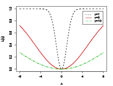
. As an alternative, Spiring [23] in response to this criticism, suggests the Reflected Normal Loss (RNL) function, which is defined by2 2 2
( )
(
1
)
,
L
k
e
(1)where
k
is the maximum loss and
is a shape parameter (see also Spring and Yeung [24]). The RNL function is a symmetric and bounded function of
,and is essentially a normal density flipped upside down, whence its name (Figure 1). Without loss of generality, we assume
k
1
.According to our best knowledge, in the literature, there is no trace of obtaining the admissible predictor of
( )
y
under the RNL function. So, in this paper we consider the problem of admissible prediction of( )
y
under the RNL function based on the super-population model.This article is organized as follows. In the next section, we give some definitions, notations and preliminary results which are used throughout the paper. In the main result section, we provide sufficient conditions for admissibility of linear predictors of
( )
y
under the RNL function using the super-population model with known variance. Besides, there are some results illustrated by simulation study in the application section. Finally, a discussion is given in discussion section.Preliminaries
In this section, we give some definitions and preliminary results which are used in the subsequent sections.
Finite population
In a finite population with index set
{1, 2,..., }
U
N
, the vector of characteristic values1
( ,... )
y
y
N T
y
is the unknown state of nature andis assumed to belong to
R
N. A subsets
of{1,2,..., }
N
is called a sample andn s
( )
denote the number of elements belonging tos
. We consider afixed number of sample, i.e.,
n s
( )
n
. A sample of sizen
is denoted byy
s
( ,..., )
y
i1y
in T
. In someprediction problems, it is necessary to predict a linear function of characteristic values of finite population. As in Zou et al. [29], we consider a general case, i.e., the prediction problem of an arbitrary linear function
1
(
)
Nkp
k ky
,
p
k0.
y
Super-population model
We consider the model-based or super-population approach in which
y
is viewed as arising from arandom sample of
N
units from some super-population having a probability density function (p.d.f) given byf yi
( | )
where
may be either known or some unknown super-population parameter (Pfeffermann and Rao [19]). The model-based approach considers the valuesy
1,...,
y
N in the population as a realization of random variables1
,...,
NY
Y
. The finite population may, therefore, be looked upon as a sample from a super-population distribution. After the sample has been observed, estimating
( )
y
reduces to predicting a function of unobservedY
's. In Bayesian point of view,
is a random variable with density function
( )
, which is known as prior distribution.Consider the following model for
y
, (2)(3)
where
k
1,2,...,
N
,
a
k
0 andb
k are known constants and
is unknown parameter. This model is a basic and very useful one in survey sampling and was discussed in detail by Cassel et al. [4,5]. Also, Godambe [8] and Zou [28] considered this model.Under the model (2) we assume
2 0
( , )
1,..,
~
,
k
N
k
N
. Hence, we have(4)
2 2
1 ( )
2 0 0 1,...,
1
( | ) , , , , . 2
k k k
y a b
k k N
f y e a k
Assuming a normal prior for
with p.d.f.(5) 2
0 2
0
1 ( )
2 0
1
( )
,
,
2
e
areknown
then the posterior p.d.f. of
giveny
s
is( , )
N
w
with0
2
2 2 2
2 2 2 2 2 2
( )
, ,
k k k
k s
s s s
a y b
and w
d d d
where
d
s
k sa
k2.
Posterior risk function of a predictor under RNL function using normal model
Following Towhidi and Behboodian [25], the posterior risk of a predictor
( )
y
s
under the RNL function using normal model is given by(6)
* 2 2
* 2
2 1
1 ( ( ) ( )) ( ( ) )
2( )
2
2 *
( , ( )) 1
(
s |)
1 w s ,s E e s e
w
y y y
y y
where
*
( ( ) | ),
*
( ( ) | ).
s s
E
and w
V
y y
y y
Hence, the posterior risk as a function of
is minimized when
( )
y
s
E
( ( ) | )
y y
s
*,
which is the same as Bayes predictor of
( )
y
under the SEL function. From (5), the posterior risk of( )
s
y
is2 *
( ( ), )) 1
.
w
(7)Since the posterior risk does not depend on
y
s,
therefore the Bayes risk of
( )
y
s is2 *
( , ( )) 1s .
r
w
y
å (8)
In the next section, we obtain the admissible linear predictors of
( )y
Nk1p
k ky . 0
2 2
0 0
,
( ) , ( ) , ( ) , ,
k k k k
k k k l
y a b
E E E k l
Results
In this section, we obtain the admissible predictor of
( )y
Nk1p
k ky under the RNL function,
using model (2) with normal assumption and known
2
. The main result is given in the following theorem.Theorem 1
Using super-population model (2) with normal assumption and known
2, under the RNL function, the predictorT s
( )
k sw y
ks k
w
0s with(
)
ks s k k
w
a
p k s
, of linear function
( )
y
is admissible in the class of all linear predictors, if one of the following two conditions is satisfied:( )
i
0
s
c d
s/
s, wherec
s
k sp a
k kand 2 s k k s d a
,( )
ii
s
c d
s/
s, and0s
(
s k s k k k s k k).
sc
w
a b
p b
d
Proof: Using the transformation
y
k
b
k
y
k, we need only to consider the caseb
k
0,
1,..., .
N
k
In this case, the condition( )
ii
becomes0 0
/
( )
ii
s
c d and w
s s s
.After some calculations, using model (2) and under the RNL function, the risk function of the predictor
0
( )
ks k sk s
T s
w y
w
of
( )
y
is given by(9) 2 2
2 2
1 ( ( ) ( ))
2( ) 2
2
( ( ), ( )) 1
(
T s)
1 m ,R T s E e e
m y y where
0 2 2 2
( ( ks k) k k k) s ( ( ks k) k).
k s k s k s k s
w p a p a w and m w p p
In order to prove the above theorem, we consider the following three cases.
(1) Assume
s
0. In this case0
( ) k s k k s
T s
p y w , and using (8) we have2 1 2 1 2( ) 2 1
( ( ), ( )) 1 m ,
R T s e
m y (10) where
0 2 2
1 s s 1 k. k s
w c and m p
Now assume
T s
( )
is not admissible and isdominated by the linear predictor
0
* *
ks k s
k sw y w
withw
*ks
s k*a
p
k . Using (8), we have2 2 2 2 2( ) 2 2
( ( ), ) 1 m ,
R e m
y (11) where 0* * 2 *2 2 2
2 s s s s 2 s s k. k s
d c w and m d p
Since
T s
( )
is dominated by
, we have( ( ), )
( ( ), ( )) ,
R
y
R
y
T s
which from (9) and (10) is equivalent to
2 2
2 1
2 2
2 1
2( ) 2( )
2 2
2 1
m m .
e e m m (12)
Let
w
0s/
c
s and therefore
1
0, so from (11) we have2 2 2 2 2( ) 2 2 2 1
m .
e m m (13)
Using the fact that
m
2
m
1, we have2 2
2 2
2 2
2 2
2( ) 2( )
2 2 2
2 1 1
m m .
e e
m m m
(14)
The inequality (13) contradicts the inequality (12), so the predictor
T s
( )
of
( )
y
is admissible for0
s
.(2) Assume 0
s
c d
s/
s. Let
have the prior distribution as in (4). The Bayes predictor of( )
y
(15)
2 2
0
2 2 2 2
( ) ( ( ) | ) ( s ) s .
s s k k k
k s s s
c c
E a p y
d d
y y y
Therefore when 0
s
c d
s/
s, the predictor0 0
( )
ks k s(
s k k)
k sk s k s
T s
w y
w
a
p y
w
is the Bayes predictor with respect to the prior distribution
N
( ,
0* 2*)
where0 0
2
* s
,
2* s.
s s s s s s
w
c
d
c
d
We can easily obtain the Bayes risk of
T s
( )
by using (7). After some calculations, we can show that the Bayes risk ofT s
( )
is finite. Now, since the loss function (1) is bowl-shaped, thenT s
( )
is the unique Bayes predictor and hence admissible.(3)When
s c d
s/
s andw
0s
0, by using the limiting Bayes method (see Blyth [1] and Lehmann and Casella [17]), we can show thatT s
( )
is admissible. In fact, from (9), the risk function of thepredictor ( )
(
s)
k k k k s
s
c
T s a p y
d
of
( )
y
is given by2 3
( ( ),
( ))
1
,
R
T s
m
r
y
(16) where2 2 2
3
(
( )
s s k)
.
s k s
c
m
d
p
d
Suppose that the predictor
T s
( )
is dominated by*
, then*
( ( ), )
( ( ), ( ))
,
R
y
R
y
T s
for all
(17)0 *
( ( ), )
( ( ), ( ))
.
R
y
R
y
T s
for some
(18)Since
R
( ( ), )
y
*
is a continuous function of
,then there exist an
0 and
1
2 such that *1 2
( ( ), ) ( ( ), ( )) .
R y R y T s for all
(19)
Let
B be the Bayes predictor with respect to the prior distributionN
( , )
0
B2 , and letr
*( )
B be theBayes risk of
B. From (14), we have2 2 2
( ) ( B s ) .
B s k k k
k s B s
c a p y
d
y (20)From (7), the Bayes risk of
B could be obtained as*
2 *
( ) 1B ,
B r w
(21) where 2 2* 2 2
2 B s2 .
B s k
k s B s
c
w d p
d
Let
r
* *( )
be the Bayes risk of the predictor
* with respect to the prior distributionN
( , ).
0
B2 Then from (15), (17), (18) and (20), we get2 2 2 1 2 2 2 1 1 2 * * * * 2 2 2
2 2 2
2 2 2
2 2 1 2 2 2 2 2 2 1 [ ( ( ), ( )) ( ( ), )] 2 ( ) ( ) 2 B B B B s B s s k s k
s k s k s B s B B s s k B s
R T s R e d
r r r r
c
c d p d p
d d
e d
c d p
d y y 2
2 2 2
2 2 s
s k s k s k s
c d p
d
when
B
.
Thus, if
B is sufficiently large, thenr
*( )
*
r
*( )
B , which contradicts the fact that
B is the Bayes predictor with respect to the prior distributionN
( , )
0
B2 . Therefore,T s
( )
is admissible. Cases (1)-(3) complete the proof of the Theorem.Remark 1
Following Lehmann [16] under the general loss function
L
( ( ), ( ))
y
y
s
, an estimator
( )
y
s isrisk unbiased estimator of
( )
y
if it satisfies (21)( ( ), ( ))s ( ( ), ( )) ,s ( ) ( ).
E L y y E L y y y y
unbiasedness, i.e.,
E
( ( ))
y
s
( )
y
, and if anestimator
( )
y
s
is notunbiased, then its bias is given by
( ( ))
s( ( ))
s( ).
Bias
y
E
y
y
So, the riskunbiased condition and bias of an estimator are depend on the loss function that we use. Under the RNL function, the risk unbiased condition (21) reduces to
2 2
1 ( ( ) ( )) 2
2
1 ( ( ) ( ))s s 0 .
E
e
y y
y y
Therefore we can define the risk bias of an estimator
( )
y
s
of
( )
y
under the RNL function as(22)2 2
1 ( ( ) ( )) 2
2 1
( ( ))s ( ( )s ( )) s .
Risk Bias E e
y y
y y y
In what follows, we use (22) to compute the risk bias of the given estimators in a simulation study.
Comparison of the predictors using simulation data In this section, we perform a simulation study to compare the predictors of Y (
Ni1yi ) /Nunder RNL function. For generating a population of size
N
1000
, we generate a random sample from normal distributions with different values of variance2 0.01, 0.1, 0.25, 0.5, 1
and meansa
k
,
1,...,1000
k
, where
3,4,5,7
and1 1000
( ,...,
)
a a
a
is an arbitrary vector of positiveelements. The population consist of these
N
1000
data. Now we extract samples of size
5,10,15, 20,50
n
and compute predictors, riskfunction and risk bias of them. Repeat this tasks
4
10
B
times and calculate the estimated risk function and risk bias of the predictors as a comparative tool. The simulation study proceeds as follows:1. Generate a sample with size 1000 from normal distributions:
N a
(
k
, ),
2k
1,...,1000
.2. Use simulation data as a population and extract samples of size
n
5,10,15, 20,50.3. Calculate the predictors for each sample as follows:
1 2 0
1 2
3
( ) ( ) , ( ) ( ) ,
2 4
( ) ( ) , ( ) (2 ) .
a s a s
s k k k s k k k s
s s
k s k s
n s n s
s k k k s k k k
s s
k s k s
c a p y c a p y w
d d
c a p y c a p y
d d
y y
y y
Where
1a and
2a are admissible predictors satisfying the conditions of Theorem 3.1 and the predictors
1nand
2n don’t satisfying those conditions. We setw
0s
c
s in
2a.4. Repeat steps 2-3
B
10
4 times and calculate the value of estimated risk function (ERF) and estimated absolute risk bias (EARB) of the predictors using the following formulas:2 2
1 1
1 B exp{ ( k ( )) / 2 }, i 1,2, , ,
ij j
ERF k a n
B
y
2 2 2
1
1 B ( ( ))exp{ ( ( )) / 2 }/ , 1,2, , ,
k k
ij ij
j
EARB i k a n
B
y y
where
2
and
ijk is the predictor,
1,2,
,
k
i
i
k a n
inj
th repetition ofsampling. Tables 1-5 present the estimated risk function and estimated risk bias (in parenthesis) of the predictors for different values for
and . From these tables we observe that
1a and
2a have the smallest risk among the four predictors and dominate1n
the estimated risk bias of admissible predictors
1a and
2a decreases and the estimated risk bias of inadmissible predictor
1n increases. The estimatedrisk bias of
2n for small values of
(
3,4)
decreases and for large values of
(
5,6)
increases as
2increases. Also, when
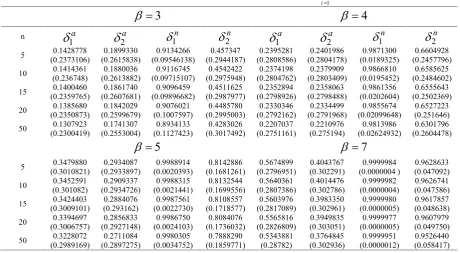
increases,Table 1.Simulated risk function and estimated risk bias (in parenthesis) for some predictors of 1 1
N i N
i
Y y
for20.01and different values of ß.3
4
n
1a
2a1n
2n1a
2a1n
2n5 (0.2378885)0.1428431 (0.2625259)0.1894101 (0.0944558)0.9148669 (0.2991968)0.4597269 (0.2813828)0.2396994 (0.2813643)0.2398510 (0.0185136)0.9874875 (0.247265)0.6652028
10 (0.2370966)0.1415236 (0.2618272)0.1877090 (0.09632349)0.9127647 (0.2998343)0.4563263 (0.2807716)0.2376270 (0.2807872)0.2377781 (0.01923796)0.9869354 (0.2488868)0.6616230
15 (0.2362677)0.1401947 (0.2610655)0.1859913 (0.09820985)0.9106133 (0.3002461)0.4530182 (0.280125)0.2355348 (0.2801496)0.2356786 (0.01998987)0.9863571 (0.2503771)0.6579932
20 (0.2354049)0.1388338 (0.2602587)0.1842195 (0.1000972)0.9084416 (0.3005806)0.4498847 (0.2794499)0.2334017 (0.2794721)0.2335183 (0.02076099)0.985760 (0.2517787)0.6544659
50 (0.2302795)0.1310484 (0.2554332)0.1741602 (0.1120913)0.8942346 (0.302154)0.4296163 (0.2752824)0.2210316 (0.2753181)0.2211499 (0.02600919)0.9815972 (0.2602871)0.6315701
5
7
5 (0.3014971)0.3483347 (0.2943094)0.2932344 (0.0019661)0.9989370 (0.1670604)0.8190645 (0.279817)0.5680374 (0.3030775)0.4045212 (0.0000003)0.9999985 (0.0453183)0.9649467
10 0.3455610(0.301297) (0.2939112)0.2908026 (0.0020930)0.998863 (0.169103)0.8161054 (0.2807682)0.5644279 0.4014696(0.30317) (0.0000004)0.9999983 (0.0465601)0.9638405
15 (0.3010653)0.3427571 (0.2934564)0.2883346 (0.0022284)0.9987834 (0.1711256)0.8130285 (0.2817032)0.5607679 (0.3032171)0.3983638 (0.0000004)0.9999981 (0.0478674)0.9626497
20 (0.3008114)0.3399043 (0.2929672)0.2857999 (0.0023712)0.9986990 (0.173091)0.8099853 (0.2826323)0.5570451 (0.3032416)0.3951813 (0.0000005)0.9999978 (0.0491847)0.9614380
50 (0.2990046)0.3231801 (0.2898401)0.2711817 (0.0034317)0.9980577 (0.1854963)0.7899758 (0.2877669)0.5347707 (0.3030189)0.3765925 0.9999952(.0000011) (0.0580150)0.9530882
Table 2.Simulated risk function and estimated risk bias (in parenthesis) for some predictors of 1 1
N i N
i
Y y
for20.1and different values of ß.3
4
n
1a
2a
1n
2n
1a
2a
1n
2n 5 (0.2373106)0.1428778 (0.2615838)0.1899330 (0.09546138)0.9134266 (0.2944187)0.457347 (0.2808586)0.2395281 (0.2804178)0.2401986 (0.0189325)0.9871300 (0.2457796)0.660492810 (0.236748)0.1414361 (0.2613882)0.1880036 (0.09715107)0.9116745 (0.2975948)0.4542422 (0.2804762)0.2374198 (0.2803409)0.2379909 (0.0195452)0.9866810 (0.2484602)0.6585625
15 (0.2359765)0.1400460 (0.2607681)0.1861740 (0.09896682)0.9096459 (0.2987977)0.4511625 (0.2798926)0.2352894 (0.2798488)0.2358063 (0.0202604)0.9861356 (0.2502369)0.6555643
20 (0.2350873)0.1385680 (0.2599679)0.1842029 (0.1007597)0.9076021 (0.2995003)0.4485780 (0.2792162)0.2330346 (0.2791968)0.2334499 (0.02099648)0.9855674 (0.251646)0.6527223
50 (0.2300419)0.1307923 (0.2553004)0.1741307 (0.1127423)0.8934133 (0.3017492)0.4283026 (0.2751161)0.2207037 (0.275194)0.2210976 (0.02624932)0.9813986 (0.2604478)0.6301796
5
7
5 (0.3010821)0.3479880 (0.2933897)0.2934087 (0.0020393)0.9988914 (0.1681261)0.8142886 (0.2796951)0.5674899 (0.302291)0.4043767 (0.0000004 )0.9999984 (0.047092)0.9628633
10 (0.301082)0.3452591 (0.2934726)0.2909337 (0.0021441)0.9988315 (0.1699556)0.8132544 (0.2807386)0.5640361 (0.302786)0.4014476 (0.0000004)0.9999982 (0.047586)0.9626741
15 (0.3009101)0.3424403 (0.293162)0.2884076 (0.0022730)0.9987561 (0.1718577)0.8108557 (0.2817089)0.5603976 (0.302961)0.3983350 (0.0000005)0.9999980 (0.048638)0.9617857
20 (0.3006757)0.3394697 (0.2927148)0.2856833 (0.0024103)0.9986750 (0.1736032)0.8084076 (0.2826809)0.5565816 (0.303051)0.3949835 (0.0000005)0.9999977 (0.049750)0.9607979
the estimated risk of
1a (
1n and
2n) increases (decreases) and the estimated risk bias of
2a first increases and then decreases. Note that when thesample size
n
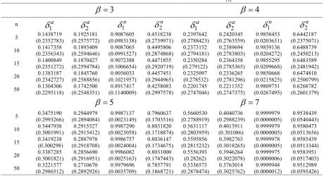
increases, the risk bias of all predictors increases, this phenomenon can be occurred in survey sampling as explained by Roxy et al. (2008, p. 34).Table 3.Simulated risk function and estimated risk bias (in parenthesis) for some predictors of 1 1
N i N
i
Y y
for20.25and different values of ß.3
4
n
1a
2a1n
2n1a
2a1n
2n5 (0.2365118)0.1431960 (0.260062)0.1908865 (0.0966448)0.9115639 (0.2865557)0.4547678 (0.2800806)0.2395511 (0.2788779)0.2408678 (0.0194958)0.9866324 (0.242833)0.6538721
10 (0.236301)0.1415035 (0.2606631)0.1885034 (0.0980132)0.9104396 (0.2937791)0.4521434 (0.2800624)0.2373271 (0.2796023)0.2383555 (0.0199069)0.9863708 (0.2472884)0.6546179
15 (0.2356288)0.1400149 (0.2602816)0.1864962 (0.0997134)0.9086203 (0.2962802)0.4493682 (0.2795864)0.2351373 (0.2793543)0.2360383 (0.0205573)0.9858843 (0.2495729)0.6526026
20 (0.2347427)0.1384136 (0.2595478)0.1843136 (0.1013973)0.9067399 (0.2976293)0.4473081 (0.2789364)0.2327655 (0.278786)0.2334847 (0.0212460)0.9853569 (0.2511275)0.6505791
50 (0.2298087)0.1306059 (0.2551177)0.1741591 (0.1133211)0.8926575 (0.3010142)0.4271461 (0.2749404)0.2204447 (0.2750165)0.2210941 (0.0264738)0.9812093 (0.2603998)0.6287511
5
7
5 (0.300417)0.3477413 (0.2918832)0.2937951 (0.0021444)0.9988243 (0.1692659)0.8071225 (0.2794111)0.5668848 (0.3009846)0.4042373 (0.0000004)0.9999982 (0.0498086)0.9594932
10 (0.3007459)0.3450271 (0.2927455)0.2911629 (0.0022086)0.9987910 (0.1708404)0.8092747 (0.2806239)0.5636358 (0.302147)0.4014227 (0.0000004)0.9999981 (0.0490660)0.9609117
15 (0.3006754)0.3421882 (0.292676)0.2885495 (0.0023251)0.9987235 (0.1725871)0.8079684 (0.2816531)0.5600385 (0.3025351)0.3983081 (0.0000005)0.9999979 (0.0497022)0.9605356
20 (0.3004834)0.3391139 (0.2923254)0.2856449 (0.0024543)0.9986474 (0.1741154)0.8062981 (0.2826762)0.5561552 (0.3027352)0.3948152 (0.0000005)0.9999977 (0.0505331)0.9598706
50 (0.2988092)0.3224979 (0.2895601)0.2710743 (0.0035174)0.9980038 (0.1863958)0.7875509 (0.2878439)0.5340508 (0.3028006)0.3763964 (0.0000012)0.9999950 (0.0588828)0.9520992
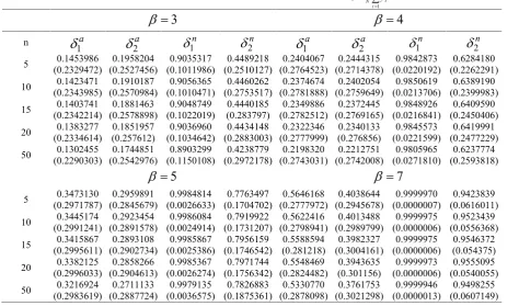
Table 4.Simulated risk function and estimated risk bias (in parenthesis) for some predictors of 1 1
N i N
i
Y y
for20.5and different values of ß.3
4
n
1a
2a
1n
2n
1a
2a
1n
2n 5 (0.2352783)0.1438719 (0.2575772)0.1925181 (0.0983138)0.9087605 (0.2739971)0.4518238 (0.2788423)0.2397642 (0.2763559)0.2420345 (0.0203631)0.9858453 (0.2375071)0.644218710 (0.2356343)0.1417358 (0.2594646)0.1893409 (0.0991527)0.9087065 (0.2874868)0.4495806 (0.2794181)0.2373152 (0.2783803)0.2389694 (0.0204272)0.9859136 (0.2450213)0.6488739
15 (0.2351272)0.1400849 (0.2594784)0.1870427 (0.1006654)0.9072388 (0.2920719)0.4471855 (0.279122)0.2350284 (0.2785365)0.2364358 (0.0209668)0.9855295 (0.2481942)0.6483589
20 (0.2342727)0.1383187 (0.2588856)0.1845760 (0.1021957)0.9056033 (0.2944965)0.4457451 0.2325097(0.278532) (0.2781296)0.2336265 (0.0215825)0.9850668 (0.2500799)0.6474810
50 (0.2295118)0.1304306 (0.2548351)0.1742500 (0.1140009)0.8917417 (0.2997578)0.4258083 (0.2747046)0.2201745 (0.2747375)0.2211352 (0.0267495)0.9809731 (0.2601379)0.6268782
5
7
5 (0.2993266)0.3475190 (0.2894084)0.2944979 (0.0023149)0.9987137 (0.1703516)0.7960637 (0.2788919)0.5660530 (0.2988239)0.4040736 (0.0000005)0.9999979 (0.0540443)0.9538439
10 (0.3001991)0.3447938 (0.2915412)0.2915527 (0.0023058)0.9987290 (0.1718874)0.8031820 (0.2803959)0.5631117 (0.301086)0.4013911 (0.0000005)0.9999979 (0.0513656)0.9580473
15 0.3419238(0.300298) (0.2918708)0.2887978 (0.0024004)0.9986757 (0.1734675)0.8036147 (0.2815232)0.5595856 (0.3018265)0.3982763 (0.0000005)0.9999978 (0.0513344)0.9585439
20 (0.3001821)0.3387285 (0.2916951)0.2856690 (0.0025163)0.9986082 (0.1747443)0.8031000 0.5556393(0.28262) (0.3022078)0.3946264 (0.0000006)0.9999975 (0.0517403)0.9583951
Discussion
In this paper we obtain sufficient condition of admissibility of linear predictors of
1 ( ) Nk p yk k
y
in the class of all linear
predictors under the RNL function. So, we could find admissible linear predictors of the total value
1
N
i i
Y
y and the mean value Y (
iN1yi) /Nof a finite population. Further research is needed to find the necessity condition of admissibility of linear predictors of
( )
y
under the RNL function. Weperform a simulation study to compare the predictors of Y (
iN1yi) /N that satisfy and do not satisfy the conditions of Theorem 3.1 under the RNL function. From Tables 1-5, for simulated data we observe that
1a and
2a have the smallest risks among the four predictors being considered and dominate
1n and
2n for all values of
and . So,
1n and
2n are inadmissible.Acknowledgments
The authors are grateful to referees for making helpful comments and suggestions on an earlier version of this paper which resulted in this improved version.
References
1. Blyth C. R. On minimax statistical decision procedures and their admissibility. Ann. Math. Statist., 22: 22-42 (1951).
2. Bolfarine H. A note on finite population prediction under asymmetric loss functions. Comm. Statist. Theory Methods,18: 1863-1869 (1989).
3. Bansal A. K. and Aggarwal A. K. Bayes prediction of the regression coefficient in a finite population using balanced loss function.Metron, 67(1):1-16 (2009).
4. Cassel C. M., sarndal C. E. and Wretman J. H. Some results on generalized difference estimation and generalized regression estimation for finite populations.
Biometrika,63: 615 -620 (1976).
5. Cassel C. M., Sarndal C. E. and Wretman J. H.
Foundations I71" Inference in Survey Sampling. Wiley, New York (1977).
6. Chen, Q., Elliott, M. R. and Little, R. J. A. Bayesian inference for finite population quantiles from unequal probability samples. Surv. Methodol., 38(2): 203-214 (2012).
Table 5.Simulated risk function and estimated risk bias (in parenthesis) for some predictors of 1
1
N i N
i
Y y
for
2 1
and different values of ß.
3
4
n
1a
2a
1n
2n
1a
2a
1n
2n5 (0.2329472)0.1453986 (0.2527456)0.1958204 (0.1011986)0.9035317 (0.2510127)0.4489218 (0.2764523)0.2404067 (0.2714378)0.2444315 (0.0220192)0.9842873 (0.2262291)0.6284180
10 (0.2343985)0.1423471 (0.2570984)0.1910187 (0.1010471)0.9056365 (0.2753517)0.4460262 (0.2781888)0.2374674 (0.2759649)0.2402054 (0.0213706)0.9850619 (0.2399983)0.6389190
15 (0.2342214)0.1403741 (0.2578898)0.1881463 (0.1022019)0.9048749 (0.283797)0.4440185 (0.2782512)0.2349886 (0.2769165)0.2372445 (0.0216841)0.9848926 (0.2450406)0.6409590
20 (0.2334614)0.1383277 (0.257612)0.1851957 (0.1034642)0.9036960 (0.2883003)0.4434148 (0.2777999)0.2322346 (0.276856)0.2340133 (0.0221599)0.9845573 (0.2477229)0.6419991
50 (0.2290303)0.1302455 (0.2542976)0.1744851 (0.1150108)0.8903299 (0.2972178)0.4238779 (0.2743031)0.2198320 (0.2742008)0.2212751 (0.0271810)0.9805965 (0.2593818)0.6237774
5
7
5 (0.2971787)0.3473130 (0.2845679)0.2959891 (0.0026633)0.9984814 (0.1704702)0.7763497 (0.2777972)0.5646168 (0.2945678)0.4038644 (0.0000007)0.9999970 (0.0616011)0.9423839
10 (0.2991241)0.3445174 (0.2891578)0.2923454 (0.0024914)0.9986084 (0.1731207)0.7919922 (0.2798941)0.5622416 (0.2989799)0.4013488 (0.0000006)0.9999975 (0.0556368)0.9523439
15 (0.2995611)0.3415867 (0.2902734)0.2893108 (0.0025386)0.9985867 (0.1746542)0.7956159 (0.281218)0.5588594 (0.3004161)0.3982327 (0.0000006)0.9999975 (0.054375)0.9546372
20 (0.2996033)0.3382125 (0.2904613)0.2858266 (0.0026274)0.9985367 (0.1756342)0.7971744 (0.2824482)0.5548469 (0.301156)0.3943635 (0.0000006)0.9999973 (0.0540055)0.9555095
7. Godambe, V. P. An optimum property of regular maximum likelihood estimation. Ann. Math. Statist., 4: 1208-1211 (1960).
8. Godambe V. P. Estimation in survey sampling: robustness and optimality. J. Amer. Statist. Assoc., 77: 393-406 (1982).
9. Godambe V. P. and Joshi V. M. Admissibility of Bayes estimation in sampling finite populations (I). Ann. Math. Statist.,36(6): 1707-1722 (1965).
10. Ghosh M. and Sinha K. Empirical Bayes estimation in finite population sampling under functional measurement error models.J. Statist. Plann. Inference, 137(9): 2759-2773 (2007).
11. He D. and Xu X. Admissibility of linear predictors in the superpopulation model with respect to inequality constraints under matrix loss function. Comm. Statist.
Theory Methods,40(21): 3789-3799 (2011).
12. Horvitz D. G. and Thompson D. G. A generalization of sampling without replacement from a finite universe. J. Amer. Statist. Assoc.,47: 663-686 (1952).
13. Hu G., Li Q. and Yu S. Optimal and minimax prediction in multivariate normal populations under a balanced loss function.J. Multivariate Anal.,128: 154-164 (2014). 14. Joshi V. M. A note on admissible sampling designs for a
finite population, Ann. Math. Statist., 42(4): 1425-1428 (1971).
15. Karunamuni R. J. and Zhang S. Optimal linear Bayes and empirical Bayes estimation and prediction of the finite population mean.J. Statist. Plann. Inference,113(2): 505-525 (2003).
16. Lehmann E.L. A general concept of unbiasedness. Ann. Math. Statist.,22: 578-592 (1951).
17. Lehmann E. L. and Casella G. Theory of Point Estimation. Springer Verlag, New York (1998).
18. Mashayekhi M. A note on linear empirical Bayes estimation of finite population means.J. Statist. Plann.
Inference,112(1): 77-88 (2003).
19. Pefeffermann D. and Rao C. R.Handbook of Statistics,6.
Elsevier Science, Amsterdam(2009).
20. Peng P., Hu G. and Liang J. All admissible linear predictors in the finite populations with respect to inequality constraints under a balanced loss function.J. Multivariate Anal.,140:113-122 (2015).
21. Roxy P., Chris O. and Jay D. Introduction to Statistics and Data Analysis, 3rd Edition, Brooks/Cole Cengage Learning (2008).
22. Si Y., Pillai N. and Gelman A. Bayesian nonparametric weighted sampling inference.Bayesian Anal.,10(3): 605-625 (2015).
23. Spiring F. A. The reflected normal loss function. Canad. J. Statist.,21(1): 321-330 (1993).
24. Spiring F. A. and Yeung A. S. A general class of loss functions with industrial applications. J. Qual. Technol.,
30: 152-162 (1998).
25. Towhidi M. and Behboodian J. Estimation of a location parameter with a reflected normal loss function. Iran. J. Sci. Technol. Trans. A Sci.,25(A1): 183-190 (2001). 26. Xu L. Admissible linear predictors in the superpopulation
model with respect to inequality constraints.Comm. Statist.Theory Methods,38(15):2528-2540 (2009). 27. Zangeneh S. Z. and Little R. J. A. Bayesian inference for
the finite population total from a heteroscedastic probability proportional to size sample. J. Surv. Statist. Methodo.,3(2): 162-192 (2015).
28. Zou G. H. Admissible estimation for finite population under the Linex loss function,J. Statist. Plann. Inference,
61: 373-384 (1997).