217 International Journal of Transportation Engineering, Vol.6/ No.3/ (23) Winter 2019
Modelling and Solving the Capacitated Location-Routing
Problem with Simultaneous Pickup and Delivery Demands
Ali Nadizadeh 1, Hasan Hosseini Nasab 2
Received: 19. 11. 2017 Accepted: 03.04.2018
Abstract
In this work, the capacitated location-routing problem with simultaneous pickup and delivery (CLRP-SPD) is considered. This problem is a more realistic case of the capacitated location-routing problem (CLRP) and belongs to the reverse logistics of the supply chain. The problem has many real-life applications of which some have been addressed in the literature such as management of liquid petroleum gas tanks, laundry service of hotels and drink distribution. The CLRP-SPD is composed of two well-known problems; facility location problem and vehicle routing problem. In CLRP-SPD, a set of customers with given delivery and pickup demands should be supplied by a fleet of vehicles that start and end their tours at a single depot. Moreover, the depots and vehicles have a predefined capacity and the objective function is minimizing the route distances, fixed costs of establishing the depot(s) and employing the vehicles. The node-based MIP formulation of the CLRP-SPD is proposed based on the literature of the problem. To solve the model, a greedy clustering method (GCM) is developed which includes four phases; clustering the customers, establishing the proper depot(s), assigning the clusters to depot(s) and constructing the vehicle tours by ant colony system (ACS). The numerical experiments on two sets of test problems with different sizes on the number of customers and candidate depots show the efficiency of the heuristic method with the proposed method in the literature. Finally, performance of the heuristic method to the similar methods in the literature is evaluated by several standard test problems of the CLRP.
Keywords: Capacitated location-routing problem; simultaneous pickup and delivery; greedy clustering method; ant colony system.
Corresponding author E-mail: [email protected] 1Assistant Professor, Department of
Industrial Engineering, Faculty of Engineering, Ardakan University, Ardakan, Iran
International Journal of Transportation Engineering, 218 Vol.6/ No.3/ (23) Winter 2019
1. Introduction and Literature
Review
In each supply chain, making the good strategies and decisions to reduce the logistic costs is the one of the important issues that should be considered more. In recent years, the efficient, reliable, and flexible decisions on location of depots and the vehicle routs are of vital importance for managers [Zare Mehrjerdi and Nadizadeh, 2013; Tavakkoli-Moghaddam et al.2016]. Logistic cost is usually related to the locating the distributing centers (DC) or depots and routing between the customers and depots by a fleet of vehicles [Zare Mehrjerdi and Nadizadeh, 2016]. Many researchers indicated that if the routes are ignored while locating the depots, the costs of distribution systems might be immoderate [Webb, 1968; Salhi and Rand, 1989; Prins et al.2006]. The location-routing problem (LRP) overcomes this drawback by simultaneously considering the location and routing decisions [Nadizadeh and Kafash, 2017].
The LRP is defined as a special case of vehicle routing problem (VRP) in which there is a need to solve the facility location problem (FLP), simultaneously [Zarandi et al.2011]. Since both problems belong to the class of NP-hard problem, the LRP is also NP-hard problem [Barreto et al.2007; Belenguer et al.2011]. LRP is applicable for a wide variety of fields such as food and drink distribution, newspapers delivery, waste collection, bill delivery, military applications, used oil management, organization of natural disaster, battery swap stations, parcel delivery and various consumer goods distribution [Manzour-al-Ajdad et al.2012; Rath and Gutjahr, 2014; Zhao and Verter, 2014; Yang and Sun, 2015].
In LRP, the customers should only be supplied by a single vehicle; in the other word the vehicle meets every customer once. Each vehicle also starts and ends its tour at a single depot. In the LRP, the proper depot(s) between candidate depots as well as the vehicle tours should be established. The objective is to minimize the total distance of routes as well as fixed depot and vehicle costs [Nadizadeh et
al.2011; Escobar, 2014]. Furthermore, the capacitated location-routing problem (CLRP) is a version of LRP that constrained by the vehicles and depots capacities [Nadizadeh and Nasab, 2014].
Laporte is the first researcher who discusses and classifies the LRP models [Laporte, 1988]. Min et al. [Min et al.1998] also review the LRP literature using a hierarchical classification based on the problem characteristics such as the number of depots, the capacity of depots and vehicles, the form of the objective function and etc. More recently, Nagy and Salhi [Nagy and Salhi, 2007] perform a comprehensive literature review on the LRP models, solution approaches, application areas and some future works. Since the solution times increase exponentially with an increase in the size of the problem, most papers in field of LRP and CLRP have focused on only new solution approaches that are often based on heuristic or meta-heuristic approaches [Nadizadeh et al.2017]. Some reviews on solution approaches of CLRP exist in literature that can be found in [Duhamel et al.2010; Derbel et al.2012; Zarandi et al.2013].
Recently, two review researches are carried out to survey recent publications of LRP’s Models; Prodhon and Prins analyzed the literature on the standard LRP and the extensions such as several distribution echelons, multiple objectives or uncertain data [Prodhon and Prins, 2014]. They also compared the results of state-of-the-art meta-heuristics on standard sets of instances for the classical LRP, the two-echelon LRP and the truck and trailer problem. Drexl and Schneider presented paper discussed variants and extensions of the standard LRP, which include problems with stochastic and fuzzy data, multi-period planning horizons, continuous location in the plane, multiple objectives, more complex demands or route structures, such as pickup and delivery demands or routes with load transfers, and inventory decisions [Drexl and Schneider, 2015].
Ali Nadizadeh, Hasan Hosseini Nasab
219 International Journal of Transportation Engineering, Vol.6/ No.3/ (23) Winter 2019
Table 1. Related works of the LRP-SPD
Author(s) Year Contributions and/or approaches.
[Karaoglan et al.2011] 2011 Branch-and-cut algorithm
[Karaoglan et al. 2012] 2012 Simulated anealing
[Yu and Lin, 2014] 2014 Multi-start simulated annealing
[Huang, 2015] 2015 LRP with pickup–delivery routes and stochastic demands + Tabu search
[Rahmani et al.2015] 2015 Two-Echelon Multi-products LRP-SPD + Local Search approach
[Yu and Lin, 2016] 2015 Simulated annealing
[Rahmani et al.2016] 2016 Two-Echelon Multi-products LRP-SPD + Nearest neighbour and
insertion approaches [Ghatreh Samani and
Hosseini-Motlagh, 2017] 2017 Two-Echelon LRP-SPD with fuzzy demands + Hybrid of SA and GA
[Wang and Li, 2017] 2017 LRP-SPD with heterogeneous fleet and time windows + Hybrid heuristic
algorithm (genetic algorithm + variable neighborhood algorithm)
only required to deliver goods to customers but also to pick up some goods from the customers, simultaneously. The CLRP-SPD arises in context of reverse logistics and there are various real cases, such as distribution of bottled drinks, chemicals, LPG (liquid petroleum gas) tanks, laundry service of hotels and etc. where the customers are typically visited for a double service. In the case of the bottled drinks for instance, full bottles are delivered to customers and empty ones are brought back either for reuse or for recycling [Nadizadeh, 2017]. In the CLRP-SPD, the problem is more complicated than CLRP because of the fluctuating loads on the vehicle along a route. In the CLRP, the total load of each route must not exceed the capacity of the vehicle. But in CLRP-SPD, the net change (decrease or increase) on the vehicle load at each customer must be monitored by the vehicle capacity [Catay, 2010]. As a result, the CLRP-SPD can reduce to a CLRP after some changes [Karaoglan et al.2012]. Because the CLRP is hard, the CLRP-SPD is also NP-hard.
LRP-SPD, a branch of LRP, was firstly introduced by Karaoglan et al. [Karaoglan et al.2011]. Although the LRP has been studied extensively in the literature, the LRP-SPD has received very little attention from researchers so far. Table 1 summarizes the related works on LRP-SPD, describing their main contributions and/or approaches. Karaoglan et al. [Karaoglan et al.2011] presented a mathematical
formulation for the CLRP-SPD and proposed an effective branch-and-cut algorithm for solving it. Their algorithm composed of several valid inequalities and a local search based on simulated annealing (SA) to obtain upper bounds. Finally to evaluate the proposed algorithm, they solved a large number of benchmark instances, derived from the literature, in a reasonable computation time. In next work, Karaoglan et al. [Karaoglan et al.2012] suggested two polynomial-size mixed integer linear programming formulations for the CLRP-SPD and a number of valid inequalities to strengthen the formulations. While their first formulation was a node-based formulation, the second one was a flow-based formulation. Furthermore, they proposed a two-phase heuristic approach based on SA, to solve the CLRP-SPD. They also generated the initial solutions by two initialization heuristics. Consequently, computational results showed that the flow-based formulation performs better than the node-based formulation in terms of the solution quality and the computation time on small-size problems.
International Journal of Transportation Engineering, 220 Vol.6/ No.3/ (23) Winter 2019
significantly enhance the performance of traditional single-start simulated annealing algorithm. Wang and Li [Wang and Li, 2017] studied on a low carbon for LRP with heterogeneous fleet, simultaneous pickup-delivery and time windows. They designed a two-phased hybrid heuristic algorithm to solve the problem. Firstly, the concept of temporal-spatial distance with genetic algorithm is used to cluster the customer points to construct the initial path. Then, variable neighborhood search algorithm is applied for local search. Computational results showed that the initial solution considering temporal-spatial distance has obvious advantages in the efficiency of the algorithm and the quality of the solution.
So far, many heuristic approaches have expanded in the literature of the LRP, which can be categorized in four main groups namely, sequential, clustering, iterative, and hierarchical methods. In sequential methods, in first step, the summation of depot to customer distances is minimized and then, the VRP is solved based upon the location of depots. The clustering-based methods, first create clusters for the customers, then, either solve the VRP for each candidate depot, or solve the traveling salesman problem (TSP) to find the best location of depots. In iterative heuristics, VRP and FLP sub-problems are solved iteratively, feeding information from one phase to the other. In hierarchical method, location of depots is the main problem and routing is a subordinate problem [Nagy and Salhi, 2007]. This paper presents a new efficient solution approach that belongs to clustering-based methods, based on the above classification. In fact, a greedy clustering method (GCM) is proposed to solve the CLRP-SPD in four phases. Since a greedy search algorithm is used for clustering the customers in first phase, the proposed method is called “greedy clustering method”. In second phase, among a set of candidate depots, the most appropriate one(s) are selected to be established. The third phase allocates the clusters to depot(s), and finally, ant colony system (ACS) is applied to set up the best routes between the depot(s) and the assigned clusters in fourth phase.
The remainder of this paper is organized as follows; In Section 2, problem definition with an example of CLRP-SPD including the mathematical formulation is given. Details of the proposed method are presented in section 3. In section 4, the computational results of numerical experiments are reported. Finally, conclusion and future directions of the paper are presented in section 5.
2.
Problem
Definition
and
Formulation
There are three entities in the CLRP-SPD that linked together. First, a number of candidate depots which have limited capacities. Second, some of the customers who have specific demands where consist of two parts: the receiving including shipping goods from / to the depot by a vehicle. Third, unrestricted number of fleet of homogeneous vehicles which have a predefined capacity should serve the customers. In the CLRP-SPD, each vehicle is used only in one route and starts and finishes its route at the same depot. Moreover, the total vehicle load at any point of the route should not exceed the vehicle capacity. On the other hand, each customer is served by exactly one vehicle and the total pickup and delivery load of the customers assigned to a depot should not exceed the capacity of the depot. The problem is to determine the locations of depot(s), the assignment of customers to the opened depot(s) and tour of vehicles with a minimum total cost [Karaoglan et al.2012].
Ali Nadizadeh, Hasan Hosseini Nasab
221 International Journal of Transportation Engineering, Vol.6/ No.3/ (23) Winter 2019
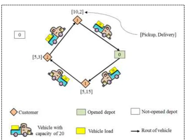
Figure 1. Illustrative example for the CLRP-SPD.
The node-based Mixed Integer Programming (MIP) formulation for the CLRP-SPD is proposed as follow. The formulation is adapted to Karaoglan et al. [Karaoglan et al.2012] with small changes. Let G = (N,A) be a complete directed network where N = N0 ∩ NC is a set of nodes in which N0 and NC represent the potential depot nodes and customers, respectively, and A = {(i, j): i, j∈N} is the set of arcs. Each arc (i, j) has a nonnegative cost (distance) cij that is based on Euclidian distance and triangular inequality holds (i.e., cij + cjk ≥
cik). A capacity Wk and a fixed cost Fk are associated with each potential depot k ∈ N0. Moreover, a capacity Q and fixed operating cost f are linked with an unlimited fleet of homogeneous vehicles. Each customer i∈ NC has pickup (pi) and delivery (di) demands, so that 0 ≤ di, pi ≤ Q. The variables used in the formulation of CLRP-SPD are given as follows:
Decision variables:
xij= {
1
0
if a vehicle goes directly from customer i to customer j (∀i,j∈N) otherwise
yk = {1
0
if depot k is opend (∀k∈N0)
otherwise
zik = {1
0
if customer i is assigned to depot k (∀i∈NC, ∀k∈N0) otherwise
Additional variables:
Ui : delivery load on vehicle just before serving customer i (∀i∈NC)
Vi : pickup load on vehicle just after serving customer i (∀i∈NC)
The node-based MIP formulation of the CLRP-SPD is given as follows:
Minimize ∑Fkyk+
k∈N0
∑ ∑cijxij+
j∈N i∈N
∑ ∑fxki
i∈NC k∈N0
(1)
Subject to:
∑xij = 1 ∀ i ∈NC j∈N
International Journal of Transportation Engineering, 222 Vol.6/ No.3/ (23) Winter 2019
∑xji− ∑xij j∈N
= 0 ∀ i ∈N
j∈N
(3)
∑zik = 1 ∀ i ∈NC k∈N0
(4)
xik ≤ zik ∀ i∈NC, ∀ k∈N0 (5)
xki ≤ zik ∀ i∈NC, ∀ k∈N0 (6)
xij+zik+ ∑ zjm ≤ 2 ∀ i,j∈ m∈N0, m ≠ k
NC, i≠ j,∀ k∈ N0 (7)
∑ 𝑑𝑖zik i∈NC
≤ Wkyk ∀k∈N0 (8)
∑ 𝑝𝑖zik i∈NC
≤ Wkyk ∀k∈N0 (9)
Uj−Ui + Qxij+(Q−di−dj)xji ≤ Q−di
∀i,j∈NC, i ≠ j (10)
Vi−Vj + Qxij+(Q−pi−pj)xji ≤ Q−pj
∀i,j∈NC, i ≠ j (11)
Ui+Vi−di ≤ Q ∀i∈NC (12)
Ui≥ di+ ∑ djxij ∀ i∈ NC j∈Nc, j ≠ i
(13)
Vi≥ pi+ ∑ pjxji ∀ i∈ NC
j∈Nc, j ≠ i
(14)
Ui ≤ Q−(Q−di)( ∑ xik k∈N0
) ∀ i ∈ NC (15)
Vi ≤ Q−(Q−pi)( ∑xki
k∈N0
) ∀ i ∈ NC (16)
xij∈{0,1} ∀i,j∈N (17)
zik∈{0,1} ∀i∈NC, ∀k∈N0 (18)
yk∈{0,1} ∀k∈N0 (19)
In this formulation, the objective function (1) represents the sum of the fixed depots location costs, travel costs and the fixed costs of employing vehicles, respectively. Constraints (2) guarantee that each customer should be served within one route only. Constraints (3) state that the number of entering and leaving arcs to each node are equal. Constraints (4) ensure that each customer must be assigned to only one depot. Constraints (5), (6), and (7) eliminate the unallowable routes, i.e. the routes, which do not start and end at the same depot. Constraints (8) and (9) respectively indicate that total delivery and pickup loads on any depot must not exceed the corresponding depot capacity. Constraints (10) and (11) remove sub-tours and assure that delivery and pickup demands of each customer are satisfied, respectively. Constraints (12) guarantee that the total net load on any customer does not exceed the vehicle capacity. Constraints (13), (14), (15) and (16) express the relation between decision variables and additional variables. It is notable that constraints (10) and (11) with constraints (15) and (16) give exact values to the additional variables on any feasible route, respectively. Finally, constraints (17), (18), and (19) specify the binary variables used in the formulation.
3. Proposed greedy clustering
method for the CLRP-SPD
Ali Nadizadeh, Hasan Hosseini Nasab
223 International Journal of Transportation Engineering, Vol.6/ No.3/ (23) Winter 2019 less than the capacity of vehicle. In the second
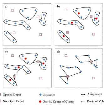
phase, the gravity center of each cluster is calculated which is used to select depot(s) among candidate depots (Figure 2(b)). The clusters are allocated to the opened depot(s) in the third step, considering the distance between the depot and the gravity center of clusters as well as the capacity of the opened depot (Figure 2(c)). Finally, in the fourth phase, ACS forms an admissible tour between each cluster and depot (Figure 2(d)).
The problem is initialized by defining a plane comprising the set of customers, depots, and their coordinate points, namely CUST and DEP, respectively. The heuristic method is repeated for a predefined number of iterations. When the GCM obtained a better solution, it is replaced to the last best known solution. Moreover, since in the first phase of GCM, the first customer at each cluster is selected, randomly, the constituted clusters are different together in each iteration. Thus, the proposed method can search some feasible solutions among all over the solution space. This can help that GCM avoid confining suboptimal solutions. Details of heuristic method are described in following sections.
3.1 Clustering the Customers
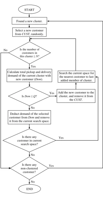
The first phase of GCM is clustering of the customers. The customers are clustered according to the “greedy search algorithm”. At first, to found a cluster, a customer is selected randomly from the set of non-clustered customers belongs to CUST. The algorithm searches for the nearest customer to the last selected customer of the current cluster. The nearest customer is not included to the cluster if either of the following criteria is met: 1) The number of assigned customers to a cluster reached the maximum number of allowed customer per cluster and 2) The total pickup and delivery demand exceeds the remaining capacity of the vehicle. When the number of customer in each cluster reaches to a given number (N), there is no opportunity for any of the customers to enter the current cluster even adding its demand to total demand of cluster is less than the Cap. This is to balance the number of customers in all clusters, which influences
choosing the depots in next phase, and the final solution. The maximum number of members for a cluster is determined using a trial and error method.
Once a new customer is selected to be included to a cluster, total pickup and delivery demands of current members adding to its new member is compared with the capacity of the vehicle (Q). If total demand is less than the Q, the new customer is included in current cluster. Otherwise, last selected customer is withdrawn from the cluster. The greedy search algorithm searches for a new customer close to the last added member of the cluster among the non-clustered customers. This procedure helps to use the maximum capacity of a vehicle. The algorithm founds a new cluster if there is no customer to be assigned to current cluster considering the capacity of vehicle and the maximum number of customers per cluster. When there is no non-clustered customer, the process of clustering stops. Figure 3 illustrates the greedy search algorithm.
3.2 Establishing the Depot(s)
This phase of GCM searches among potential sites to establish proper depot(s). First, the gravity center of clusters is calculated according to equation (20), in which (X(I),Y(I)) is the coordinates of gravity center of cluster I, (xi,yi) is the coordinates of customer i, and nIis the number of customers assigned to cluster I. The gravity center is used as a deputy of the cluster to select the proper depot(s). Choosing the potential site(s) for establishing depot(s) is same as a single facility location problem (SFLP).
I I
i i
I I
i i
I I
n
y
n
x
Y
X
,
,
(20)International Journal of Transportation Engineering, 224 Vol.6/ No.3/ (23) Winter 2019
coordinates of potential site j, (ai,bi) is the coordinates of gravity center of cluster i, m is the number of clusters, and DEP is the number of potential sites.
, :
,...,
m
j i j i j
i
x y Minimize
x a y b
w
j DEP
1
2 2 2
1
1
(21)
The potential sites are sorted in an ascending order and ranked from 1 to DEP according to value of equation (21). Then, the top-ranked potential site is selected to establish. As will be mentioned in next step, if the capacity of the current opened depot is unable to fulfill all clusters, the next potential site of the sorted list is selected to serve the remaining clusters. This procedure (i.e., establishing the depot(s)) is repeated until all clusters are covered.
3.3. Allocating Clusters to Depot(s)
In this phase, the clusters are respectively allocated to the ranked depots. Each depot serves clusters as many as possible, if the next cluster demand does not exceed the remaining capacity of the depot. To allocate the clusters, the Euclidian distance of gravity center of each cluster to the top-ranked depot is calculated. Afterwards, the unassigned clusters are ranked in an ascending order based on the distance of their gravity centers to the depot. The top-ranked cluster is allocated to the top-top-ranked depot. If there is an empty capacity for the top-ranked depot, the second-top-ranked cluster is allocated to the depot. The allocation process to a depot will be finished when there is not enough capacity to allocate new cluster. In this situation, the allocating procedure is repeated for next-ranked depots until all clusters are allocated.
Figure 2. Illustrative example for the greedy clustering method. a)
d) c)
b)
Customer
Not-Open Depot
Opened Depot Assignment
Ali Nadizadeh, Hasan Hosseini Nasab
225 International Journal of Transportation Engineering, Vol.6/ No.3/ (23) Winter 2019
Figure 3. The proposed greedy search algorithm. START
Select a new customer
from CUST, randomly.
Calculate total pickup and delivery demand of the current cluster with
new customer (Dem).
Is Dem ≤ Q?
Is there any non-clustered
customer?
Add the new customer to the cluster, and remove it from
the CUST.
Deduct demand of the selected
customer from Dem and remove
it from the current search space.
Is there any customer in current
search space?
END
Search the current space for the nearest customer to last added member of cluster.
Yes Yes
No No
No
Yes Found a new cluster.
Is the number of customers in
this cluster ≤ N?
International Journal of Transportation Engineering, 226 Vol.6/ No.3/ (23) Winter 2019
3.4
Routing
In the fourth and last phase of GCM, the routing problem for each cluster and its corresponding depot is solved. Each cluster is served by exactly one vehicle, and some vehicles can be supplied by a single depot regarding its capacity. In the routing phase, each cluster with its related depot is considered as a TSP, which is solved by using ant colony system (ACS). ACS is referred to ants’ treatment to find food. The ants spread a material called pheromone and put it on their way so that other ants can pass the same route. The pheromone of shorter route increases and therefore, more ants move from that way. Artificial ants construct a solution by selecting a customer to visit sequentially, until all the customers in a route are visited. Ants select the next customer to visit using a combination of heuristic and pheromone information. A local updating rule is applied to modify the pheromone on the selected route, during the construction of a route. When all ants construct their tours, the amount of pheromone of the best selected route and the global best solution, are updated according to the global updating rule. More details on ACS can be found in [Dorigo and Gambardella, 1996; Bouhafs et al.2010; Abolhoseini and Sadeghi-Niaraki, 2017]. Dorigo et al. [Dorigo and Gambardella, 1996] mentioned that the proper parameters’ values in their proposed heuristic ACS algorithm are α=1, β=5 and ρ=0.65. Hence, these values are used in routing phase of the GCM.
4. Computational Results
To evaluate the efficiency of the proposed GCM, a set of computational experiments are carried out. Since no benchmark instances were publicly available for the CLRP-SPD, Karaoglan et al. used two test sets of CLRP generated by Prodhon [Prodhon, 2008] and Barreto [Barreto, 2003]. They applied demand separation approaches based on Salhi and Nagy [Salhi and Nagy, 1999] and Angelelli and Mansini [Angelelli and Mansini, 2002] to change CLRP instances to CLRP-SPD instances. In this paper, a similar approach like in Karaoglan et al. [Karaoglan et al.2011] is
applied to generate test instances which explain briefly as follows.
In Salhi and Nagy’s approach, a ratio ri =
min(xi/yi;yi/xi), where xi and yi are the coordinates of customer i, is calculated for each customer i, and then the delivery and pickup demands are obtained as di = ⌊ri×qi⌋ and pi = ⌊qi−di⌋, where qi is the demand of customer i. The instances generated by this type are named X. Similarly, another type of instances, called Y, is generated by exchanging delivery and pickup demands of each customer. In Angelelli and Mansini’s approach, the demand of customer i is considered as delivery demand (di = qi) and the pickup demand is generated by pi = ⌊(1−γ)qi⌋ if i is even and pi = ⌊(1+γ)qi⌋ if i is odd. Two γ values as 0.2 and 0.8 are considered to generate two different types of instances called Z and W, respectively. Note that, all benchmark instances and the demand separation approaches described here are adapted to Karaoglan et al. [Karaoglan et al.2011]. Indeed, this is due to the comparison of the proposed method for CLRP-SPD with the previous work seems reasonable.
Ali Nadizadeh, Hasan Hosseini Nasab
227 International Journal of Transportation Engineering, Vol.6/ No.3/ (23) Winter 2019 {a,b} where a = 70 and b = 150. Note that, the
Prodhon’s instances are denoted as |NC|-|N0
|-cluQ [Karaoglan et al.2011].
The first column of the Tables 2 to 5 gives the names of CLRP-SPD instances which explained above. The column named DSS denotes demand separation strategy. Next two columns summarize computational results for the Branch-and-Cut (B&C) algorithm proposed by Karaoglan et al. [Karaoglan et al.2011]. It is important to note that the B&C algorithm have been performed on Intel Xeon 3.16 GHz equipped with 1 GB RAM computer and a time limit of 4 hours has been imposed on each instance. The next two columns show the solution results of instances for the proposed method explained in this paper. The column labeled Gap reports the gap percentage. Note that, the gap percentage for each instance is computed as 100 × [(OFVGCM – OFVB&C)/ OFVB&C] where OFVGCM and OFVB&C are denoted as objective function value of GCM and B&C algorithm, respectively. Since to the best our knowledge there is only one approach in this research area, the performance of our approach has been compared to B&C algorithm.
For convenience, Table 6 has summarized the results of Tables 2 to 5. Comparison between the solutions of GCM and B&C algorithm, Table 6 readily reveals that the GCM has improved 95 instances out of 148. Also, while the GCM has solved 14 instances without any changes in solution values, 39 of them have failed to compete with the results of B&C algorithm. Eventually, the proposed GCM is competitive with B&C algorithms in terms of solution quality by providing the 95 new bestknown solutions and total average gap of -4.77%. Further performance of the proposed GCM against the B&C algorithm is related to the solving time of instances. In Table 6, it can
be seen that the GCM has solved all instances with the average solving time of 160.86 seconds. But, this value for the B&C algorithm with the mentioned quality of answers is equal to 9221.01 seconds. This comparison easily shows that the GCM has lower running time than the B&C algorithm. So, the GCM can also be considered more efficient than the B&C algorithm in terms of solving time of instances.
Further results of the numerical experiment for evaluating the efficiency of GCM is shown in Table 7. The efficiency of the proposed method is carried out by using 19 standard benchmark test problems of CLRP presented by [Barreto, 2003]. It is noted that, each test problem of CLRP-SPD can be reduced to a CLRP. Actually, if the pickup demands equal 0, then the CLRP-SPD is changed to CLRP. The comparative results are summarized in Table 7. First column of the Table 7 represents the ID number of each test problem. Second column reports the best-known solutions (BKS) that are given in the literature [Lopes et al.2016]. The solutions and CPU times obtained by two approaches: the clustering based heuristic (CH) [Barreto et al. 2007] and HybPSO-LRP [Marinakis and Marinaki, 2008] are shown in next columns. Last column of the table shows the solution and CPU time of the heuristic algorithm.
International Journal of Transportation Engineering, 228 Vol.6/ No.3/ (23) Winter 2019
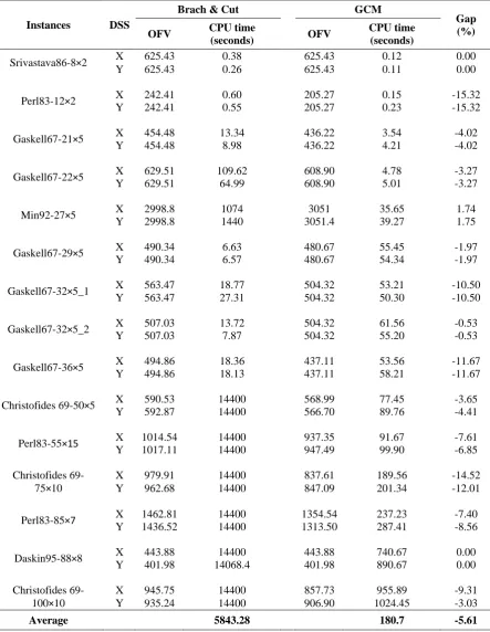
Table 2. Computational results for the instances derived from Barreto’s test set by Salhi and Nagy’s separation approach.
Instances DSS
Brach & Cut
GCM
Gap (%)
OFV CPU time
(seconds) OFV
CPU time (seconds)
Srivastava86-8×2 X 625.43 0.38 625.43 0.12 0.00
Y 625.43 0.26 625.43 0.11 0.00
Perl83-12×2 X 242.41 0.60 205.27 0.15 -15.32
Y 242.41 0.55 205.27 0.23 -15.32
Gaskell67-21×5 X 454.48 13.34 436.22 3.54 -4.02
Y 454.48 8.98 436.22 4.21 -4.02
Gaskell67-22×5 X 629.51 109.62 608.90 4.78 -3.27
Y 629.51 64.99 608.90 5.01 -3.27
Min92-27×5 X 2998.8 1074 3051 35.65 1.74
Y 2998.8 1440 3051.4 39.27 1.75
Gaskell67-29×5 X 490.34 6.63 480.67 55.45 -1.97
Y 490.34 6.57 480.67 54.34 -1.97
Gaskell67-32×5_1 X 563.47 18.77 504.32 53.21 -10.50
Y 563.47 27.31 504.32 50.30 -10.50
Gaskell67-32×5_2 X 507.03 13.72 504.32 61.56 -0.53
Y 507.03 7.87 504.32 55.20 -0.53
Gaskell67-36×5 X 494.86 18.36 437.11 53.56 -11.67
Y 494.86 18.13 437.11 58.21 -11.67
Christofides 69-50×5 X 590.53 14400 568.99 77.45 -3.65
Y 592.87 14400 566.70 89.76 -4.41
Perl83-55×15 X 1014.54 14400 937.35 91.67 -7.61
Y 1017.11 14400 947.49 99.90 -6.85
Christofides 69-75×10
X 979.91 14400 837.61 189.56 -14.52
Y 962.68 14400 847.09 201.34 -12.01
Perl83-85×7 X 1462.81 14400 1354.54 237.23 -7.40
Y 1436.52 14400 1313.50 287.41 -8.56
Daskin95-88×8 X 443.88 14400 443.88 740.67 0.00
Y 401.98 14068.4 401.98 890.67 0.00
Christofides 69-100×10
X 945.75 14400 857.73 955.89 -9.31
Y 935.24 14400 906.90 1024.45 -3.03
Ali Nadizadeh, Hasan Hosseini Nasab
229 International Journal of Transportation Engineering, Vol.6/ No.3/ (23) Winter 2019
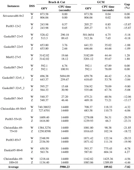
Table 3. Computational results for the instances derived from Barreto’s test set by Angelelli and Mansini’s separation approach.
Instances DSS
Brach & Cut
GCM
Gap (%)
OFV CPU time
(seconds) OFV
CPU time (seconds)
Srivastava86-8×2 W 873.58 0.00 873.58 0.04 0.00
Z 806.06 0.00 806.06 0.02 0.00
Perl83-12×2 W 243.98 0.57 205.27 0.85 -15.87
Z 243.98 0.65 205.27 0.71 -15.87
Gaskell67-21×5 W 528.42 290.18 501.0654 6.75 -5.18
Z 513.3 89.43 512.36 7.65 -0.18
Gaskell67-22×5 W 653.80 3.76 641.53 35.02 -1.88
Z 653.80 2.66 646.66 44.66 -1.09
Min92-27×5 W 3142.02 19.66 3182.09 44.44 1.28
Z 3142.02 18.12 3201.12 55.67 1.88
Gaskell67-29×5 W 592.1 6.76 592.1 67.89 0.00
Z 592.1 100.91 592.1 78.09 0.00
Gaskell67-32×5_1 W 696.38 5694.09 659.78 46.42 -5.26
Z 643.37 259.67 618.65 53.78 -3.84
Gaskell67-32×5_2 W 595.27 15.68 536.92 70.09 -9.80
Z 564.33 30.90 535.68 67.76 -5.08
Gaskell67-36×5 W 540.37 27.20 475.21 60.56 -12.06
Z 540.37 46.46 469.18 73.21 -13.17
Christofides 69-50×5 W 740.38832 14400 708.37 118.33 -4.32
Z 727.6701 14400 683.58 110.75 -6.06
Perl83-55×15 W 1609.40 14400 1278.08 56.31 -20.59
Z 1616.80 14400 1239.93 66.3 -23.31
Christofides 69-75×10
W 1384.3276 14400 1081.80 98.38 -21.85
Z 1250.8598 14400 1016.65 102.34 -18.72
Perl83-85×7 W 2348.99 14400 1871.42 122.34 -20.33
Z 2336.50 14400 1871.42 111.34 -19.90
Daskin95-88×8 W 650.50 14400 593.37 775.45 -8.78
Z 563.76 14400 587.81 604.34 4.27
Christofides 69-100×10
W 1218.44 14400 1162.82 1425.36 -4.56
Z 1134.40 14400 1083.86 1389.89 -4.46
Average 5980.23 189.82 -7.82
Table 4. Results for instances derived from Prodhon’s test set by Salhi and Nagy’s separation approach.
Instances DSS Brach & Cut GCM Gap (%)
OFV CPU time (seconds) OFV CPU time (seconds)
International Journal of Transportation Engineering, 230 Vol.6/ No.3/ (23) Winter 2019
Y 16816.00 73.77 16823.24 3.41 0.04
20-5-1b X 9167.14 1.86 9167.14 5.63 0.00
Y 9167.14 0.27 9167.14 6.21 0.00
20-5-2a X 17814.7 27.93 17808.40 2.14 -0.04
Y 17814.7 16.02 17808.40 3.56 -0.04
20-5-2b X 10257.30 1.61 10257.30 5.32 0.00
Y 10257.30 1.38 10257.30 4.9 0.00
50-5-1a X 16377.80 14400 16403.18 62.92 0.15
Y 16391.18 14400 16409.21 79.55 0.11
50-5-1b X 13138.15 14400 13184.45 127.78 0.35
Y 13138.15 14400 13168.35 134.54 0.23
50-5-2a X 26419.36 14400 26462.04 59.01 0.16
Y 26419.09 14400 26461.13 67.6 0.16
50-5-2b X 22268.50 213.75 22304.80 99.5 0.16
Y 22268.50 1147.76 22312.05 107.43 0.20
50-5-3a X 11652.09808 14400 11650.85 66.43 -0.01
Y 11655.6665 14400 11666.86 71.90 0.10
50-5-3b X 8482.56 14400 8542.07 122.45 0.70
Y 8472.41 14400 8512.53 132.56 0.47
100-5-1a X 102572.30 14400 101660.86 88.45 -0.89
Y 102555.05 14400 101659.05 104.65 -0.87
100-5-1b X 94997.86 14400 94041.51 211.65 -1.01
Y 94992.65 14400 94045.16 241.12 -1.00
100-5-2a X 105771.22 14400 104781.10 98.11 -0.94
Y 105771.22 14400 104806.90 90.76 -0.91
100-5-2b X 97291.57104 14400 96304.12 289.06 -1.01
Y 97274.0442 14400 96390.14 255.6 -0.91
100-5-3a X 56648.23857 14400 57699.55 79.98 1.86
Y 56706.38018 14400 57681.65 95.39 1.72
100-5-3b X 50279.84706 14400 50305.90 266.89 0.05
Y 50265.99872 14400 50305.70 255.11 0.08
100-10-1a X 110959.70 14400 110063.57 110.56 -0.81
Y 110961.72 14400 110086.83 123.3 -0.79
100-10-1b X 102511.94 14400 102580.00 301.23 0.07
Y 102497.70 14400 102581.56 298.5 0.08
100-10-2a X 204974.95 14400 105740.61 130.34 -48.41
Y 109639.16 14400 105708.27 125.45 -3.59
100-10-2b X 100210.81 14400 98255.80 310.89 -1.95
Y 100209.09 14400 98304.60 331.23 -1.90
100-10-3a X 101819.79 14400 99963.24 145.69 -1.82
Y 100243.3149 14400 99849.24 130.13 -0.39
100-10-3b X 93515.92 14400 93522.97 335.1 0.01
Y 93568.48 14400 93537.50 368.8 -0.03
Ali Nadizadeh, Hasan Hosseini Nasab
231 International Journal of Transportation Engineering, Vol.6/ No.3/ (23) Winter 2019
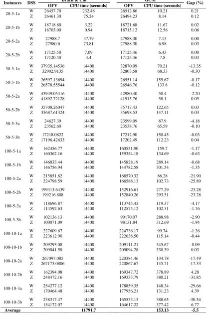
Table 5. Results for instances derived from Prodhon’s test set by Angelelli and Mansini’s separation.
Instances DSS Brach & Cut GCM Gap (%)
OFV CPU time (seconds) OFV CPU time (seconds)
20-5-1a W 26457.70 232.48 26512.86 10.21 0.21
Z 26461.30 75.24 26494.23 8.14 0.12
20-5-1b W 18718.80 3.22 18721.68 11.67 0.02
Z 18703.00 0.94 18715.12 12.56 0.06
20-5-2a W 27988.7 37.79 27988.30 7.13 0.00
Z 27980.6 73.81 27988.30 6.98 0.03
20-5-2b W 17125.50 7.09 17125.46 6.43 0.00
Z 17120.50 4.4 17125.46 7.8 0.03
50-5-1a W 37935.14536 14400 32870.09 70.21 -13.35
Z 32902.9135 14400 32803.58 68.33 -0.30
50-5-1b W 26597.13694 14400 26551.14 155.67 -0.17
Z 26578.55544 14400 26546.76 133.8 -0.12
50-5-2a W 43949.05416 14400 42980.40 50.4 -2.20
Z 41892.72128 14400 41915.76 58.1 0.05
50-5-2b W 35708.26047 14400 35717.43 122.65 0.03
Z 35687.61324 14400 35698.53 147.11 0.03
50-5-3a W 24627.39 14400 23599.09 87.9 -4.18
Z 23562.60 14400 23538.76 65.59 -0.10
50-5-3b W 17218.0822 14400 17212.90 150.45 -0.03
Z 17196.42633 14400 17202.49 112.23 0.04
100-5-1a W 162456.77 14400 160551.90 159.7 -1.17
Z 160362.16 14400 159354.18 134.69 -0.63
100-5-1b W 146833.44 14400 145828.19 289.14 -0.68
Z 146756.94 14400 144782.58 301.54 -1.35
100-5-2a W 215851.62 14400 168570.32 86.28 -21.90
Z 224798.59 14400 166588.13 102.73 -25.89
100-5-2b W 199313.6439 14400 152916.61 277.29 -23.28
Z 199216.808 14400 152840.26 293.51 -23.28
100-5-3a W 118696.87 14400 113745.43 119.37 -4.17
Z 114592.63 14400 112575.12 102.31 -1.76
100-5-3b W 102136.13 14400 99170.07 288.98 -2.90
Z 100071.09 14400 98131.84 312.69 -1.94
100-10-1a W 227609.67 14400 224736.17 99.74 -1.26
Z 223612.90 14400 222638.50 115.14 -0.44
100-10-1b W 209293.08 14400 209111.21 345.67 -0.09
Z 209041.58 14400 209094.28 330.39 0.03
100-10-2a W 267097.085 14400 220384.46 134.78 -17.49
Z 267173.0806 14400 220867.67 145.71 -17.33
100-10-2b W 162394.08 14400 169347.72 378.89 4.28
Z 248472.16 14400 169333.79 380.21 -31.85
100-10-3a W 254277.12 14400 178859.35 148.34 -29.66
Z 170464.48 14400 177956.21 131.23 4.39
100-10-3b W 238317.47 14400 165533.13 388.65 -30.54
Z 154172.07 14400 164617.22 377.42 6.77
International Journal of Transportation Engineering, 232 Vol.6/ No.3/ (23) Winter 2019
Table 6. Summarized of the computational results between GCM and B&C algorithm.
Test set DSS No. of
instances
Statues of GCM results against B&C
Average of CPU time
(seconds) Average of
Gap (%)
Improved Unchanging Worsened Brach & Cut GCM
Barreto X 15 24 4 2 5843.28 180.7 -5.61
Y 15
Barreto W 15 23 4 3 5980.23 189.82 -7.82
Z 15
Prodhon X 22 20 4 20 11162.93 135.31 -1.38
Y 22
Prodhon W 22 28 2 14 11791.7 153.13 -5.5
Z 22
Total 148 95 14 39
Average
9221.01 160.86 -4.77
Table 7. Computational results of heuristic algorithm on standard test problems of CLRP.
GCM HybPSO-LRP CH BKS CLRP instance Gap (%) Solution Gap (%) Solution Gap (%) Solution 0.00 565.6 3.02 582.7 3.02 582.7 565.6 Christ69–50×5 4.96 886.3 4.96 886.3 4.96 886.3 844.4 Christ69–75×10 0.00 833.9 6.66 889.4 6.66 889.4 833.9 Christ69–100×10 0.66 427.7 1.88 432.9 2.59 435.9 424.9 Gaskell67–21×5 1.09 591.5 0.58 588.5 1.09 591.5 585.1 Gaskell67–22×5 0.00 512.1 0.00 512.1 0.00 512.1 512.1 Gaskell67–29×5 0.00 562.2 1.53 570.8 1.69 571.7 562.2 Gaskell67–32×5 0.00 504.3 1.35 511.1 1.41 511.4 504.3 Gaskell67–32×5 1.91 469.2 2.24 470.7 2.24 470.7 460.4 Gaskell67–36×5 0.64 205.3 0.00 204 0.00 204 204 Perl83–12×2 1.35 1127.1 2.14 1135.9 2.17 1136.2 1112.1 Perl83–55×15 0.00 1622.5 2.12 1656.9 2.12 1656.9 1622.5 Perl83—85×7 4.22 580791.5 4.20 580680.2 4.20 580680.2 557275.2 Perl83—318×4 0.00 670118.5 11.57 747619 11.57 747619 670118.5 Perl83—318×4 8.18 384.9 8.18 384.9 8.18 384.9 355.8 Dasnki95–88×8 6.20 46642.7 6.20 46642.7 6.20 46642.7 43919.9 Dasnki95–150×10 0.00 3062 0.00 3062 0.00 3062 3062 Min92–27×5 9.11 6229 9.13 6230 9.27 6238 5709 Min92–134×8 0.00 12290.3 1.50 12474.2 1.50 12474.2 12290.3 Or76–117×14 2.02 3.54 3.62 Avg.
233 International Journal of Transportation Engineering, Vol.6/ No.3/ (23) Winter 2019
5. Conclusion
Logistics costs often represent a large part of the cost of companies. In order to reduce them, facility location and vehicle routing are crucial. In the management decision of the logistics, facility location problems and vehicle routing problems are interdependent. But often, they are considered separately and sometimes increase the total cost. This paper contributes to the capacitated location-routing problem with simultaneous pickup and delivery. A node-based MIP formulation for the CLRP-SPD based on Karaoglan et al. [Karaoglan et al.2012] is proposed. To solve the problem, a GCM with four phases was proposed where greedy search algorithm was applied to cluster the customers in first phase. Next phase determined the gravity centers of cluster to select the appropriate depot(s). Clusters of customer were assigned to selected depot(s) in the third phase. In the fourth phase the routes between depot(s) and assigned clusters were built by ant colony system. Comparisons of the results of the GCM with the B&C algorithm obtained from the literature of the CLRP-SPD showed that the efficiency of the proposed method was satisfactory. In 95 instances out of 148, the GCM found better solutions. While the total average gap of instances was -4.77%, the GCM also solved all instances in lower solving time compared to the B&C algorithm. Finally, it is concluded that the GCM is more effective than the B&C algorithm in terms of solution quality and solving time of instances. This paper has some capable future research directions: considering the CLRP-SPD with fuzzy pickup and delivery demands, developing other solution algorithms e.g. hybrid evolutionary algorithms, and developing the model by some more realistic assumptions e.g. heterogeneous vehicles with unequal capacities.
6. References
-Angelelli, E. and Mansini, R. (2002) "The vehicle routing problem with time windows and simultaneous pick-up and delivery. In: Lecture Notes in Economics and Mathematical Systems", Springer, Germany, pp. 249–267.
-Barreto, S. (2003)
"http://sweet.us.pt/_iscf143".
-Barreto, S., Ferreira, C., Paixao, J. and Sousa Santos, B. (2007) "Using clustering analysis in a capacitated location-routing problem", European Journal of Operational Research, Vol. 179, pp. 968-977.
-Belenguer, J. M., Benavent, E., Prins, C., Prodhon, C. and Wolfler-Calvo, R. (2011) "A Branch-and-cut method for the Capacitated Location-Routing Problem", Computers and Operations Research, Vol. 38 pp. 931-941.
-Bouhafs, L., Hajjam, A. and Koukam, A. (2010) "A hybrid heuristic approach to solve the capacitated vehicle routing problem", Journal of Artificial Intelligence: Theory and Application, Vol. 1, No. 1, pp. 31-34.
-Catay, B. (2010) "A new saving-based ant algorithm for the Vehicle Routing Problem with Simultaneous Pickup and Delivery", Expert Systems with Applications, Vol. 37, pp. 6809– 6817.
-Derbel, H., Jarboui, B., Hanafi, S. and Chabchoub, H. (2012) "Genetic algorithm with iterated local search for solving a location-routing problem", Expert Systems with Applications, Vol. 39, pp. 2865-2871.
-Dorigo, M. and Gambardella, L. M. (1996) "A study of some properties of ant-Q", PPSN, springer-Verlag, Berlin, pp. 656-665.
-Drexl, M. and Schneider, M. (2015) "A survey of variants and extensions of the location-routing problem", European Journal of Operational Research, Vol. 241, No. 2, pp. 283-308.
-Duhamel, C., Lacomme, P., Prins, C. and Prodhon C. (2010) "A GRASP×ELS approach for the capacitated location-routing problem", Computers & Operations Research, Vol. 37, pp. 1912-1923.
International Journal of Transportation Engineering, 234 Vol.6/ No.3/ (23) Winter 2019
the multi-depot vehicle routing problem", 4OR, Vol. 12, No. 1, pp. 99-100.
-Ghatreh Samani, M. and Hosseini-Motlagh, S.-M. (2017) "A hybrid algorithm for a two-echelon location- routing problem with simultaneous pickup and delivery under fuzzy demand", International Journal of Transportation Engineering, Vol. 5, No. 1, pp. 59-85.
-Huang, S.-H. (2015) "Solving the multi-compartment capacitated location routing problem with pickup–delivery routes and stochastic demands", Computers & Industrial Engineering, Vol. 87, pp. 104-113.
-Karaoglan, I., Altiparmak, F., Kara, I. and Dengiz, B. (2011) "A branch and cut algorithm for the location-routing problem with simultaneous pickup and delivery", European Journal of Operational Research, Vol. 211, pp. 318-332.
-Karaoglan, I., Altiparmak, F., Kara, I. and Dengiz, B. (2012) "The location-routing problem with simultaneous pickup and delivery: Formulations and a heuristic approach", Omega, Vol. 40, No. 4, pp. 465-477.
-Laporte, G. (1988) "Location-routing problems. Vehicle Routing: Methods and Studies", B. L. In: Golden, Assad, A.A. (Eds.). North-Holland, Amsterdam, pp. 163–198.
-Lopes, R. B., Ferreira, C. and Santos, B. S. (2016) "A simple and effective evolutionary algorithm for the capacitated location–routing problem", Computers & Operations Research, Vol. 70, pp. 155-162.
-Manzour-al-Ajdad, S. M. H., Torabi, S. A. and Salhi, S. (2012) "A hierarchical algorithm for the planar single-facility location routing problem", Computers & Operations Research, Vol. 39, pp. 461-470.
-Marinakis, Y. and Marinaki, M. (2008) "A Particle Swarm Optimization Algorithm with Path Relinking for the Location Routing Problem", Journal of Mathematical Modelling and Algorithm, Vol. 7, pp. 59–78.
-Min, H., Jayaraman, V. and Srivastava, R. (1998) "Combined location-routing problems: A synthesis and future research directions", European Journal of Operational Research, Vol. 108, pp. 1–15.
-Nadizadeh, A. (2017) "The fuzzy multi-depot vehicle routing problem with simultaneous pickup and delivery: Formulation and a heuristic algorithm", International Journal of Industiral Engineering & Producion Research, Vol. 28, No. 3, pp. 325-345.
-Nadizadeh, A. and Kafash, B. (2017) "Fuzzy capacitated location-routing problem with simultaneous pickup and delivery demands", Transportation Letters, DOI: 10.1080/19427867.2016.1270798.
-Nadizadeh, A. and Hosseini Nasab, H. H. (2014) "Solving the dynamic capacitated location-routing problem with fuzzy demands by hybrid heuristic algorithm", European Journal of Operational Research, Vol. 238, No. 2, pp. 458-470.
-Nadizadeh, A., Sadegheih, A. and Sabzevari Zadeh, A. (2017) "A hybrid heuristic algorithm to solve capacitated location-routing problem with fuzzy demands", International Journal of Industrial Mathematics, Vol. 9, No. 1, pp. 1-20.
-Nadizadeh, A., Sahraeian, R., Sabzevari Zadeh, A. and Homayouni, S. M. (2011) "Using greedy clustering method to solve capacitated location-routing problem", African Journal of Business Management, Vol. 5, No. 17, pp. 7499-7506.
-Nagy, G. and Salhi, S. (2007) "Location-routing: Issues, models and methods", European Journal of Operational Research, Vol. 177, pp. 649-672.
-Prins, C., Prodhon, C. and Wolfler Calvo, R. (2006) "Solving the capacitated location-routing problem by a GRASP complemented by a learning process and a path relinking", Operational Research Quarterly, Vol. 4, pp. 221-238.
Ali Nadizadeh, Hasan Hosseini Nasab
235 International Journal of Transportation Engineering, Vol.6/ No.3/ (23) Winter 2019 "http://prodhonc.free.fe/homepage".
-Prodhon, C. and Prins, C. (2014) "A survey of recent research on location-routing problems", European Journal of Operational Research, Vol. 238, No. 1, pp. 1-17.
-Rahmani, Y., Cherif-Khettaf, W. R. and Oulamara, A. (2015) "A local search approach for the two–echelon multi-products location– routing problem with pickup and delivery", IFAC-Papers On Line, Vol. 48, No. 3, pp. 193-199.
-Rahmani, Y., Ramdane Cherif-Khettaf, W. and Oulamara, A. (2016) "The two-echelon multi-products location-routing problem with pickup and delivery: formulation and heuristic approaches", International Journal of Production Research, Vol. 54, No. 4, pp. 999-1019.
-Rath, S. and Gutjahr, W. J. (2014) "A math-heuristic for the warehouse location–routing problem in disaster relief", Computers & Operations Research, Vol. 42, pp. 25–39.
-Salhi, S. and Nagy, G. (1999) "Consistency and robustness in location routing", Studies in Locational Analysis, Vol. 13, pp. 3-19.
-Salhi, S. and Rand, G. K. (1989) "The effect of ignoring routes when locating depots", European Journal of Operational Research, Vol. 39, pp. 150–156.
-Tavakkoli-Moghaddam, R., Razie, Z. and Tabrizian, S. (2016) "Solving a Bi-Objective Multi-Product Vehicle Routing Problem with Heterogeneous Fleets under an Uncertainty Condition", International Journal of Transportation Engineering, Vol. 3, No. 3, pp. 207-225.
-Wang, X. and Li, X. (2017) "Carbon reduction in the location routing problem with heterogeneous fleet, simultaneous pickup-delivery and time windows", Procedia Computer Science, Vol. 112, pp. 1131-1140.
-Webb, M. H. J. (1968) "Cost functions in the
location of depots for multiple delivery journeys", Operational Research Quarterly, Vol. 19, No. 3, pp. 311-320.
-Yang, J. and Sun, H. (2015) "Battery swap station location-routing problem with capacitated electric vehicles", Computers & Operations Research, Vol. 55, pp. 217-232.
-Yu, V. F. and Lin, S.-W. (2014) "Multi-start simulated annealing heuristic for the location routing problem with simultaneous pickup and delivery", Applied Soft Computing, Vol. 24, pp. 284-290.
-Yu, V. F. and Lin, S.-Y. (2016) "Solving the location-routing problem with simultaneous pickup and delivery by simulated annealing", International Journal of Production Research, Vol. 54, No. 2, pp. 526-549.
-Zarandi, M., Hemmati, A., Davari S. and Turksen, I. (2013) "Capacitated location-routing problem with time windows under uncertainty", Knowledge-Based Systems, Vol. 37, pp. 480–489.
-Zarandi, M. H. F., Hemmati, A. and Davari, S. (2011) "The multi-depot capacitated location-routing problem with fuzzy travel times", Expert Systems with Applications, Vol. 38, No. 8, pp. 10075-10084.
-Zare Mehrjerdi, Y. and Nadizadeh, A. (2013) "Using greedy clustering method to solve capacitated location-routing problem with fuzzy demands." European Journal of Operational Research, Vol. 229, No. 1, pp. 75-84.
Zare Mehrjerdi, Y. and Nadizadeh, A. (2016) "Heuristic Method to Solve Capacitated Location-Routing Problem with Fuzzy Demands", International Journal of Industiral Engineering & Producion Research, Vol. 27, No. 1, pp. 1-19.