Traffic Condition Detection in Freeway by using Autocorrelation of Density and Flow

85 International Journal of Transportation Engineering, Vol.6/ No.1/ Summer 2018 Hamid Torfehnejad1, Ali Jalali2

Received: 13. 03. 2017 Accepted: 30. 07. 2017

Abstract

Traffic conditions vary over time, and therefore, traffic behavior should be modeled as a stochastic process. In this study, a probabilistic approach utilizing Autocorrelation is proposed to model the stochastic variation of traffic conditions, and subsequently, predict the traffic conditions. Using autocorrelation of the time series samples of density and flow which are collected from segments with predefined specifications is the main technique to detect the trend in flow and density changes if exist. A table of possibilities for flow and density changes in two sequential segments will help to detect congestion or any other abnormal traffic events.

In this study proposes a stochastic approach to predict the traffic situation in freeway. The dynamic changes of freeway traffic conditions are addressed with state transition probabilities. For sequence trends of density and flow change, using autocorrelation of speed and flow series will estimate the most likely sequence of traffic states. This is the novelty in this paper that introduces a robust method to recognize the traffic state in a segmented freeway. According to the model definitions 3-state traffic pattern prediction implemented as No Risk (NR), Risk (R) and High risk (HR). We evaluated the proposed method using different data sources of real traffic scenes from Tehran-Qom freeway, Iran. A total of 480 minutes, which corresponds to interstate highways, are chosen for testing. The number of passed vehicle and mean speed are collected by six traffic counter every 1 minute. The estimation rate of this model is 95% over a short time periodfor the month of July 2014.

Keywords: Flow, density, autocorrelation, traffic detection, prediction

Corresponding author E-mail: [email protected]

1.

Introduction

Delays and congestion are two of the most important issues in traffic engineering studies. However, there is still congestion and delays for various reasons. Traffic events can be diagnosed by imaging cameras or by automatic incident detection algorithms (AID), which they have received their information from the several kinds of detectors. In classical approach the infrastructure plays the role of event detector like magnetic loops under road Surface camera and other kinds of sensors on road side. Collected information is transmitted to traffic management centers and after processing data, information is provided to road users mainly using VMS and RDS-TMC.Active traffic management (ATM) is the ability to dynamically manage recurrent and non-recurrent congestion based on prevailing and predicted traffic conditions. Focusing on trip reliability, it maximizes the effectiveness and efficiency of the facility. It increases throughput and safety through the use of integrated systems with new technology, including the automation of dynamic deployment to optimize performance quickly and without delay that occurs when operators must deploy operational strategies manually. ATM approaches focus on influencing travel behavior with respect to

lane/facility choices and

operations. ATM strategies can be deployed singularly to address a specific need such as the utilizing adaptive ramp metering to control traffic flow or can be combined to meet system-wide needs of congestion management, traveler information, and safety resulting in synergistic performance gains [ Kurzhanskiy and Varaiya, 2010].

Mathematical description of traffic flow has been a lively subject to research. The traffic flow theory is a science, which has addressed questions related to understanding traffic

process and optimizing these processes through proper design and control [Hoogendoorn and Bovy, 2001]. During the past fifty years, a wide range of traffic flow theories and models have been developed. The models can be classified according to:

 Scales of the independent variables (continuous, discrete, semi-discrete).

 Representation of the processes (deterministic,stochastic).

 Level of detail (microscopic with high detail, mesoscopic with medium detail, macroscopic with low detail) [Yang and Sahli, n.d.]

87 International Journal of Transportation Engineering, Vol.6/ No.1/ Summer 2018 Definitions (Free Flow), heavy (Synchronized

Flow) and dense (Wide Moving Jam ) as they are.[Kerner, 2013] In this research a simplified model will be used with no on-ramps and off-on-ramps or road junctions. This is a valid assumption for a freeway stretch between two road junctions or for an inter-urban freeway with small in and out traffic along its length. If this assumption does not hold, additional measures, such as ramp metering, may be necessary.

2.

Literature Review and Traffic

Models

So many researchers had studied the problem of reliable incident detection on freeway and had developed a number of automatic detection systems using different equipment live loop detectors, camera, or IntelliDrive-based probe vehicles. [Willsky et al. and Qiu et al. 2010]. Some other researchers have developed different algorithms to predict the traffic flow or other algorithms for dynamic speed management in segmented freeways. [Torfehnejad, 2011] develoed a realistic and practical method of dynamic speed limit control based on an operational macroscopic traffic flow simulation model which requires relatively less data collection efforts.. Such a solution reduces the cost of communication and the on-line computational load, and increases the modularity and scalability of the system. An accurate prediction of traffic parameters can help improve the transportation system functions with respect to real-time control strategies, advance warning in monitoring systems, as well as reduction of congestion, delay, and energy consumption. [Porikli and Li, 2004] Predictive information is essential to both transportation system users and providers for better decision making that could improve the productivity of the transportation system and reduce the direct and indirect cost of both

the field of AI. The AI techniques that are applied to incident detection include the artificial neural networks (ANN) [Abdulhai and Ritchie, 1999; Ishak and Al-Deek, 1999], the fuzzy logic [Chang and Wang, 1995], and the combined fuzzy logic and ANN [Hsiao et al. 1994]. It can be seen from the listed references above that most of the neural network models have been tested in the studies for incident detection. In macroscopic algorithms, macroscopic traffic variables are used in incident detection. These algorithms include the multiple model algorithm [Willsky et al. 1980] and the generalized likelihood ratio algorithm [Willsky et al. 1980]. Wavelet algorithms are the recent developments in freeway incident detection algorithms. In [Adeli and Karim 2000], wavelet transform was used with a fuzzy data clustering method for feature extraction. This feature extraction was integrated with the radial basis function neural network (RBFNN) for incident detection. In general, the wavelet was viewed as a means to denoise the traffic measurements in these studies.

In microscopic models, individual vehicles are modeled along with their interaction with other vehicles and the road network. These individual vehicles adjust their speeds and lanes and the interaction of all vehicles models the resulting traffic in the network. Macroscopic models ignore these individual vehicle interactions and represent the aggregate dynamic properties of a group of vehicles, usually represented as a continuum. Most macroscopic models represent traffic as a compressible fluid, and describe the density, flow and speed evolution using dynamic equations. Many different traffic flow models have been developed since the first attempts in 1930. Mesoscopic models imply an aggregation level halfway between the microscopic and macroscopic families. The Lighthill Whitham Richards model, commonly known as the LWR model, is a first order model described by the vehicle conservation equation. The Cell

Transmission Model (CTM) as a first order discrete dynamic model which is consistent with the hydrodynamic theory of the LWR model [Daganzo, 1995]. The CTM can be interpreted as the discretization of the LWR model with a time step of Ts and uniform sections with length L, according to L = Tsvf , where vf is the free-flow speed. The uniform sections are known as cells, and they are increasingly numbered from upstream to downstream. The main assumption in the first order models is the existence of a static density flow relationship, which also implies a static speed-density relationship. Greenshields was the first to propose a parabolic fundamental diagram from observations of traffic along a two lane highway. [Golob et al. 2007] used Autocorrelations, the correlation of a variable at one 30-s interval with the value of the same variable in the previous 30-s interval, for all adjacent time intervals in the 20-min period of traffic condition as one of the parameters to evaluate highway safety performance. The right aim in this research is using autocorrelation function to evaluate the condition of trend changes in flow and density. In fact we use autocorrelation factor to detect the direction of changes in time series of flow and density in order to detect the traffic condition in each segment in a segmented freeway.

3.

Methodology

3.1

Definitions

89 International Journal of Transportation Engineering, Vol.6/ No.1/ Summer 2018 addressed with state transition probabilities.

For a sequence of density and flow change trends, HMMs estimate the most likely sequence of traffic states.

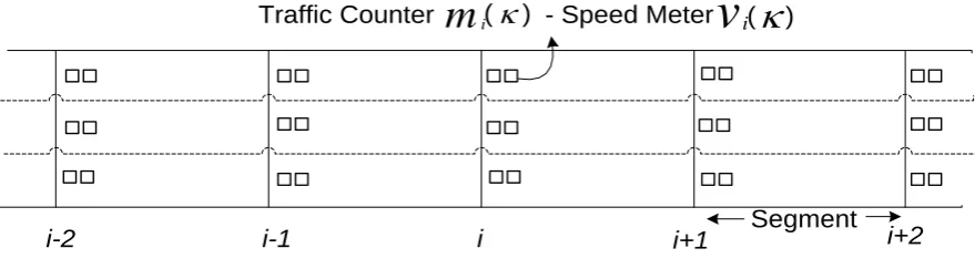
In this scenario we assume that the minimum local equipment is present to collect the required data. As it shows in Figure 1, we have just a couple of loop detectors per lane or any other traffic counter system at the start point of each segment, so we can collect the time mean speed 𝑣_𝑖(𝑘) and the number of passed vehicles𝑚𝑖(𝑘), related to each segment in each time interval(𝜏) .

The following equations are defined:

𝐿 = Segment length, 𝑇 =Time period of the algorithm,

𝜏=Data acquisition time interval (time step)

𝑚𝑖(𝑘)Total number of passed vehicles in all lanes at segment 𝑖 in 𝑘th time step.

𝑢_𝑖(𝑘)= 1

𝑚𝑖(𝑘)∑ 𝑢𝑛

𝑚𝑖

𝑛=1 Time mean speed of all vehicles at segment 𝑖 in 𝑘th time step

𝑢𝑛 = Speed of 𝑛th vehicle passed in segment 𝑖 in 𝑘th time step

𝑣𝑖(𝑘)= 1 1 𝑚𝑖(𝑘)∑𝑚𝑖(𝑘)𝑛=1 𝑡𝑛(𝑘)

Space mean speed of all

vehicles at segment 𝑖 in 𝑘th time step

𝑡_𝑛(𝑘) = Travel time of 𝑛th vehicle passed in segment 𝑖 in 𝑘th time step

𝑞𝑖(𝑘) =𝑚𝑖_𝑇(𝑘)Traffic flow of vehicles passing segment i as a reference point in a time step τ

𝜌_𝑖(𝑘) = 𝑞_𝑖(𝑘) /𝑣_𝑖(𝑘) Traffic density at segment 𝑖 in kth time step

∆𝜌_𝑖(𝑘) = 𝑚𝑖+1(𝑘) − 𝑚𝑖(𝑘) Density variation at segment 𝑖 in kth time step

∆𝑞𝑖(𝑘) = 𝑞𝑖+1(𝑘) − 𝑞𝑖(𝑘) Flow variation at segment 𝑖 in kth time step

In this paper a simplified model is used with no on-ramps and off-ramps or road junctions. Although some parameters have critical role in road traffic condition like FIFO (First In First Out), merge, diverge, ramp, lane change and length of cell, this is a valid assumption for a freeway stretch between two road junctions or for an inter-urban freeway with small in and out traffic along its length. If this assumption does not hold, additional measures such as ramp metering may be necessary. The model represents a freeway stretch of 𝑁 segments, each of length 𝐿[𝑘𝑚] and 𝜆 number of lanes. The vehicles enter the stretch at segment 1 (upstream) and leave it from segment N

downstream. The mean vehicle density 𝜌𝑖 (𝑣𝑒ℎ/ 𝑘𝑚), mean traffic flow 𝑞𝑖 (𝑣𝑒ℎ/ℎ) and time mean speed 𝑣𝑖 (km/h) for each segment are the discrete state variables and are measured (i=1...N). (Figure 1)

i i+1 i+2

i-1

i-2 Segment

Traffic Counter - Speed Meter

m



v



Figure 1. Space mean speed 𝐯𝐢(𝐤) and the number of passing vehicles 𝐦𝐢(𝐤),measured at the start

To determine the exact quantity of L, 𝜏 and

T, we have to attend the normal speed which causes the normal and constant traffic flow. Considering the normal speed, we try to adjust and find the optimum quantity of these parameters to have the same flow and density in two sequential segments at two consecutive time period of T. In other words the density and flow of ith segment in time period kT will shift to (i+1)th segment in time period (k+1)T.

3.2

Traffic Flow Characteristics during

an Incident

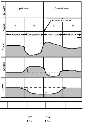
Traffic flow characteristics during a freeway incident can be characterized in terms of the four flow regions illustrated in Figure 2 Flow region A is far enough upstream of the incident so that traffic moves at normal speeds with normal density. Flow region B is thearea

located directly behind the incident where vehicles are queuing if traffic demand exceeds the restricted capacity caused by the incident. In this region, characterized by the upstream propagation of a shock wave, speeds are generally lower, and a greater vehicle density may exist. Flow region C is the region directly downstream from the incident where traffic is flowing at a metered rate, or incident flow rate, due to the restricted capacity caused by the incident. Depending on the extent of the capacity reduction, traffic density in region C can be lower than normal, while the corresponding traffic speed is generally higher than normal. Flow region D is far enough downstream from the incident such that traffic in D flows at normal density and speed, as in region A. The source of this figure is [Traffic Detector Handbook, 2006].

Figure 2. Traffic flow characteristics and direction of density and flow changes during an

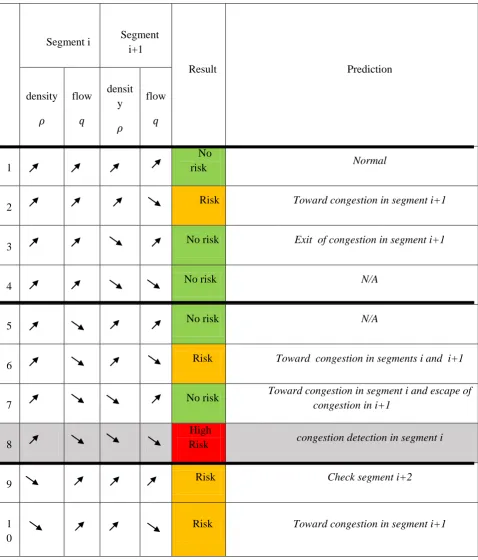
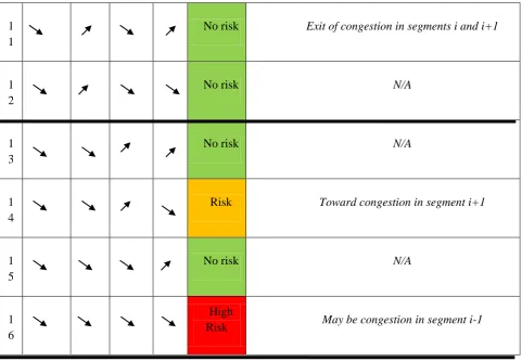
91 International Journal of Transportation Engineering, Vol.6/ No.1/ Summer 2018 By considering the density (𝜌 ) and flow

(𝑞) of 𝑖th and (𝑖 + 1)th segment, it will be16

different circumstances for trend changes of density and flow (Table 1).

Table 1. Possible density and flow change trends in two sequential segments i and i+1

Segment i Segment i+1

Result Prediction

density 𝜌

F flow

𝑞

D densit

y 𝜌

F flow

𝑞

1 1

No

risk Normal

2

2 Risk Toward congestion in segment i+1

3

3 No risk Exit of congestion in segment i+1

4

4 No risk N/A

5

5 No risk N/A

6

6 Risk Toward congestion in segments i and i+1

7

7 No risk

Toward congestion in segment i and escape of congestion in i+1

8 8

High

Risk congestion detection in segment i 9

9 Risk Check segment i+2

1 1 0

1 1 1

No risk Exit of congestion in segments i and i+1

1 1 2

No risk N/A

1 1 3

No risk N/A

1 1 4

Risk Toward congestion in segment i+1

1 1 5

No risk N/A

1 1 6

High

Risk May be congestion in segment i-1

Row 8 in Table 1 shows the situation of incident detected at segment i as it shows in Figure 2. Some other rows show different risk of congestion or abnormal traffic flows in segments iand i+1.

3.3

Direction Detection of

𝐪

and

𝛒

Trends

In predefined conditions, we collect 𝑚(𝑘) and 𝑣(𝑘)and calculate 𝑞(𝑘) and 𝜌(𝑘)from each segment. By attention to previous samples, the last 𝑛 samples of traffic flow behavior in 𝑖th

segment will be like below time series: The time series of traffic flow:

𝑞𝑖(1),𝑞𝑖(2),…,𝑞𝑖(𝑛) (1) The time series of traffic density:

𝜌𝑖(1), 𝜌𝑖(2), …, 𝜌𝑖(𝑛) (2)

And for the(𝑖 + 1)th segment:

𝑞_𝑖+1(1), 𝑞_𝑖+1(2),…, 𝑞_𝑖+1(𝑛) (3) 𝜌_𝑖+1(1), 𝜌𝑖+1(2)…, 𝜌𝑖+1(𝑛) (4)

In this condition:

𝑞_𝑖+1(𝑛) = 𝑞𝑖(1) and 𝜌𝑖+1(𝑛) = 𝜌𝑖(1)

93 International Journal of Transportation Engineering, Vol.6/ No.1/ Summer 2018 between observations at different times. The set

of autocorrelation coefficients arranged as a function of separation in time is the sample autocorrelation function, or the acf. Equation (5) can be generalized to give the autocorrelation factor between observations separated by k time steps:

𝑟_𝑘 =∑𝑛−𝑘𝑖=1(𝑥𝑖–𝑥̅)(𝑥𝑖+𝑘–𝑥̅)

∑𝑛𝑖=1(𝑥𝑖–𝑥̅)2 (5)

The quantity is called the autocorrelation coefficient at lag k. The plot of the autocorrelation function as a function of lag is also called the correlogram. If the function (5) is well-defined, its value must lie in the range [−1, 1], that 1 indicating perfect correlation and −1 indicating perfect anti-correlation. The autocorrelation at lag 3 for two time series of𝜌𝑖(𝑘)and 𝑞𝑖(𝑘)of equations1 and 2with 12 samples (every sample is the average of 5 minutes data) of the last 60 minutes for the 𝑖th

segment are: 𝑟3[𝑞𝑖(𝑘)]

=∑ [𝑞𝑖(𝑘)– 𝑞̅̅̅̅̅̅̅][𝑞𝑖(𝑘) 𝑖(𝑘 + 3)– 𝑞̅̅̅̅̅̅̅]𝑖(𝑘) 𝑇−𝑙𝑎𝑔

𝑘=1

∑12𝑘=1(𝑞_𝑖(𝑘)– 𝑞̅̅̅̅̅̅̅)𝑖(𝑘) 2

Where

𝑞̅̅̅̅̅̅̅ = 𝑖(𝑘) ₁₂1 ∑1224𝑘=1 𝑞𝑖(𝑘) (6)

And 𝑟₃[𝜌_𝑖(𝑘)]

=∑ [𝜌𝑖(𝑘)– 𝜌̅̅̅̅̅̅̅][𝜌𝑖(𝑘) 𝑖(𝑘 + 3)– 𝜌̅̅̅̅̅̅̅]𝑖(𝑘) 𝑇−𝑙𝑎𝑔

𝑘=1

∑12 (𝜌_𝑖(𝑘)– 𝜌̅̅̅̅̅̅̅)_𝑖(𝑘) 2 𝑘=1

Where 𝜌̅̅̅̅̅̅̅̅̅̅ = 𝑖(𝑘) ₁₂1 ∑1224𝑘=1 𝜌𝑖(𝑘) (7)

The results of two above equations are between 1 and -1. If it is a positive number, it means a persistent trend on changing 𝜌or𝑞, but

it does not show the positive trend or negative trend (increasing or decreasing of 𝜌 or 𝑞). If it is equal to zero, it shows a fully random changes and non-existent trend. To determine the direction of the trend, it’s enough to calculate:

[𝑞̅̅̅̅̅̅̅ − 𝑞_𝑖(𝑘) _𝑖(1)]and[𝜌̅̅̅̅̅̅̅ − 𝜌_𝑖(𝑘) _𝑖(1)] (8)

If the result is a positive number, it shows the positive trend and if the result is negative, it shows the negative trend. The same equations could be generated for 𝑟3[𝑞𝑖+1(𝑘)] and 𝑟₃[𝜌𝑖+1(𝑘)] to find any existent trend of density and flow in segment (𝑖 + 1)th. Now by applying the trend directions of density and flow of two sequential segments, 𝑖thand (𝑖 + 1)th, in the Table 1, the traffic condition or abnormality in segment 𝑖thwill be detected.

4.

Implementation

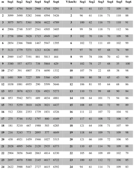
We evaluated the proposed method using different data sources of real traffic scenes from Tehran-Qom freeway, Iran. The source of data is the database of Road Maintenance and Transportation Organization (RMTO). A total of 480 minutes, which corresponds to interstate highways, are chosen for testing. The number of passed vehicle and mean speed are collected by six traffic counter every 1 minute and time period of algorithm is 24minute. Table 2 shows total number of passed vehicles and time mean speed in six segment at one time period of algorithm(T). (Table 2)

Table 2. Total number of passed vehicles and time mean speed in 6 segments at one time period of algorithm

m Seg1 Seg2 Seg3 Seg4 Seg5 Seg6 V(km/h) Seg1 Seg2 Seg3 Seg4 Seg5 Seg6 1 3087 4794 5618 2968 4744 5291 1 91 61 113 72 109 86 2 3099 3490 5282 3446 4594 5426 2 96 61 116 71 110 88 3 3075 5071 5361 3036 4622 4789 3 100 62 116 73 110 91 4 2906 2748 5197 2541 4505 3405 4 99 58 118 71 112 96 5 2758 1894 5828 1715 4949 2467 5 102 70 116 70 109 98 6 2854 2366 7068 1467 5947 1395 6 102 72 111 69 102 99

7 3121 1779 7271 1212 6126 693 7 97 70 97 68 74 99

8 2989 1167 7191 881 5813 464 8 99 78 106 70 62 99

9 3380 557 6373 738 5864 629 9 102 78 27 68 35 100

10 2747 391 4807 374 4690 1332 10 107 79 22 68 38 98

11 1481 509 7227 309 5366 4245 11 104 80 58 65 43 90

12 1038 1081 6955 290 5599 5646 12 106 81 95 64 68 86

13 853 3876 6213 326 4921 5273 13 110 73 99 68 90 84

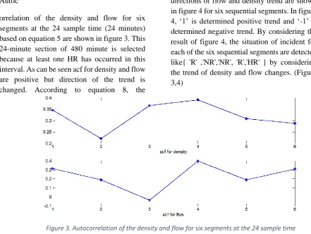
95 International Journal of Transportation Engineering, Vol.6/ No.1/ Summer 2018 Autoc

orrelation of the density and flow for six segments at the 24 sample time (24 minutes) based on equation 5 are shown in figure 3. This 24-minute section of 480 minute is selected because at least one HR has occurred in this interval. As can be seen acf for density and flow are positive but direction of the trend is changed. According to equation 8, the

directions of flow and density trend are shown in figure 4 for six sequential segments. In figure 4, ‘1’ is determined positive trend and ‘-1’ is determined negative trend. By considering the result of figure 4, the situation of incident for each of the six sequential segments are detected like{ 'R' ,'NR','NR', 'R','HR' } by considering the trend of density and flow changes. (Figure 3,4)

Figure 3. Autocorrelation of the density and flow for six segments at the 24 sample time

Data acquisition time interval (time step) (𝝉)

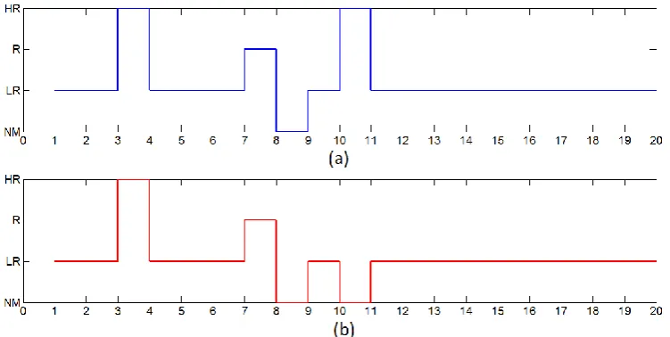
Figure 5. a) Actual b) estimated, traffic states for segment 1 over 20 time intervals of T

We have compared results of this method with the actual events in the same period of time in Tehran-Qom freeway. Figure 5(a) is the real traffic situation for segment 1 over 20 time intervals of T and figure 5(b) is the results of the proposed method. As shown in figure 5, the model has estimated correct traffic conditions for most of the intervals just for T 10 to 11. It shows %95 accuracy rates for traffic condition estimation using this

5.

Conclusion

In this paper we discussed the model of using autocorrelation of flow and density of freeway traffic to predict the short time traffic condition. After implementing proposed method using a total of 480 minutes data of real traffic scenes from Tehran-Qom freeway, Iran, autocorrelation of the density and flow for six segments at the 24 sample time (24 minutes) showed us the trend direction of changes in flow and density of traffic. According to the model definitions 3-state traffic pattern prediction implemented as No Risk (NR), Risk (R) and High risk (HR). The situation of incident for each of the six sequential segments

are detected like{'R' ,'NR','NR', 'R','HR' } in the mentioned case study by considering the trend of density and flow changes. This technique will be applicable for any other conditions. The best scenario can be designed for different conditions after adjusting and finding the optimum quantities for the parameters: normal speed, segment length, time period, time interval of data acquisition and the autocorrelation lag and the same table can be achieved .The proposed model estimated traffic condition properly with 95 percent accuracy rate.

97 International Journal of Transportation Engineering, Vol.6/ No.1/ Summer 2018

6.

References

-Abdulhai, B. and Ritchie, S. G. (1999) “Enhancing the universality and transferability of freeway incident detection using a Bayesian-based neural network”, Transportation Research Part C 7, pp. 261–280.

-Adeli, H. and Karim, A. (2000) “Fuzzy-wavelet RBFNN model for freeway incident detection”, Journal of Transportation Engineering Vol. 126, No. 6, pp. 464–471.

-Ahmed, S. A. (1983) “Stochastic processes in freeway traffic”, Traffic Engineering Control, pp.306–310.

-Aultman-Hall, L., Hall, F.L., Shi, Y. and Lyall, B. (1991) “A catastrophe theory approach to freeway incident detection”, Proceedings of the Second International Conference on Applications of Advanced Technologies in Transportation Engineering, The American Society of Civil Engineers, New York, NY, pp. 373–377.

-Chang, E. C.-P. and Wang, S.-H. (1995) “Improved freeway incident detection using fuzzy set theory”, Transportation Research Record Vol. 1453, 75–82.

-Cook, A. R. and Cleveland, D. E. (1974) “Detection of freeway capacity-reducing incidents by traffic-stream measurements”, Transportation Research Record, Vol. 495, pp.1– 11.

-Daganzo, C. (1995) “The cell transmission model, Part II: Network traffic” Transportation Research,Part B, Vol. 29, No. 2, pp.79–93.

-Dudek, C. L. and Messer, C. J. (1974) “Incident detection on urban freeways” Transportation Research Record, Vol.495, pp. 12–24.

-Golob T. F., Will, Rocker and Yannis, Pavlis (2008) “ Probabilistic models of freeway safety performance using traffic flow data as predictors”, Safety Science, Vol.46 (2008) pp.1306-1333

-Hoogendoorn, S. P. and Bovy, P. H. L. (2001) “State of the art of vehicular traffic flow modelling“, Jornal of Systems and Control engineering, Vol.215(4)

-Hsiao, C.-H., Lin, C.-T. and Cassidy, M. (1994) “Application of fuzzy logic and neural networks to automatically detect freeway traffic incidents” Journal of Transportation Engineering Vol.120 (5), pp.753–772.

-Ishak, S. and Al-Deek, H. (1999) “Performance of automatic ANN-based incident detection on freeways” Journal of Transportation Engineering, pp.281–290.

-Kerner, B. S. (2013) “Criticism of generally accepted fundamentals and methodologies of traffic and transportation theory”, A brief review Physic A: Statistical Mechanics and its ApplicationsVol. 392 (21), pp. 5261-5282.

-Lin, W.-H. (1995) “Incident detection with data from loop surveillance systems: the role of wave analysis”, Dissertation, Institute of Transportation Studies, University of California at Berkeley.

-Payne, H. J. and Tignor, S. C. (1978) “Freeway incident detection algorithms based on decision trees with states”, Transportation Research Record, Vol. 682, pp.30–37.

-Porikli, F. and Li, X. (2004) “Traffic congestion estimation using HMM models without vehicle tracking”, Mitsubishi Electronic Reserch Labratories

-Qiu, T.Z., Lu, X., Chow, A. H. F. and Shladover, S. E. (2010) “Estimation of freeway traffic density with loop detector and prob vehicle data“, Transportation Research Record, Jornal of Transportation Research Board, No. 2178, pp. 21-29.

-Stephanedes, Y. J. and Chassiakos, A. P. (1993) “Application of filtering techniques for incident detection”, Journal of Transportation Engineering, Vol. 119, No. 1, pp.13–26.

-Torfehnejad, H. (2011) “A practical dynamic speed limit control method using real-time traffic counting systems“, 18th ITS World Congress, 16-20 October, Orlando Florida, USA

-Torfehnejad, H. and Adamnejad, Sh. (2014) “A practical symple technique to detect abnormal traffic flow in freeway“, 21th ITS World Congress, 7-11September, Detroit, USA

-U.S. Department of Transportation. Federal Highway Administration (2006) “Traffic detector handbook“, Third edition- Volume 1

-Whitson, R. H., Burr, J. H., Drew, D. R. and McCasland, W. R. (1969) “Real-time evaluation of freeway quality of traffic service” Highway Research Record, Vol. 289, pp.38–50.

-Willsky A. S., Chow E.Y.,. Gershwin, S. B, Greene, C. S., Houpt, P. K. and Kurkjian, A. L. (1980) “Dynamic model-based techniques for the detection of incidents on freeways“ , IEEE Transactions on automatic control, Vol. AC-25, No.3