https://doi.org/10.5194/essd-9-697-2017 © Author(s) 2017. This work is distributed under the Creative Commons Attribution 3.0 License.
Global fire emissions estimates during 1997–2016
Guido R. van der Werf1, James T. Randerson2, Louis Giglio3, Thijs T. van Leeuwen4,a, Yang Chen2, Brendan M. Rogers5, Mingquan Mu2, Margreet J. E. van Marle1,b, Douglas C. Morton6,
G. James Collatz6, Robert J. Yokelson7, and Prasad S. Kasibhatla8
1Faculty of Earth and Life Sciences, Vrije Universiteit Amsterdam, 1081 HV Amsterdam, the Netherlands 2Department of Earth System Science, University of California, Irvine, CA 92697, USA
3Department of Geographical Sciences, University of Maryland, MD 20742, USA 4SRON Netherlands Institute for Space Research, 3584 CA Utrecht, the Netherlands
5Woods Hole Research Center, Falmouth, MA 02540, USA
6Biospheric Sciences Laboratory, NASA Goddard Space Flight Center, Greenbelt, MD 20771, USA 7Department of Chemistry, University of Montana, Missoula, MT 59812, USA
8Nicholas School of the Environment, Duke University, Durham, NC 27708, USA anow at: VanderSat BV, 2011 VK, Haarlem, the Netherlands
bnow at: Deltares, 2629 HV, Delft, the Netherlands
Correspondence to:Guido R. van der Werf ([email protected])
Received: 9 December 2016 – Discussion started: 12 January 2017 Revised: 6 July 2017 – Accepted: 18 July 2017 – Published: 12 September 2017
1 Introduction
Fires have occurred naturally since the rise of vascular plants on land over 400 million years ago (Scott and Glasspool, 2006), shaping biomes and influencing climate through mod-ulation of the carbon cycle and emissions of greenhouse gases and aerosols (Edwards et al., 2010; Langmann et al., 2009; van Langevelde et al., 2003). During the An-thropocene, humans have become an increasingly important driver of fire occurrence (Bowman et al., 2011). Human ac-tivity has enhanced fire acac-tivity in locations such as defor-estation zones, while fire suppression and conversion of fire-prone landscapes such as savannas to agriculture in Africa, or of fire-maintained open lands to closed-canopy forests in the eastern US has generally decreased fire activity (Andela and van der Werf, 2014; Bowman et al., 2009; Nowacki and Abrams, 2008). To study how climate influences fires at the global scale and, in turn, how fires influence the carbon cy-cle, air quality, and climate we have developed the Global Fire Emissions Database (GFED).
The scientific community has used past releases of GFED for over a decade. GFED has been used by atmospheric and biogeochemical modeling groups as an input dataset to study the impact of fires on biogeochemical cycles (Chen et al., 2010; Schwietzke et al., 2016), atmospheric chemistry (Aouizerats et al., 2015; Castellanos et al., 2014), and hu-man health (Johnston et al., 2012; Marlier et al., 2013), in assessment reports of the Intergovernmental Panel on Cli-mate Change (IPCC) to estiCli-mate the role of fire and de-forestation in biogeochemical cycles (Ciais et al., 2013), in the National Oceanic and Atmospheric Administration (NOAA’s) CarbonTracker system (Peters et al., 2007), and in annual updates of the Global Carbon Project (Le Queré et al., 2015). GFED also serves as a benchmark for optimiz-ing fire modules in dynamic global vegetation and Earth sys-tem models (Hantson et al., 2016), and for fire emissions es-timates derived from fire radiative power (FRP), including the Global Fire Assimilation System (Kaiser et al., 2012). Finally, burned area from GFED has provided a means for building early warning systems of fire season severity (Chen et al., 2016).
The first version of GFED was released in 2004 and has since undergone several revisions as improved burned area estimates became available. GFED2 was released after Giglio et al. (2006) improved on the mapping of burned area from active fire data. GFED3 was released when this con-version was no longer necessary because almost all burned area in the Moderate Resolution Imaging Spectroradiome-ter (MODIS) era had been mapped (Giglio et al., 2010), and the current version follows further improvements in the burned area algorithm (Giglio et al., 2013). Satellite burned area is the most important input dataset regulating the spa-tial and temporal pattern of emissions following the Seiler
and Crutzen (1980) approach, and is complemented in GFED by a biogeochemical modeling framework that provides esti-mates of biomass in various carbon “pools” including leaves, grasses, stems, coarse woody debris, and litter. These pools are combusted to different degrees during a fire depending on pool-specific parameters and environmental conditions that influence fuel moisture and the simulated burn depth in or-ganic soils of boreal forests and peatlands.
Over the past decade, a parallel line of research has made considerable progress in estimating emissions using satel-lite observations of FRP. When continuous observations are available or the FRP diurnal cycle can be modeled, FRP can be integrated over time, yielding fire radiative energy (FRE). FRE is directly related to fire emissions (Wooster, 2002), and approaches using FRP observations can provide emis-sions estimates in near-real time (Darmenov and da Silva, 2015; Kaiser et al., 2012). Despite progress (Ichoku and El-lison, 2014; Schroeder et al., 2014a), there is still substan-tial uncertainty and some of these FRE approaches apply a scaling factor to match GFED. Comparisons between the “classical” burned area approach and the FRP approach, or approaches based on active fire detections in general, have indicated there is considerable variability in the amount of burned area associated with an individual active fire detec-tion, and thus the two approaches do not always align (Giglio et al., 2006; Randerson et al., 2012). In general, direct map-ping of burned area excels when fires are large, but has diffi-culty in detecting smaller fires, for example, in croplands and in other areas where many fires have a size below the 21 ha of an individual 500 m MODIS pixel. Combining both burned area and active fire data, Randerson et al. (2012) provided ev-idence that the total area burned by these relatively small fires could be substantial at the global scale. Therefore, emission estimates based solely on active fires, including the Fire IN-ventory from NCAR (Wiedinmyer et al., 2011), may better capture spatial and temporal variability in regions with many small fires than emission estimates based solely on burned area (Reddington et al., 2016). However, approaches based solely on active fires often do not account for spatial and tem-poral variability in the amount of burned area per active fire detection or variability in fuel consumption within biomes.
and is the product of fuel load and combustion completeness. Besides these two main improvements over earlier versions, we made a number of additional modifications including up-dated input datasets, the use of satellite-derived estimates of parameters governing fuel consumption and tree mortality in the boreal region (Rogers et al., 2015), and application of a new emission factor methodology that separates temperate and boreal forest ecosystems (Akagi et al., 2011). In Sect. 2 we provide more detail on these input datasets, followed by a description of the modeling framework in Sect. 3. Results are given in Sect. 4 followed by a discussion in Sect. 5 that in-cludes a description of the main differences with GFED3 and an assessment of the primary sources of uncertainty in esti-mating fire emissions. In the conclusions (Sect. 6) we sum-marize the main points of our analysis and describe several important directions for future work.
2 Input datasets
Our version of the Carnegie–Ames–Stanford Approach (CASA) model described in Sect. 3 requires input datasets on vegetation characteristics, meteorology, and fire param-eters. Most of these datasets are somewhat different from those used in previous versions of GFED, in part from a need for shorter latency in our updates. We re-gridded all of the input datasets to 0.25◦spatial resolution and a monthly tem-poral resolution. We took additional steps to create estimates of fire dynamics on daily and 3-hourly time steps.
2.1 Vegetation characteristics
In CASA, the fraction of absorbed photosynthetically active radiation (fAPAR) is used to estimate net primary production (NPP), fractional tree cover (FTC) is used in the allocation of NPP between living carbon pools, and land cover (LC) is used to set turnover rates for stems and leaves, applying emission factors, and for categorizing fire carbon emissions into various fire types.
We calculated fAPAR based on the Global Inventory Mod-eling and Mapping Studies (GIMMS) normalized difference vegetation index (NDVI) version 3g (Pinzon and Tucker, 2014) and relations established by Los et al. (2000). This dataset is derived from the Advanced Very High Resolution Radiometer (AVHRR) sensor flying on board several satel-lites. We capped fAPAR at 0.95, corresponding to an NDVI value of 0.9. Data were not available for several remote is-lands, including Hawaii and Fiji, and we do not report emis-sions for these locations.
FTC was derived by aggregating the annual MODIS MOD44B vegetation continuous fields (250 m, V051; Hansen et al., 2005) to 0.25◦. In order to provide consis-tency over the full time period, we used the last year available (2013) and increased FTC in prior years using the fire-driven deforestation rates. These fire-driven deforestation rates were based on the amount of burned area within tropical forests at
an annual time step. We used land cover maps from the an-nual MODIS MCD12C1 land cover type product and Univer-sity of Maryland (UMD) classification scheme (Friedl et al., 2010). The climate modeling grid (CMG, 0.05◦) dataset was resampled to 0.25◦ based on the most abundant land cover type. This dataset was available for 2001–2012; data from 2001 were applied to earlier years in the time series, and 2012 land cover data were used for years after 2012.
2.2 Meteorological datasets
We now use air temperature (t2m), soil moisture (swvl), and solar radiation (ssrd) from the ERA-Interim dataset (Dee et al., 2011) produced by the European Centre for Medium-Range Weather Forecasts (ECMWF). We calculated the monthly mean for all datasets and regridded the 0.75◦dataset to our 0.25◦resolution without interpolation.
These datasets are somewhat different from inputs for earlier GFED versions but are now internally consis-tent. Interannual and seasonal variability was relatively similar to datasets previously used in GFED, and these variations have the largest impact on our calculations. The use of soil moisture is new; previously, we used a bucket model based on rainfall and potential evapora-tion to calculate the wetness of soils, a key input dataset for calculating heterotrophic respiration (Rh) rates and
combustion completeness (see Sect. 3). Soil moisture is now transformed to a soil moisture index (SMI) based on soil-type-specific permanent wilting point (PWP) and field capacity (FC) values as described in http://www.ecmwf. int/en/forecasts/documentation-and-support/evolution-ifs/ cycles/change-soil-hydrology-scheme-ifs-cycle and is capped at 1. This was done for all four different soil layers (0–7, 8–28, 29–100, 101–255 cm). The SMI for the 0–7 cm layer replaced the scalar used previously for combustion completeness. The average SMI of the top two layers was used to down-regulate NPP in herbaceous vegetation in the light use efficiency model when moisture was limiting, whereas the average of the top four layers was used for NPP in woody vegetation. The average SMI for the upper two layers was also used to represent the influence of soil moisture on the abiotic scalar regulating rates ofRh. Finally,
the average SMI of all layers was used in the allocation of assimilated carbon to above- and belowground pools (see Sect. 3).
2.3 Fire processes
burned area data for which a more detailed description is de-scribed in Giglio et al. (2013). In Sect. 2.3.2 we then explain how the small fire burned area estimates for the MODIS era were derived based on Randerson et al. (2012). This is the GFED4s burned area time series and complemented with other sensors to compute the full 1997–2016 time period dataset (Sect. 2.3.3).
2.3.1 Burned area from MODIS
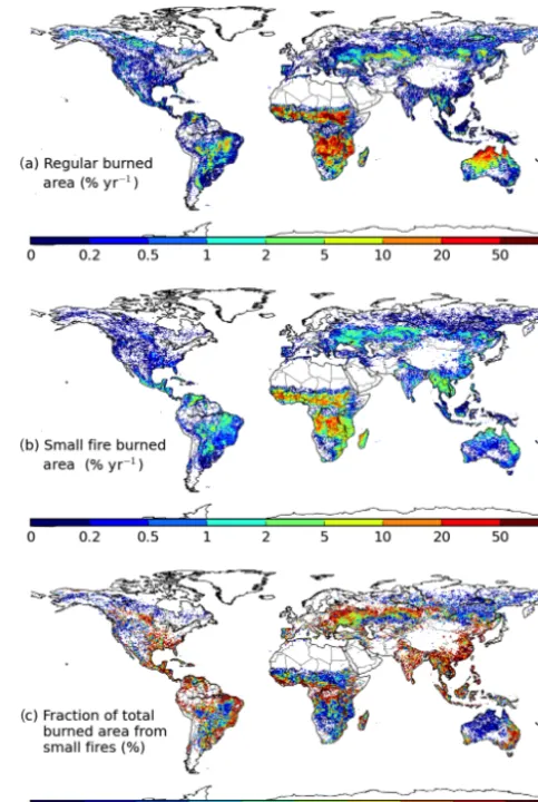
For the MODIS era we used the MODIS Collection 5.1 MCD64A1 burned area product (Giglio et al., 2013). Compared with Collection 5 and earlier versions of the MCD64A1, the Collection 5.1 product reduces the uninten-tional removal of small burns and eliminates some systematic omission errors (Giglio et al., 2013). The MCD64A1 prod-uct maps daily burned area at 500 m spatial resolution; these data are then aggregated to a 0.25◦grid (both monthly and daily) to produce the MODIS-era GFED4 burned area prod-uct (Fig. 1a).
2.3.2 Small fire burned area during the MODIS era
In the MODIS era, we combined 500 m burned area (see above), 1 km thermal anomalies (active fires) from Terra and Aqua MODIS, and 500 m surface reflectance observations to statistically estimate burned area associated with small fires, BAsf, in each 0.25◦grid cell (i), month (t), and aggregated
vegetation type (v):
BAsf(i, t, v)=FCout(i, t, v)×αr, s, v, y ×γr, s, v, y, (1)
where FCout is the number of active fire pixels outside of
the perimeter of the MCD64A1 burned area,αis a ratio of burned area to active fires within MCD64A1 burned areas, andγ is a correction factor derived by comparing difference normalized burned area (dNBR) of active fires observed out-side (dNBRout) and inside (dNBRin) of MCD64A1 burned
areas with unburned control areas (dNBRcontrol; see Eq. 4 of
Randerson et al., 2012).αandγscalars were estimated each year (y), as a function of region (r), seasonal interval (s), and aggregated vegetation type (v). Our method was similar to that described in Randerson et al. (2012), but with several important modifications to each of the three factors on the right-hand side of Eq. (1) as described below.
First, we used the MCD64A1 product from Collection 5.1, replacing Collection 5 that was used in Randerson et al. (2012). Second, instead of using a single source of level 3 composited thermal anomaly/fire product from Terra (MOD14A1), here we used individual active fire detec-tions from both Terra and Aqua. Third, to improve geolo-cation accuracies, we used the MODIS fire logeolo-cation product (MCD14ML) instead of the gridded composite fire product (MOD14A1). To further reduce geolocation uncertainties, we only retained active fire detections with small or moderate
Figure 1.Average burned area over 2003–2016 from(a)MODIS surface reflectance imagery (MCD64A1) and(b)small fire burned area. Panel(c)shows the small fire percentage of total burned area.
0.00 0.08 0.16
(a) NHAF
Original (b) CEASOriginal
-0.5 0 0.5 1
dNBR 0.00
0.08 0.16
Normalized pdf
(c) NHAF Modified
-0.5 0 0.5 1
dNBR (d) CEAS Modified
Figure 2. The distribution of difference normalized burn ra-tio (dNBR) for active fires detected within burned areas from MCD64A1 (red), outside of burned areas (orange), and for control areas (blue) within Northern Hemisphere Africa (NHAF) and Cen-tral Asia (CEAS). The distributions, generated using observations in 2001–2012, were constructed during the peak fire month for each region. The improved approach (see Sect. 2.3.2 for details) com-pressed the distributions in unburned control areas and increased the separation between the three categories.
a stricter criterion than in Randerson et al. (2012) that in-creases dNBRinand its separation from dNBRoutand other
areas used as controls (Fig. 2).
It was not possible to apply the same constraint in the cal-culation of dNBRout, so this adjustment usually had the effect
of loweringγ. We note that dNBRoutin particular is strongly
affected by resampling error; thus, the individual γ correc-tion factors are in turn also influenced by resampling error. The net effect is to limit the range of values that may be at-tained byγ, in a sense leaving an “imprint” of resampling error on the resulting small fire burned area estimates. This imprint is an unavoidable outcome of using relatively coarse 1 km and 500 m gridded time series data to track small, sub-pixel fires. At the same time, we raised the filtering standard for control pixels (Eq. 4 of Randerson et al., 2012) so that pixels within a 1 km buffer area of active fire detections by either Terra or Aqua MODIS were excluded in the calcula-tion of dNBR for non-burning areas (dNBRcontrol). During
the regional aggregation of dNBR, we excluded 500 m pix-els that were marked as “water” by MODIS land cover type product (MCD12Q1).
During the time both Terra and Aqua fire detections were available (January 2003–December 2016), we calcu-lated BAsf separately for Terra (MOD) and Aqua (MYD).
BAsf was then estimated as the arithmetic mean of the two
estimates. A climatological ratio of BAsf−MYD/BAsf−MOD
was used to estimate BAsf−MYD during periods when Aqua
MODIS observations were not available (August 2000–
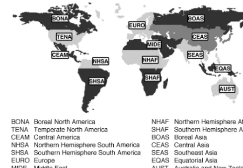
Figure 3.Map of the 14 regions used in this study, after Giglio et al. (2006) and van der Werf et al. (2006).
December 2002). The final GFED4s burned area during the MODIS era was the sum of GFED4 burned area (Sect. 2.3.1; Fig. 1a) and burned area from small fires (BAsf, Fig. 1b).
As expected, burned area from small fires is more preva-lent in areas with extensive agriculture and in other human-dominated landscapes (Fig. 1c).
2.3.3 Estimating burned area prior to the MODIS era (1997–2000) for GFED4s
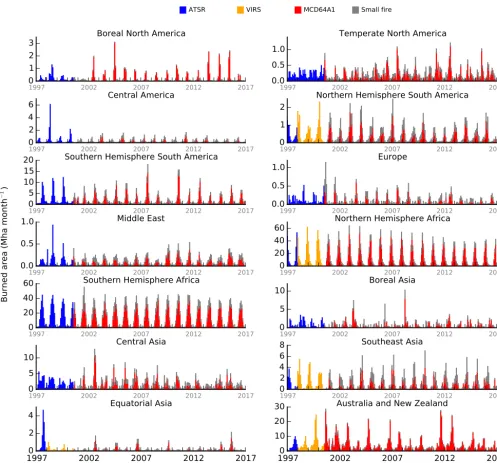
For the pre-MODIS era, we used monthly active fire data from the Visible and Infrared Scanner (VIRS) aboard the Tropical Rainfall Measuring Mission (TRMM) or the Along Track Scanning Radiometers (ATSR) on board multiple plat-forms to estimate burned area. Two steps of optimization were used to derive total burned area, starting with the GFED4s product described above. The first step was to de-velop a relationship between aggregated active fires (from VIRS or ATSR) and burned area during the MODIS era in each GFED region, with the aim of using this relationship to estimate regional burned area during 1997–2000. The second step involved distributing the aggregated burned area within each region to individual 0.25◦grid cells.
data in all other regions (Fig. 4). Prior to 1998, when VIRS data were not available, regressions based on ATSR were used. If the ATSR or VIRS active fires for any given month were outside the dynamic range of active fires during the MODIS era, we instead used linear regression derived from all of the monthly data during the MODIS era for that region. After quantifying the sum of burned area within each re-gion, we distributed it among 0.25◦grid cells using the fol-lowing approach. While active fires from ATSR or VIRS pro-vide some indication about the temporal dynamics of fire in a region, the active fire approach tends to underestimate burn-ing in savannas and other areas with herbaceous fuels. To as-sess how well active fires captured regional spatial patterns, we estimated the spatial correlation between active fires and burned area in each GFED region during the MODIS era. Higher correlations from these analyses indicated better agreement between the spatial distribution of ATSR/VIRS active fires and GFED4s burned area. Since we found the correlation coefficients varied seasonally, a mean monthly (m) set of spatial correlation coefficients (SC) was derived to determine the level of representation of burned area by ATSR/VIRS active fires. The spatial distribution function of burning was based on a linear combination of climatological distribution of burned area (cl) and the distribution of active fires (FC):
BApre−MODIS(i, t)=BArs(r, t)×[SDFFC(r, i, t)×SC (r, m)
+SDFcl(r, i, t)×(1−SC (r, m)) ], (2)
where SDFFC and SDFcl are unitless spatial distribution
functions that each sum to 1 in each GFED region and were derived from active fire detections or the monthly climatol-ogy of burned area during the MODIS era from GFED4s, and BArs is the regional (r) sum of burned area for that month
and region derived from the regressions between GFED4s and ATSR or VIRS active fires described above. In temper-ate and high-latitude regions, where the spatial correlation between active fires and burned area is relatively high, the equation primarily uses information from the pre-MODIS ac-tive fires to assign the spatial distribution of burned area. In regions where the spatial correlation between active fires and burned area is relatively low, the equation relies more on the climatological burned area pattern from the MODIS era. For consistency with the previous step, the source of the active fires for generating the SDF was the same as active fires used to generate the regional sum of burned area in each region. The contribution of ATSR, VIRS, MCD64A1, and BAsf to
the total burned area is shown in Fig. 4 for the GFED4s time series.
2.3.4 Combustion completeness and fire-induced mortality in boreal forests
Despite relatively similar environmental conditions and veg-etation attributes, the boreal regions in North America and
Eurasia exhibit significantly different patterns of fire sever-ity (Wooster and Zhang, 2004). This was shown to primarily be a function of divergent plant traits for the dominant tree species in each continent (Rogers et al., 2015). Species in North America tend to promote crown fires with higher lev-els of combustion completeness of the canopy and tree mor-tality compared to lower-severity surface fires in Eurasia. As with other global fire models, GFED3 did not capture these differences due to biome-wide parameterizations.
To address the large-scale differences in boreal fire effects, we integrated satellite-based metrics of severity from Rogers et al. (2015) including immediate tree mortality and an index of vegetation destruction. These were initially calculated at 1 km and 500 m resolutions, respectively, and aggregated to 1◦, but here rescaled to our 0.25◦grid without interpolation. Vegetation destruction was derived from three MODIS-based metrics that provide information on immediate fire-induced losses of green vegetation, reduction in canopy and soil wa-ter, and landscape charring. These included dNBR, decreases in NDVI, and increases in summer land surface temperature (LST). The original vegetation destruction product used LST from Aqua and was available from 2003 to 2012. We ex-tended it here to 2001 and 2002 using multiple linear regres-sion relationships based on Terra LST, dNBR, and changes in NDVI at 1◦(r2=0.95 for North America, 0.96 for northwest Eurasia, 0.95 for northeast Eurasia, and 0.91 for southern Eurasia). Immediate tree mortality was based on decreases in tree cover and increases in spring albedo 1 year after a fire, and was provided for fires between 2001 and 2009. For both products, grid-cell-specific averages were used in years not covered, and grid cells without valid values were assigned regional burned-area-weighted means. On average, vegeta-tion destrucvegeta-tion was 36 % lower and fire-induced tree mor-tality was 42 % lower in boreal Eurasia compared to boreal North America. More details on model integration are given in Sect. 3.1, and more information on these products can be found in Rogers et al. (2015).
3 Modeling framework and modifications
ATSR VIRS MCD64A1 Small fire
1997 2002 2007 2012 2017
0
1
2
3
Boreal North America
1997 2002 2007 2012 2017
0.0
0.5
1.0
Temperate North America
1997 2002 2007 2012 2017
0
2
4
6
Central America
1997 2002 2007 2012 2017
0
1
2
Northern Hemisphere South America
1997 2002 2007 2012 2017
0
5
10
15
20
Southern Hemisphere South America
1997 2002 2007 2012 2017
0.0
0.5
1.0
Europe
1997 2002 2007 2012 2017
0.0
0.5
1.0
Bu
rn
ed
ar
ea
(M
ha
m
on
th
−
1
)
Middle East
1997 2002 2007 2012 2017
0
20
40
60
Northern Hemisphere Africa
1997 2002 2007 2012 2017
0
20
40
60
Southern Hemisphere Africa
1997 2002 2007 2012 2017
0
5
10
Boreal Asia
1997 2002 2007 2012 2017
0
5
10
Central Asia
1997 2002 2007 2012 2017
0
2
4
6
8
Southeast Asia
1997
2002
2007
2012
2017
Year
0
2
4
Equatorial Asia
1997
2002
2007
2012
2017
Year
0
10
20
30
Australia and New Zealand
Figure 4.Regional time series (1997–2016) of GFED4s monthly burned area. The different colors indicate the contribution from each of the different data sources and methodologies (ATSR, TRMM-VIRS, 500 m MCD64A1, and small fires) used to produce the entire dataset.
3.1 CASA-GFED framework
When CASA was developed it computed carbon fluxes as the difference between NPP andRh. Both are still calculated for
each month and each 0.25◦grid cell. NPP is based on a light use efficiency model (Field et al., 1995) and is distributed over various live biomass “pools” (leaves, stems, roots) ac-cording to satellite-derived fractional tree cover maps. In forests we allocate NPP to all three live biomass pools, and in grasslands to leaves and roots, accounting for variability in allocation due to gradients in mean annual precipitation as in GFED3. The carbon in these pools is subsequently delivered
to nine litter pools at the surface and in the soil with turnover rates set for each pool depending on moisture conditions and temperature.
0 2 4 6 8 10 12 14 16
Measured standing biomass (kg C m
−2)
0
2
4
6
8
10
12
14
16
Mo
de
led
st
an
din
g
bio
m
as
s (
kg
C
m
−
2
)
100
1000
10 000
Number of grid cells
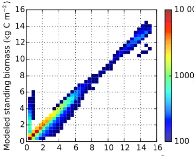
Figure 5.Comparison of modeled standing biomass with the com-pilation from Avitabile et al. (2016) and Santoro et al. (2015). Bins with fewer than 100 grid cells are excluded.
of slowly decomposing soil pools were adjusted in GFED4 to better match measured values reported for 0–30 and 30– 100 cm (Batjes, 2016).
In GFED1 we added fire, herbivory, and grazing as addi-tional carbon loss pathways besides Rh. Fires transfer
car-bon to the atmosphere and between the different pools de-pending on the burned fraction of the grid cell, combustion completeness, fire-induced mortality rates, and information on whether belowground carbon pools are susceptible to fire or not.
Combustion completeness (CC) is treated similarly in GFED4 as in our previous work with set minimum and max-imum values; see Table 1 in van der Werf et al. (2010). We scaled CC using the soil moisture index (SMI) of the top 7 cm such that the 5th and 95th percentiles corresponded with the minimum and maximum values. Fire-induced tree mortality was set to 2 % for low tree cover regions (mainly savannas and agriculture) and 50 % for forests in general but modified in tropical forests based on fire persistence as in GFED3, and in boreal regions according to satellite derived proxy datasets (Sect. 2.3.4). More specifically, in boreal forests we used the satellite-derived instantaneous tree mortality to represent fire-induced tree mortality. In addition, we did not use the CC scaling by SMI for the aboveground wood in the boreal region but used the satellite-derived vegetation destruction scalar for this. The combustion completeness of the wood pool ranged between the set minimum and maximum values (0.2 and 0.4, respectively), and linearly depended on the veg-etation destruction scalar instead of SMI.
3.2 Modifying the burned fraction to account for sub-grid-scale heterogeneity in fuels
In our previous model setup, fires lowered the fuel load in each grid cell depending on burned area, combustion com-pleteness, and fire-induced mortality rates. This was done
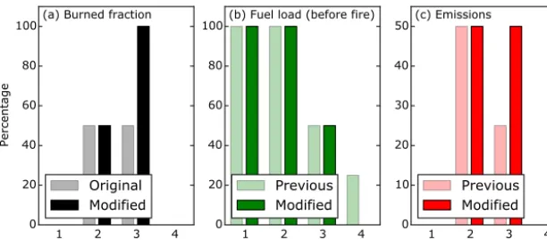
uniformly in the grid cell, not accounting for the fact that fires only lower fuel in the fraction of the grid cell that actually burned. This may have led to an underestimation of emis-sions in frequently burning regions, especially towards the end of the fire season. For example, in a grassland grid cell that burns in two consecutive months, each with 0.5 burned fraction, modeled fuel loads in the second month are half those of the first month if combustion completeness is set at 100 % (Fig. 6). In reality, the fuel load in that grid cell in the second month should be similar to that in the first month for the part that had not burned, and depleted for the part that had burned. To compensate for this effect we now calculate themodified burned fractionof the grid cell as
MBF(it)=BA(i, t)
A(i)
1−
Pt−1 t−4BA(i, t)
A(i) !
, (3)
where MBF is the modified fraction of the grid cell that burns, BA is the burned area, andAis the area of the grid cell at location (i). In our hypothetical example from above MBF now becomes 1 in the second month according to Eq. (3), thus generating similar emissions in the 2 months that each burn the same area (Fig. 6). When cumulative burned area over a fire season exceeds the grid cell area this approach yields negative values towards the end of the season; if this occurs these values are replaced by the burned area divided by the grid cell area. Because we only take into account the burned area from the actual month and the three preceding months, grid cells with two burning seasons are probably not impacted because they are usually separated in time by more than 3–4 months. Our approach does not influence the burned area datasets but only the way it is used in the conversion of burned area to emissions.
3.3 Fuel consumption optimization
Emissions are derived from the multiplication of burned area and fuel consumption per unit burned area, the latter being the product of fuel loads per unit area and combustion com-pleteness. Van Leeuwen et al. (2014) summarized the peer-reviewed literature on fuel consumption rates consisting of 76 studies and covering 121 unique measurement locations. In addition to the fuel consumption measurement, we also in-cluded the fuel load measurements mostly in savannas from Scholes et al. (2011) and assumed a combustion complete-ness of 0.9 for these fuel measurements to calculate fuel con-sumption. This latter set of 95 measurements were mostly confined to South Africa, Botswana, and Zambia.
0 20 40 60 80 100
Percentage
(a) Burned fraction
1 2 3 4
Original Modified
0 20 40 60 80
100(b) Fuel load (before fire)
1 2 3 4
Month
Previous Modified
0 10 20 30 40
50(c) Emissions
1 2 3 4
Previous Modified
Figure 6.Burned area, fuel load, and emissions for a hypothetical grid cell where 50 % of the area burns in month 2 and 50 % in month 3, and assuming a combustion completeness of 100 %. “Previous” refers to our previous work in GFED3 and before where no adjustments were made in the conversion of burned area to the fraction of fuel load that is combusted; “modified” refers to the current approach (GFED4 and GFED4s), where we treat the burned fraction as the fraction of the total remaining fuel in the grid cell that is combusted using Eq. (3).
Table 1.Emission factors for different fire types, in g specie per kg dry matter burned. Emission factors for other species, uncertainties, and source information is provided in http://www.geo.vu.nl/~gwerf/GFED/GFED4/ancill/GFED4_Emission_Factors.xlsx. Dry matter carbon content (DMCC) was derived from the carbonaceous species and used to convert carbon to dry matter.
Specie Savanna Boreal Temperate Tropical Peat Agriculture Mean emissions
forest forest forest (Tg yr−1)
CO2 1686 1489 1647 1643 1703 1585 7320
CO 63 127 88 93 210 102 357
CH4 1.94 5.96 3.36 5.07 20.8 5.82 16.1
NMHC 3.4 8.4 8.4 1.7 1.7 9.9 17.8
H2 1.7 2.03 2.03 3.36 3.36 2.59 9.31
NOx(as NO) 3.90 0.90 1.92 2.55 1.00 3.11 14.60
N2O 0.20 0.41 0.16 0.20 0.20 0.10 0.93
PM2.5 7.2 15.3 12.9 9.1 9.1 6.3 36.6
TPM 8.5 17.6 17.6 13.0 13.0 12.4 46.6
TPC (OC+BC) 3.00 10.10 10.10 5.24 6.06 3.05 18.4
OC 2.62 9.60 9.60 4.71 6.02 2.30 16.6
BC 0.37 0.50 0.50 0.52 0.04 0.75 1.86
SO2 0.48 1.10 1.10 0.40 0.40 0.40 2.32
NH3 0.52 2.72 0.84 1.33 1.33 2.17 4.22
DMCC (%) 48.83 46.50 48.94 49.18 57.01 48.04 –
but also within biomes and between separate fuel classes. The overall spatial representativeness of the fuel consump-tion field measurements is reasonable for most fiprone re-gions. However, several important regions from a fire emis-sions perspective – including Southeast Asia and Central Africa – are under-represented. For this study we used ver-sion 1 of the fuel consumption database available from http: //www.geo.vu.nl/~gwerf/FC/.
3.4 Emission factors
Emission factors are used to convert dry matter burned into emissions of trace gases and aerosols. These were assigned in GFED3 based on the compilation of Andreae and Mer-let (2001) with annual updates. A new compilation was
Jun Jul Aug Sep Oct 0
5 10 15 20
Monthly
Emissions
(g
C
m
−
2 d
ay
−
1)
GFED3
Jun Jul Aug Sep Oct
0 10 20 30 40 50 60
Daily
Emissions
(g
C
m
−
2 d
ay
−
1)
Jun Jul Aug Sep Oct
Month 0
50 100 150 200
3-hourly
Emissions
(g
C
m
−
2 d
ay
−
1)
Jun Jul Aug Sep Oct
0 5 10 15 20
Monthly
GFED4s
Jun Jul Aug Sep Oct
0 10 20 30 40 50 60
Daily
Jun Jul Aug Sep Oct
Month 0
50 100 150 200
3-hourly
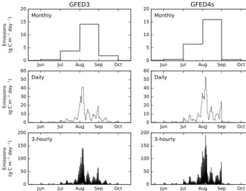
Figure 7.Comparison of monthly (top panels), and disaggregated daily (middle) and 3-hourly (bottom) emissions from GFED3 (left-hand side) and GFED4s (right-hand side) for an example grid cell in South America (11.75◦S, 51.75◦W).
http://bai.acom.ucar.edu/Data/fire/ and will be incorporated into future GFED versions.
3.5 Redistributing monthly emissions on daily and 3-hourly timescales
We made several improvements to the approach described by Mu et al. (2011) for redistributing monthly emissions to daily and 3-hourly time steps in each 0.25◦ grid cell. This set of higher temporal resolution emissions was created only for the period of 2003 to the present because of increased MODIS active fire data availability after the launch of Aqua. To estimate the daily distribution of emissions, we used two sources of information: active fires from MCD14ML and the day of burning reported in the MCD64A1 burned area product. In tropical regions between 25◦N and 25◦S, we weighted the information content from these two sources equally in grid cells for which both data streams were avail-able. In GFED3, the day of burning was not available for use as a constraint on daily variability. In the extra-tropics (poleward of 25◦N and 25◦S) we solely used active fires to distribute the daily pattern of emissions. In these regions, gaps between successive overpasses of Aqua and Terra are smaller, and active fires have been shown to be moderately effective in capturing daily variations in fire spread rates (Veraverbeke et al., 2014). We removed persistent active fire locations associated with volcanoes, gas flaring, and many
other non-fire sources, using a more recent static hotspot database (Randerson et al., 2012). A simple 3-day center mean smoothing filter was applied in tropical regions to ad-just for gaps in MODIS coverage, following Mu et al. (2011). We created a climatological diurnal cycle of burning in each region and for different aggregated vegetation types to redistribute daily emissions on a 3 h time step. The ap-proach is similar to the one described in Mu et al. (2011), and uses active fire data derived from full hemispheric scans of GOES-11 (west) and GOES-12 (east) observations dur-ing 2007–2009 with version 6.0 of the WF_ABBA algorithm (Prins et al., 1998; Reid et al., 2009). Here, we used an im-proved land cover type product from Friedl et al. (2010), MCD12C1 version 5.1, during 2007–2009 to create diurnal cycles of emissions for three aggregated vegetation classes within continental-scale regions in the western hemisphere. These diurnal cycles were then applied in other regions using the same mapping strategy as described in Mu et al. (2011). An example of the redistribution of emissions using this ap-proach for daily and hourly emissions is shown in Fig. 7, showing relatively comparable results as in GFED3.
4 Results
Figure 8.GFED4s burned fraction(a), fuel consumption(b), and emissions(c)averaged over 1997–2016.
of burned area and the resulting emissions, and in Sect. 4.2 the temporal patterns. We then discuss the modeled fuel con-sumption (Sect. 4.3) and the greenhouse gas forcing of fires in Sect. 4.4. We also explain the main differences between GFED4s and GFED3 as well as differences in emissions be-tween GFED4s and GFED4, with the latter derived from the same modeling framework but using the burned area dataset without small fires (i.e., with burned area from GFED4) (Sect. 4.5).
4.1 Spatial patterns
The spatial patterns of emissions and burned area are simi-lar but because fuel consumption is, in general, inversely re-lated to fire frequency (Table 2), emissions are less spatially variable than burned area (Fig. 8). About 84 % of global car-bon emissions have an origin in the tropics between 23.5◦N and 23.5◦S (1830 Tg C yr−1), and 62 % come from tropical savannas (1341 Tg C yr−1), underscoring the importance of fire as a driver of biogeochemical cycles and ecosystem pro-cesses in tropical ecosystems.
The relative importance of different regions or continents varies depending on whether one is considering burned area, carbon emissions, or trace gas emissions. For example, while Equatorial Asia (mostly Indonesia) is responsible for only 0.6 % of global burned area, the region accounts for 8 % of carbon emissions and 23 % of CH4 emissions from global
fire activity. Boreal forests offer a similar, although less ex-treme, example: 2.5 % of global burned area, 9 % of global fire carbon emissions, and 15 % of global fire CH4
emis-sions. This difference is due to the large variability in fire behavior and fuel consumption in forested regions with high fuel loads, especially when fires consume organic soils. The larger contribution of coarse fuels and smoldering stages of combustion in organic soils also contributes to higher emis-sion factors for reduced species such as CO and CH4. More
information on the relative contribution of the different re-gions is provided in Tables 2 and 3 for fire carbon emis-sions and in Table 1 for mean annual emisemis-sions of indi-vidual trace gases and aerosols. More time series informa-tion on individual trace gases and aerosols can be found at http://www.geo.vu.nl/~gwerf/GFED/GFED4/tables/.
4.2 Temporal dynamics
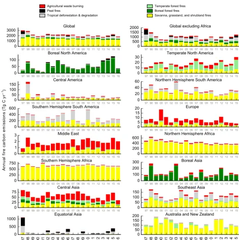
Forest fires are the primary driver of interannual variability in fire emissions (Fig. 9, Table 3). In the tropics, much of this variability is linked with sea surface temperatures, includ-ing large-scale climate modes such as El Niño, which alter fire risk in tropical forests (Chen et al., 2016). El Niño years including 1997–1998, 2002, and 2015 have relatively large contributions from tropical forests. Peat burning in Equato-rial Asia contribute substantially to anomalously high emis-sions 1997 and 2015, in part due to the human-ignited fires that burn in drained peatlands during prolonged drought peri-ods associated with El Niño (Field et al., 2016; van der Werf et al., 2008). Most of the interannual variability in emissions originates from regions outside of Africa, which is shown in the top right panel in Fig. 9.
Tropical deforestation & degradation Savanna, grassland, and shrubland fires Peat fires Boreal forest fires
Agricultural waste burning Temperate forest fires
97 98 99 00 01 02 03 04 05 06 07 08 09 10 11 12 13 14 15 16 0
1000 2000
3000 Global
97 98 99 00 01 02 03 04 05 06 07 08 09 10 11 12 13 14 15 16 0
500 1000 1500
2000 Global excluding Africa
97 98 99 00 01 02 03 04 05 06 07 08 09 10 11 12 13 14 15 16 0
50 100
Boreal North America
97 98 99 00 01 02 03 04 05 06 07 08 09 10 11 12 13 14 15 16 0
10 20
30 Temperate North America
97 98 99 00 01 02 03 04 05 06 07 08 09 10 11 12 13 14 15 16 0
50 100
150 Central America
97 98 99 00 01 02 03 04 05 06 07 08 09 10 11 12 13 14 15 16 0
20 40
60 Northern Hemisphere South America
97 98 99 00 01 02 03 04 05 06 07 08 09 10 11 12 13 14 15 16 0
200 400
600 Southern Hemisphere South America
A
n
n
u
a
l
fi
re
c
a
rb
o
n
e
m
is
si
o
n
s
(T
g
C
y
r
)
–1
97 98 99 00 01 02 03 04 05 06 07 08 09 10 11 12 13 14 15 16 0
5 10 15
20 Europe
97 98 99 00 01 02 03 04 05 06 07 08 09 10 11 12 13 14 15 16 0
1 2
3 Middle East
97 98 99 00 01 02 03 04 05 06 07 08 09 10 11 12 13 14 15 16 0
200 400
600 Northern Hemisphere Africa
97 98 99 00 01 02 03 04 05 06 07 08 09 10 11 12 13 14 15 16 0
250 500
750 Southern Hemisphere Africa
97 98 99 00 01 02 03 04 05 06 07 08 09 10 11 12 13 14 15 16 0
100 200
300 Boreal Asia
97 98 99 00 01 02 03 04 05 06 07 08 09 10 11 12 13 14 15 16 0
25 50
75 Central Asia
97 98 99 00 01 02 03 04 05 06 07 08 09 10 11 12 13 14 15 16 0
50 100
150 Southeast Asia
1997 1998 1999 2000 2001 2002 2003 2004 2005 2006 2007 2008 2009 2010 2011 2012 2013 2014 2015 2016 0
500
1000 Equatorial Asia
1997 1998 1999 2000 2001 2002 2003 2004 2005 2006 2007 2008 2009 2010 2011 2012 2013 2014 2015 2016 0
50 100 150
200 Australia and New Zealand
Figure 9.GFED4s annual fire carbon emissions for various regions and sources.
4.3 Fuel consumption
Modeled and measured (van Leeuwen et al., 2014) fuel con-sumption agree reasonably when aggregated to biome levels (Fig. 12). Fuel consumption in savannas and other regions with herbaceous fuels is lower in GFED4 (both with and without small fires) than in GFED3 because of increases in the turnover rates of herbaceous leaf and surface litter pools. As a consequence, fuel consumption in GFED4 in savannas has decreased 30 % compared to GFED3. Compared with the fuel consumption database from van Leeuwen et al. (2014), GFED4 predicts estimates that are, on average, 14 % higher
than the fuel consumption measured in the collocated grid cells. GFED4 also shows a somewhat lower range than the observations.
1997 2002 2007 2012 2017
0
200
400
600
800
Global
1997 2002 2007 2012 2017
0
200
400
600
800
Emission from GFED4 burned area Emission from GFED4s burned area
Global excluding Africa
1997 2002 2007 2012 2017
0
20
40
60
Boreal North America
1997 2002 2007 2012 2017
0
5
10
15
Temperate North America
1997 2002 2007 2012 2017
0
50
100
Central America
1997 2002 2007 2012 2017
0
10
20
30
Northern Hemisphere South America
1997 2002 2007 2012 2017
0
100
200
300
Mo
nt
hly
fi
re
ca
rb
on
em
iss
ion
s (
Tg
C
m
on
th
−
1
)
Southern Hemisphere South America
1997 2002 2007 2012 2017
0
2
4
6
Europe
1997 2002 2007 2012 2017
0.0
0.5
1.0
Middle East
1997 2002 2007 2012 2017
0
50
100
150
200
Northern Hemisphere Africa
1997 2002 2007 2012 2017
0
100
200
Southern Hemisphere Africa
1997 2002 2007 2012 2017
0
50
100
Boreal Asia
1997 2002 2007 2012 2017
0
10
20
Central Asia
1997 2002 2007 2012 2017
0
50
Southeast Asia
1997
2002
2007
2012
2017
Year
0
200
400
600
Equatorial Asia
1997
2002
2007
2012
2017
Year
0
20
40
60
Australia and New Zealand
Figure 10.Monthly emissions from GFED4 (red) and GFED4s (grey).
back to one very high measurement in Tasmania that is not reproduced in the collocated grid cell in GFED4; the me-dians are in close agreement. Pinpointing the reasons for the disagreement in boreal regions is less straightforward; the range, mean, and medians for the modeled values ex-ceed the measured ones. One potential reason might be re-lated to the relatively large number of experimental burns in the database of van Leeuwen et al. (2014) for this biome, which in general occur under conditions less favorable for large fires to prevent them from growing out of control. For the state of Alaska, GFED4 estimates of fuel consumption are similar to estimates from the Alaska Large Fire Database
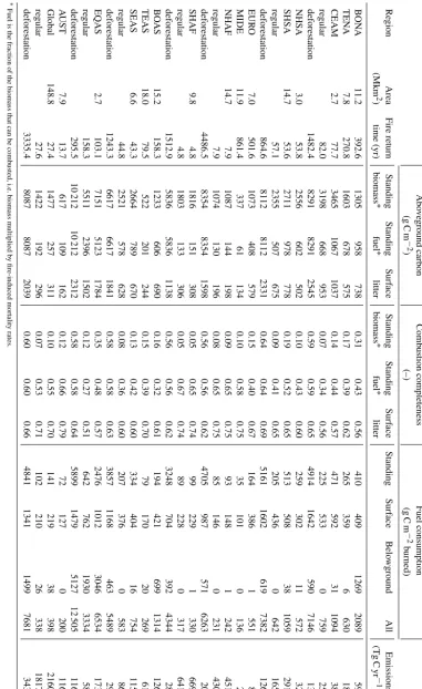
Table 3.Carbon emissions estimates and the contribution of different fire categories over the 1997–2016 study period. Region abbreviations are described in Fig. 3.
Region Carbon emissions (Tg C yr−1) CV (%) Contribution of different fire categories to total carbon emissions (%)
Mean Minimum Maximum Savanna Boreal Temperate Tropical Peat Agriculture
forest forest forest
BONA 59 12 128 53 0.3 86.5 4.2 0.0 7.3 1.7
TENA 18 11 31 28 33.2 0.0 46.4 0.0 0.0 20.3
CEAM 38 15 177 92 45.5 0.0 1.9 36.7 0.0 15.9
NHSA 32 13 60 36 71.1 0.0 0.0 23.0 0.0 5.9
SHSA 291 104 561 44 49.3 0.0 1.8 45.7 0.0 3.2
EURO 8 4 19 43 29.0 0.2 12.2 0.0 0.0 58.6
MIDE 2 1 3 24 35.8 0.0 3.4 0.0 0.0 60.8
NHAF 451 359 645 16 88.3 0.0 0.0 5.2 0.0 6.5
SHAF 669 583 774 7 92.4 0.0 0.1 4.8 0.0 2.7
BOAS 126 45 280 51 2.0 79.5 2.5 0.0 1.7 14.3
TEAS 61 36 85 23 29.8 11.4 12.7 2.4 0.0 43.6
SEAS 115 66 177 28 53.4 0.0 7.1 31.3 0.0 8.3
EQAS 173 18 1110 139 11.2 0.0 0.0 43.7 42.8 2.2
AUST 116 42 190 35 86.3 0.0 9.9 2.3 0.0 1.5
Global 2160 1773 3032 15 65.3 7.4 2.3 15.1 3.7 6.3
4.4 Greenhouse gas forcing of fires and potential for mitigation
Fires emit the greenhouse gases CO2, CH4, and N2O and
also modify the climate by emitting precursors of aerosols and ozone, aerosols, and changing surface properties such as albedo in often complex ways (Randerson et al., 2006; Ward et al., 2012). Average total annual greenhouse gas emis-sions according to GFED4s were 7.3 Pg CO2, 16 Tg CH4,
and 0.9 Tg N2O. Note that in this section we refer to C
emis-sions in CO2 mass units rather than the C mass units used
in the rest of the paper. Using a 100-year time horizon and based on global warming potentials of 34 for CH4and 298
for N2O (Myhre et al., 2013), this translates to 8.1 Pg CO2
equivalent annually, or 23 % of global fossil fuel CO2
emis-sions in 2014 (Boden et al., 2017; Le Queré et al., 2015). However, fire emissions are not generally a net CO2source
to the atmosphere, and may be better viewed as “fast respi-ration”, because regrowing vegetation in many burned areas will sequester a roughly equivalent amount of atmospheric CO2during post-fire stages of ecosystem recovery over a
pe-riod of years to decades (Landry and Matthews, 2016). In general, only fires that are not balanced by regrowth are a net CO2source. The most obvious fire types in this category
are fires used in the deforestation process or those that burn drained peatlands. CO2emissions from these two fire types
are estimated here to be 0.4 Pg C or 1.3 Pg CO2per year.
In-cluding CH4 and N2O of all fire types, the contribution of
fires to the greenhouse gas budget is 2.1 Pg CO2equivalent
annually or 6 % of global fossil fuel CO2emissions in 2014
(Boden et al., 2017). Another category of fire emissions that may add to the build-up of atmospheric CO2are those that
O N D J F M A
Month
0
20
40
60
80
100
120
140
160
180
Em
iss
ion
s (
Tg
C
m
on
th
−
1
)
(a) NHAF
Previous
Modified
M J J A S O N
Month
0
20
40
60
80
100
120
140
160
180
(b) SHAF
Figure 11.Monthly GFED4s fire carbon emissions for Northern Hemisphere Africa(a)and Southern Hemisphere Africa(b)based on straight conversion of burned area to burned fraction (“pre-vious”) and with the new parameterization according to Eq. (3) (“modified”).
increase over time, for example increasing burned area or combustion completeness in boreal regions related to climate change. Our time series is too short and our modeling frame-work is too incomplete to capture the exact magnitude of emissions from a changing boreal fire regime.
Savanna fire season management has been proposed as a climate mitigation instrument (Russell-Smith et al., 2013). By burning early in the season instead of late, fires are in gen-eral more patchy, release fewer emissions, and prevent large late-season fires. According to GFED4s, total annual trop-ical savanna fire emissions averaged 4.9 Pg CO2, 6 Tg CH4,
and 0.6 Tg N2O. In this case, only CH4and N2O emissions
50 100 200 500 1000 2000 5000 10 000 20 000
18 1.45
27 0.67
16 1.39
4 1.11
3 0.32
1 0.79
1 0.92 n: 105
Ratio of means: 1.14
Savanna Tropical forestTemperate forestBoreal forestAgriculture Tropical peatBoreal peatTundra
Measurements:
GFED4:
F
ue
l c
on
su
m
pt
io
n
(g
C
m
–
2 bu
rn
ed
)
Figure 12. Measured and modeled fuel consumption for various biomes showing the range (whiskers), mean (colored dots and di-amonds), median (open dots and didi-amonds), and 25th and 75th percentiles (boxes) for those biomes with more than 10 measure-ments. Comparison is based on the meta-analysis of van Leeuwen et al. (2014) and collocated 0.25◦ grid cells. The time periods of measurement and model do not necessarily overlap. “n” indicates the number of measurements for each biome. Note the logarithmic scale.
of annual emissions. Experiments with early burning in Aus-tralia have shown a potential reduction of up to 50 % (Walsh et al., 2014), but it is not known to what extent it is possible to use this approach in other regions, what the side effects will be, and whether some of the mitigation will be offset by higher CH4 emission factors because early season fires
may occur when fuels have had less time to cure. In Aus-tralia the latter is probably not the case (Meyer et al., 2012), but whether this is found in other regions remains to be in-vestigated.
4.5 Differences between GFED4s, GFED4, and GFED3
In general, small fire burned area (GFED4s) and the modi-fied burned-area-to-burned-fraction conversion (GFED4 and GFED4s) cause emissions to increase, while the optimization of fuel consumption causes emissions to decrease as com-pared with earlier versions of GFED. On a global scale, these modifications yield a modest net increase in fire carbon emis-sions in GFED4s as compared with GFED3 (11 % for the overlapping 1997–2011 time period). However, the effects of the three main adjustments vary spatially; on a regional scale the differences are larger (Fig. 13). The relative effect of the small fire burned area is largest in temperate and sub-tropical regions where agricultural waste burning and shift-ing cultivation are important drivers of fire activity. The more than doubling of burned area in Central America and
North-ern Hemisphere South America compared to GFED3 reflects differences in both GFED4 burned area and the inclusion of small fires (Fig. 13). Burned area in Temperate North Amer-ica and Europe also increases by about a factor of 2, and most of this difference is due to small fire burned area.
Our modifications to herbaceous fuel turnover rates cause fuel consumption per unit area (per m2 of burned area) to decrease, whether or not small fire burned area is included, in all regions except Central Asia, where consumption in-creased by approximately 20 to 30 % (Fig. 13). Estimates of fuel consumption per unit area are similar in GFED4 and GFED4s, indicating that fuel loads in areas burned by small fires are not substantially different from those in nearby mapped burned areas (or that our relatively coarse model-ing setup cannot resolve finer-scale landscape differences). The exception is Central Asia, where small fire burned area causes a relative increase in burned area in forested regions. In Central America and Equatorial Asia, in contrast, small fire burned area occurs predominantly in areas with relatively low fuel loads.
The modified burned-area-to-burned-fraction parameteri-zation causes an increase of 5 % in carbon emissions (not shown). The new parameterization only influences grid cells that burn for more than 1 month in a season, and has a larger effect in grid cells that have a high burn fraction. Regions with frequent savanna fires therefore have the highest sensi-tivity, with emissions in Northern Hemisphere Africa, South-ern Hemisphere Africa, and Australia increasing by 9, 8, and 6 %, respectively. In other regions, the differences are smaller than 2 %. In addition to the increase in emissions in frequently burning savannas, the new parameterization also changes the temporal dynamics (Fig. 11); early season emis-sions are lower because less fuel remains from the previous growing season, and late-season emissions are higher be-cause the parameterization has the effect of increasing grid-cell level fuel consumption later in the fire season.
Without small fire burned area, the impact of decreas-ing fuel consumption and a minor reduction in burned area (2 % globally) yields a total carbon emissions estimate of 1.5 Pg C yr−1 in GFED4, a 23 % reduction compared to GFED3 during 1997–2011. Although globally GFED4 emis-sions are lower than GFED3, in some regions both burned area and emissions increase, mostly in temperate regions (Fig. 13). Using the new set of emission factors that sepa-rate extratropical forests into boreal forest and tempesepa-rate for-est components generates a larger increase in CO emissions in boreal regions than expected from the change in carbon emissions alone (Fig. 14).
5 Discussion
50 0 50 100 150 200
BONA TENA CEAM NHSA SHSA EURO MIDE NHAF SHAF BOAS CEAS SEAS EQAS AUST Global
GFED4
GFED4s
Burned area
40 20 0 20
BONA TENA CEAM NHSA SHSA EURO MIDE NHAF SHAF BOAS CEAS SEAS EQAS AUST Global
Difference between GFED4 (grey) or GFED4s (black) and GFED3 (%), averaged over the 1997–2011 period Fuel consumption
60 30 0 30 60 90 120
BONA TENA CEAM NHSA SHSA EURO MIDE NHAF SHAF BOAS CEAS SEAS EQAS AUST Global
Carbon emissions
60 30 0 30 60 90 120
CO emissions
Figure 13. Relative differences in burned area, fuel consumption per unit burned area, carbon emissions, and carbon monoxide (CO) emissions between GFED4 (black) and GFED4s (grey) compared to GFED3 for 14 basis regions explained in Fig. 3 and the globe averaged over 1997 to 2011.
70◦N 50◦N 30◦N 10◦N 10◦S 30◦S 50◦S
Latitude 0
1 2 3 4 5
C
O
e
m
is
si
o
n
s
(g
C
O
m
–2
y
r
)
–1
GFED3 GFED4 GFED4s
Figure 14.Latitudinal distribution of carbon monoxide (CO) emis-sions for GFED3, GFED4, and GFED4s.
variations in environmental conditions. In a subsequent step, we have used a higher-resolution set of emission factors to convert carbon emissions into emissions of trace gases and aerosols. Since the publication of GFED3 in 2010, burned area algorithms have been improved considerably (Giglio et al., 2013), and now include a preliminary estimate of the impact of small fires (Randerson et al., 2012). In parallel, the fuel consumption database created by van Leeuwen et al. (2014) has enabled the development of an improved pa-rameterization of herbaceous vegetation turnover in
grass-land and savanna ecosystems, and validation of our modeled values in several other biomes. New emission factor mea-surements and a more systematic assessment of the available data has led to a more consistent set of emission that bet-ter resolve extratropical forest biomes (Akagi et al., 2011). Together, all of the elements required to calculate emissions following the Seiler and Crutzen (1980) paradigm have seen substantial improvements. Our new emission estimates are therefore more reliable than previous estimates because they account for updated information on key components of the fire emissions equation, but uncertainties remain substantial and are difficult to quantify.
The addition of small fire burned area is a key improve-ment in GFED4s compared to earlier versions, for example, and the modifications we describe in this paper have im-proved our estimates compared to Randerson et al. (2012). However, the actual magnitude of small fire burned area is difficult to quantify on global scales because it requires a large sample of burned area measurements from sensors with a higher spatial resolution than MODIS. To date, Landsat es-timates of burned area have been produced for various re-gions and purposes including the validation of coarser res-olution data (Padilla et al., 2014, 2015; Roy and Boschetti, 2009; Silva et al., 2005) but a publicly available and global-scale database of Landsat burned area is needed to better validate ongoing efforts to produce reliable burned area esti-mates from coarser resolution satellite imagery. In addition, new missions such as the Visible Infrared Imager Radiome-ter Suite (VIIRS) and Landsat-8 also increase the number of active fires detected compared to MODIS (Schroeder et al., 2014b).
Leeuwen et al. (2014) has enabled a more systematic valida-tion but the number of studies is limited, relatively few mea-surements were made during our study period, and it is ques-tionable to what degree the local measurements are represen-tative for the 0.25◦ grid cell averages reported here. Thus, our estimates are likely to remain most useful for large-scale studies. Although recent regional studies have shown that our global modeling framework is indeed capable of generating reliable large-scale emissions in Alaska and the tropics, these studies also show that GFED may have problems capturing finer-scale dynamics (Andela et al., 2016; Veraverbeke et al., 2015). While improved satellite missions and combining var-ious data streams may help in improving the fuel consump-tion parameterizaconsump-tion in models, systematic field-based as-sessments of fuel consumption along gradients of productiv-ity and other factors influencing variabilproductiv-ity in fuel consump-tion within biomes are a necessary step in further improving bottom-up fire emission estimates. New satellite estimates of biomass may be helpful in this regard (for example the Global Ecosystem Dynamics Investigation (GEDI) mission), particularly in deforestation and temperate forest and shrub-land regions, where aboveground living biomass comprises a large component of fuel consumption.
Given the large uncertainties in bottom-up emission esti-mates in the past, top-down constraints have often been used to pinpoint discrepancies between modeled and measured atmospheric abundances of trace gases or aerosols. Carbon monoxide (CO) was most often used (Arellano et al., 2004; Hooghiemstra et al., 2011; Huijnen et al., 2016) because fires are a major source of CO, its lifetime is relatively long, and column CO is measured from several satellite sensors. More recent work also includes other species such as formalde-hyde, NO2, and aerosol optical depth (Bauwens et al., 2016;
Mebust et al., 2011; Petrenko et al., 2012). While provid-ing additional information on strengths and weaknesses of inventories such as GFED, for example potentially missing late-season fires (Castellanos et al., 2014), the results of these studies are often contradicting (van Leeuwen et al., 2013), potentially due to the use of different atmospheric models and sources of observations. We would therefore respect-fully argue that uncertainties in bottom-up and top-down ap-proaches are overlapping. For example, carbon emissions from Indonesia during the 2015 high fire year according to GFED4s were almost 400 TgC (Fig. 9, http://www.geo.vu.nl/ ~gwerf/GFED/GFED4/tables/GFED4.1s_C.txt). Two inver-sion studies using Measurement of Pollution in the Tropo-sphere (MOPITT) CO measurements derived either 100 Tg higher (Yin et al., 2016) or 100 Tg lower (Huijnen et al., 2016). Part of the difference can be attributed to the use of higher CO emission factors in the latter study, which thus re-quires less carbon burned to match atmospheric observations, but part is also due to differences in model setup and analy-sis design. The use of different top-down constraints (e.g. In-frared Atmospheric Sounding Interferometer (IASI) versus MOPITT) could lead to additional discrepancies, although
studies employing column CO2 from the Orbiting Carbon
Observatory-2 (OCO-2) may omit some of the issues related to uncertainty in emission factors. Heymann et al. (2017) pro-vided evidence for lower estimates than found in GFED4s in Indonesia for 2015 based on OCO-2 data.
Studies focusing on aerosol optical depth (AOD) do not give conflicting results but indicate that bottom-up estimates are roughly a factor 3 too low (Johnston et al., 2012; Kaiser et al., 2012; Petrenko et al., 2012; Tosca et al., 2013). While some studies have therefore boosted bottom-up emissions or created new inventories with much higher emissions to get AOD values more in line with observations (Liousse et al., 2010), this may jeopardize the reasonable agreement between bottom-up and top-down estimates found for most trace gases. To date, the disagreement between measured and modeled AOD has most often been linked to bottom-up emis-sions, but AOD calculation in models are uncertain as well. For example, increasing the hygroscopicity reduced the off-set in tropical regions (Reddington et al., 2016). Besides ex-ploring the factors that are used to estimate AOD in models such as the hygroscopicity, combining multiple species in in-version studies and better emission factors are needed to re-solve one of the most important questions in biomass burning emissions research.
Most of the emission factors (EFs) used in these top-down approaches are based on midday sampling during peak fire emission rates. The EFs measured under these somewhat re-stricted circumstances are still highly variable with a coef-ficient of variation about the mean of about 40 % on aver-age (Akagi et al., 2011). The diurnal or longer-term varia-tion in EFs should be larger but has not been explicitly well-measured yet (Saide et al., 2015). The EFs of many species have rarely been measured in the field for important fire types such as wildfires (Akagi et al., 2011) and for some compound classes with perhaps the most important missing species be-ing the semi-volatile precursors to organic aerosol, which are difficult to measure even in lab experiments (Gilman et al., 2015). A related area of uncertainty is the temporal evolution of emissions within the fire plume. Only a few field studies have measured how organic aerosol (OA) levels change with time. In one an increase in OA by a factor of about 2.5 was observed (Yokelson et al., 2009), while in another study OA decreased by about 20 % (Akagi et al., 2012). Understand-ing what controls secondary OA levels is critical to guide the proper use of AOD in inversions and to understand health and climate impacts.
burn preferentially leading to underestimated EFs if based on average fuel C content (Santin et al., 2015). In general these small uncertainties may tend to cancel out. EFs may also be systematically overestimated by 1–3 % because many carbon-containing species cannot yet be measured (Akagi et al., 2011).
For GFED3, we performed a Monte Carlo simulation to estimate carbon emissions uncertainties based on assumed uncertainties of key input data including burned area and best-guess estimates of various model parameters. We now refrain from estimating formal uncertainties because of dif-ficulties in assessing the uncertainties in the various layers. For example, the burned area in many regions where small fires seem to be important now by far exceeds the range of uncertainty reported for GFED3 burned area. Given the level of agreement between our burned area estimates and more refined regional estimates (Randerson et al., 2012), and between our modeled biome-average fuel consumption esti-mates and those measured in the field, a best-guess uncer-tainty assessment at regional scales could be a 1σ of about 50 % in general but higher in areas where small fire burned area is important or where there is significant fuel consump-tion in organic soils.
Lowering and/or better quantifying this uncertainty in-volves a thorough assessment of the burned area estimates and especially those from small fires, using more direct satel-lite observations of fire severity and fuel consumption based on FRP data, and new field data on fuel consumption and emission factors along critical gradients such as productiv-ity and grazing intensproductiv-ity. Increasing the spatial resolution of our modeling framework could lower the impact of spatial heterogeneity in fire parameters and make for easier com-parisons with or validation using ground-based data. Better understanding and modeling diurnal cycles may be equally important in addressing how variable, for example, the rela-tive importance of flaming and smoldering combustion is. Fi-nally, with new missions such as Suomi-NPP and the various Sentinel satellites now collecting data, an emphasis on merg-ing various time series would help in lengthenmerg-ing the time series over which we have consistent data to over 20 years.
6 Data availability
GFED data are freely available at http://www.globalfiredata. org. The site provides documentation, related publications, updates, and online analysis tools to compute emissions for custom regions and countries.
7 Conclusions
We have revised the Global Fire Emissions Database us-ing new observations of burned area includus-ing those from smaller fires as well as several other new data streams. In ad-dition we have modified the fuel consumption
parameteriza-tion in our model to better match observaparameteriza-tions. Global aver-age fire emissions were estimated to be 2.2 Pg C yr−1 over
1997–2016 with substantial interannual variability. This is an 11 % increase compared to our previous work (GFED3), and in regions where small fires are relatively important such as temperate cropland regions the increase could be as large as 100 %. Net greenhouse gas emissions from all fires were on average 6 % of global 2014 fossil fuel CO2 emissions,
consisting of 0.4 Pg C yr−1emissions from deforestation and tropical peat fires, which are a net CO2 source to the
at-mosphere just like fossil fuel emissions, and 16 Tg CH4and
0.9 Tg N2O yr−1from all fire types using a 100-year horizon
to convert the warming potential of these greenhouse gases to CO2equivalents.
Over the past several years, uncertainties in all of the data layers used to calculate emissions (burned area, fuel con-sumption, and emission factors) have been reduced from new algorithms and data availability. While biome-level fuel con-sumption rates are now more in line with observations than in our previous work, uncertainties are still substantial at higher resolutions as indicated by regional studies. In ad-dition, the small fire burned area approach carries substan-tial uncertainties and is known to be impacted by resam-pling error. Merging information from the long-term MODIS era with newer instruments could reduce some of these un-certainties, but carefully designed and interdisciplinary field campaigns measuring fuel consumption, fire dynamics, and emission factors along gradients and throughout fire seasons are equally necessary to further improve biomass burning es-timates.
Competing interests. The authors declare that they have no con-flict of interest.
Acknowledgements. This research was supported by the European Research Council (ERC) grant number 280061, the Gordon and Betty Moore Foundation (GBMF3269), NASA (NNX14AP45G), the U.S. National Science Foundation, and the EU H2020 Monitoring Atmospheric Chemistry and Climate (MACC-III) project.
Edited by: Vinayak Sinha
Reviewed by: two anonymous referees
References
Akagi, S. K., Yokelson, R. J., Wiedinmyer, C., Alvarado, M. J., Reid, J. S., Karl, T., Crounse, J. D., and Wennberg, P. O.: Emis-sion factors for open and domestic biomass burning for use in atmospheric models, Atmos. Chem. Phys., 11, 4039–4072, https://doi.org/10.5194/acp-11-4039-2011, 2011.