www.geosci-model-dev.net/6/1641/2013/ doi:10.5194/gmd-6-1641-2013
© Author(s) 2013. CC Attribution 3.0 License.
Geoscientific
Model Development
A refined statistical cloud closure using double-Gaussian probability
density functions
A. K. Naumann1,2, A. Seifert3, and J. P. Mellado1
1Max Planck Institute for Meteorology, 20146 Hamburg, Germany
2International Max Planck Research School on Earth System Modelling (IMPRS-ESM), Max Planck Institute for Meteorology, 20146 Hamburg, Germany
3Hans-Ertel Centre for Weather Research, Deutscher Wetterdienst, 20146 Hamburg, Germany Correspondence to: A. K. Naumann ([email protected])
Received: 18 January 2013 – Published in Geosci. Model Dev. Discuss.: 18 February 2013 Revised: 12 August 2013 – Accepted: 2 September 2013 – Published: 8 October 2013
Abstract. We introduce a probability density function (PDF)-based scheme to parameterize cloud fraction, average liquid water and liquid water flux in large-scale models, that is developed from and tested against large-eddy simulations and observational data. Because the tails of the PDFs are cru-cial for an appropriate parameterization of cloud properties, we use a double-Gaussian distribution that is able to repre-sent the observed, skewed PDFs properly. Introducing two closure equations, the resulting parameterization relies on the first three moments of the subgrid variability of temperature and moisture as input parameters. The parameterization is found to be superior to a single-Gaussian approach in diag-nosing the cloud fraction and average liquid water profiles. A priori testing also suggests improved accuracy compared to existing double-Gaussian closures. Furthermore, we find that the error of the new parameterization is smallest for a hori-zontal resolution of about 5–20 km and also depends on the appearance of mesoscale structures that are accompanied by higher rain rates. In combination with simple autoconversion schemes that only depend on the liquid water, the error in-troduced by the new parameterization is orders of magnitude smaller than the difference between various autoconversion schemes. For the liquid water flux, we introduce a parame-terization that is depending on the skewness of the subgrid variability of temperature and moisture and that reproduces the profiles of the liquid water flux well.
1 Introduction
The cloud fraction and the average liquid water in a given volume depend on the variability of temperature and mois-ture within that volume. If subgrid variability is not taken into account at all, the grid volume is either entirely subsat-urated or entirely satsubsat-urated. To overcome this problem, di-agnostic relative humidity schemes have been developed, for example by Smagorinsky (1960) and Sundqvist et al. (1989) who parameterized partial cloud fraction as a function of relative humidity with a certain critical relative humidity at which a partial cloud cover first appears. This kind of pa-rameterization has been developed further by implementing secondary predictors like condensate content (e.g., Xu and Randall, 1996) or vertical velocity (e.g., Slingo, 1987).
Another approach in diagnosing cloud fraction is based on one-dimensional probability density functions (PDFs) of the subgrid variability in temperature and moisture1. Assuming a single-Gaussian PDF, these schemes go back to Somme-ria and Deardorff (1977) and Mellor (1977) and need not only the grid-box mean temperature and moisture but also the standard deviations as input parameters. Because the success of such schemes crucially depends on the ability to quan-tify the tails of the distribution (Bougeault, 1982a), further studies additionally took into account the skewness of the 1Assuming a uniform PDF of the total water subgrid-scale
vari-ability and the variance as a constant fraction of the saturation value, it has been shown (e.g., by Quaas, 2012), that the Sundqvist et al. (1989) relative humidity scheme is a special case of PDF-based schemes.
1642 A. K. Naumann et al.: A refined statistical cloud closure
distribution which lead to the use of, for example, double-Gaussian (Lewellen and Yoh, 1993; Larson et al., 2001a), Gamma (Bougeault, 1982b) or Beta (Tompkins, 2002) distri-butions. Perraud et al. (2011) tested several of this distribu-tions against model data and found that the double-Gaussian distribution gives best results.
Compared to relative humidity schemes, PDF-based schemes typically need more and higher moments as in-put parameters. While the first two moments are commonly available in numerical weather prediction (NWP) models and general circulation models (GCMs), there are ongoing ef-forts to develop higher-order closure boundary layer models which include an estimate of the third moment, that is, the skewness (Gryanik and Hartmann, 2002; Gryanik et al., 2005; Mironov, 2009; Machulskaya and Mironov, 2013). Apart from this disadvantage, PDF schemes have several ad-vantages over relative humidity schemes. In PDF schemes, the shape of the PDF is parameterized but the variables aimed for, such as cloud fraction and average liquid water, are derived directly from this PDF. Therefore, the variables are calculated consistently from the assumed PDF. Also, nu-merical models that ignore subgrid variability are known to encounter systematic errors in cloud and radiative proper-ties (Pincus and Klein, 2000; Rotstayn, 2000; Larson et al., 2001b). To tackle this issue, the knowledge of the subgrid PDF is essential. Furthermore, PDF schemes can potentially be used in a wide range of cloud regimes. Other than for rel-ative humidity schemes, no trigger functions to switch from one regime (and its according parameterization) to another regime are needed and artificial distinctions can be avoided.
As a further development from one-dimensional PDFs, joint PDFs have been introduced recently (e.g., by Larson et al., 2002). In joint-PDF schemes the variability of tem-perature and moisture are usually not summarized in one variable and the distribution of the vertical velocity can be added as further input. Because the vertical velocity is taken into account, the liquid water flux can be derived consis-tently from the joint PDF. This advantage has to be paid for by the prediction or diagnosis of several more moments and correlations among temperature, humidity and vertical velocity (e.g., Larson et al., 2002, used 19 parameters in-stead of 5 for a double-Gaussian distribution). Hence joint-PDF schemes are much more computational expensive than one-dimensional PDF schemes and their usage in operational NWP models or GCMs is challenging with todays computa-tional power.
We therefore step back to one-dimensional PDF schemes and focus on improving the double-Gaussian PDF scheme to diagnose subgrid cloud fraction and average liquid water. The formulation follows Larson et al. (2001a) and is devel-oped from and tested against large-eddy simulations (LES) as well as aircraft measurements. In Sect. 2, the LES model, the case studies the model is applied to and the observa-tional data set are described. The use and construction of a double-Gaussian PDF, the refined closure equations and the
parameterization of the liquid water flux are introduced in Sect. 3. Next, in Sect. 4, we perform a priori testing of the new cloud closure with LES data as input to examine the pa-rameterization’s behaviour under idealized conditions, that is, excluding the interplay with other model components as would be done with a posteriori testing in an NWP model or a GCM. In the following Sects. 5 and 6, the error depen-dence of the parameterization on domain size and the role of mesoscale structures are discussed and the introduced cloud closure is extended to the diagnosis of the autoconversion rate. Finally, in Sect. 7, we give some concluding remarks.
2 Model and data
2.1 Large-eddy simulations
The LES model used in this study is the University of California, Los Angeles LES (UCLA-LES; Stevens et al., 2005; Stevens, 2007) with one major difference to previous work, that is, the time stepping is done with a third-order Runge–Kutta scheme instead of the former leapfrog scheme. Prognostic equations for each of the following variables are solved: the three components of the velocity, the total wa-ter mixing ratio, the liquid wawa-ter potential temperature, the mass mixing ratio of rain water and the mass specific number of rain-water drops. Considering only warm clouds, we use the double-moment bulk microphysical scheme from Seifert and Beheng (2001). Subgrid fluxes are modelled with the Smagorinsky–Lilly model.
For our study, we adapt the UCLA-LES to four differ-ent case studies which span over a range of differdiffer-ent cloud regimes. Shallow cumulus over ocean (RICO2; see Rauber et al., 2007) and over land (ARM3; see Brown et al., 2002) are considered as well as stratocumulus (DYCOMS4; see Stevens et al., 2003) and the transition from stratocumulus to cumulus (ASTEX5; see Albrecht et al., 1995). Domain sizes and resolutions of the different LES cases are given in Ta-ble 1.
2.1.1 ARM
The LES setup of the ARM case follows that of the sixth in-tercomparison project, performed as part of the GCSS6 pro-gram and described by Brown et al. (2002).
2.1.2 ASTEX
The setup of the LES study for the ASTEX case is similar to that proposed by the Euclipse ASTEX Lagrangian model
2Rain in cumulus over the ocean 3Atmospheric radiation measurement
4Dynamics and chemistry of marine stratocumulus 5Atlantic stratocumulus transition experiment
6GEWEX (Global Energy and Water Experiment) Cloud system
Table 1. Overview of the different LES cases used in this study. The four cases on the left hand side are used to develop (DYCOMS and
RICO) and test (ARM and ASTEX) the parameterizations introduced in this study. The three cases on the right hand side are solely used in the Sect. 5.
ARM ASTEX DYCOMS RICO RICO
standard standard moist moist
nx 256 256 512 512 1024 1024 2048
L 12.8 km 10.2 km 10.2 km 20.5 km 25.6 km 25.6 km 51.2 km
H 5.1 km 3.2 km 1.4 km 4.0 km 4.0 km 4.0 km 4.0 km
1x 50 m 40 m 20 m 40 m 25 m 25 m 25 m
1z 40 m 20 m 5–52 m 20 m 25 m 25 m 25 m
t 15 h 42 h 5 h 36 h 30 h 30 h 30 h
nx: number of grid points in each horizontal direction,L: horizontal domain size,H: vertical domain size,1x: horizontal resolution,1z: vertical resolution,t: length of simulation.
intercomparison case (van der Dussen et al., 2013). The ini-tial profiles are identical to the first GCSS ASTEX “A209” modelling intercomparison case and the model is forced by time-varying sea surface temperature and divergence taken from Bretherton et al. (1999).
2.1.3 DYCOMS
For the LES setup of DYCOMS, we follow the DYCOMS-II RF01 setup of the eighth case study conducted under the auspices of the GCSS boundary layer cloud working group and described by Stevens et al. (2005).
2.1.4 RICO
The initial data and the large-scale forcing for the standard RICO simulations are based on the precipitating shallow cu-mulus case that was constructed by the GCSS boundary layer working group and described by van Zanten et al. (2011). A modified moister version, which differs from the stan-dard setup only by a moister initial profile, was first used by Stevens and Seifert (2008), to which we refer for a de-tailed setup of the case. The moister initial condition leads to higher rain rates compared to the standard case and sub-sequently to mesoscale organization of the cloud field due to the formation of cold pools mainly caused by evaporation of rain in the sub-cloud layer (Seifert and Heus, 2013).
Unless stated otherwise, we refer to our standard RICO setup with nx=512 when analysing LES data from the RICO case. The three RICO cases on the right hand side in Table 1 are equal to the LES runs R01, M01 and M01bigof Seifert and Heus (2013). For this study they are solely used in Sect. 5 when discussing the error dependence on domain size and the role of mesoscale structures.
2.2 Observational data
To be able to test our parameterization against observa-tional data, we used RICO field campaign data (Rauber et al., 2007). This data set includes airborne measurements
obtained from the NSF/NCAR Research Aviation Facility C-130Q Hercules aircraft (Tail Number N130AR) at 25 Hz. Besides the static pressure and the ambient temperature, the water vapor mixing ratio measured with a Lyman-alpha hy-grometer as well as the liquid water content measured with a Gerber PV-100 probe were used in this study. Because the temperature sensor is susceptible to wetting during cloud penetrations, periods of cloud presence were defined by a threshold value of 10 cloud droplets (3 to 45 µm diameters) per cm3and in-cloud temperature was measured by a radio-metric temperature sensor that is not sensitive to wetting. In 17 research flights (RF01 to RF13 and RF16 to RF19) all available five-minutes intervals at moderate height (pressure >600 hPa) and with relatively constant pressure (standard deviation <1 hPa) were selected and analysed. (Note that, unfortunately, during research flight 14 and 15 the Lyman-alpha hygrometer was out of service, so no analysis of these flights is possible.)
3 Introducing a refined cloud closure
3.1 Data analysis: the double-Gaussian PDF
For diagnosing the cloud fraction and the average liquid wa-ter, Perraud et al. (2011) show that the temperature variability should not be neglected relative to the humidity variability. We therefore follow Sommeria and Deardorff (1977), Mellor (1977) and Lewellen and Yoh (1993) and define the extended liquid water mixing ratio,s(qt, Tl), by
s= qt−qs(Tl)
1+L
cp
∂q
s
∂T
T=Tl
, (1)
whereqt is the total water mixing ratio,qs(Tl)is the satu-ration mixing ratio at a given value of the liquid water tem-peratureTl=θlT /θand(∂qs/∂T )T=Tl =Lqs(Tl)/(RvT
2 l )is the slope of the saturation mixing ratio at T =Tl.T is the temperature,θthe potential temperature,θlthe liquid water
1644 A. K. Naumann et al.: A refined statistical cloud closure
potential temperature,Lthe latent heat of vaporization,cp
the specific heat at constant pressure and Rv the gas con-stant for water vapor. The extended liquid water mixing ratio takes into account the temperature variability as well as the humidity variability and is a measure of subsaturation ifs is negative. Fors >0,sis approximately equal to the liquid water mixing ratio,ql. Note that the ratio of the mean ofs, s, to the standard deviation ofs,σ, can be approximated by the normalized saturation deficit,Q1, which is defined as the bulk value ofs,sbu=s(qt,Tl), divided byσ (Lewellen and Yoh, 1993,ζ therein).
If the PDF of s is known for each grid box in an NWP model or a GCM, the cloud fraction and the average liquid water can be calculated by integration over the PDF ofs(see Eqs. 8 and 9 for the formulation of the integral). As this is not the case, and only the first moments of the PDF ofs can usually be predicted in large-scale models, we are using high-resolution LES and observational data to investigate the behaviour of the distribution ofson the subgrid scale of an NWP model or a GCM.
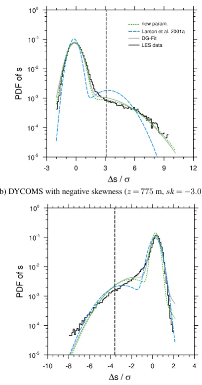
Considering the distribution ofsfrom each model level in the LES data over the whole domain, we find that the PDF of scan be highly skewed in the cloud layer with positive skew-ness for shallow cumulus and negative skewskew-ness for stra-tocumulus (Fig. 1). For shallow cumulus, cloud formation is driven by surface heat fluxes that initiate few but strong updrafts in a slowly descending environment. Therefore the PDF ofsis positively skewed with the moist tail representing the (cloudy) updrafts. In contrast, stratocumulus is driven by radiative and evaporative cooling at cloud top. Hence non-cloudy downdrafts emerge in a dry tail of the PDF ofs and the PDF tends to be skewed negatively (Helfand and Kalnay, 1983; Moeng and Rotunno, 1990). Consequently for both the shallow cumulus regime and the stratocumulus regime, the success of a scheme diagnosing the cloud fraction and the average liquid water depends crucially on its ability to quan-tify the tail of the distribution.
Following Larson et al. (2001a), we choose to represent the PDF ofs by a double-Gaussian distribution which can represent skewed distributions and is able to reproduce the tail. The double-Gaussian distribution is quite popular (Lar-son et al., 2001a; Perraud et al., 2011) because the two single-Gaussian distributions that the double-single-Gaussian distribution is composed of can be interpreted physically as the updrafts and their slowly descending environment in case of a cumu-lus regime (Neggers et al., 2009) or as the downdrafts and their well-mixed environment in the case of a stratocumulus regime. In both regimes the dominant mode of the PDF ofsis associated with the well-mixed environment and assumed to be Gaussian distributed. The tail of the PDF is represented in a secondary mode and is associated with the thermal updrafts in shallow cumulus and the negatively buoyant downdrafts in stratocumulus (Fig. 1). This secondary mode is also assumed to be Gaussian distributed.
a) RICO with positive skewness (z= 1170m,sk= 3.4)
b) DYCOMS with negative skewness (z= 775m,sk=−3.0)
Fig. 1.PDF ofsfor a specific height in the cloud layer. Furthermore, the corresponding best skewness-retaining double-Gaussian fit (DG-Fit) and the resulting PDF when using the closure equations from Larson et al. (2001a)
(Eq. 3) and the introduced closure equations (Eq. 4) are shown. It is∆s=s−s. The black, dashed line indicates
the saturation value (s=0).
25
Fig. 1. PDF ofsfor a specific height in the cloud layer. Further-more, the corresponding best skewness-retaining double-Gaussian fit (DG-Fit) and the resulting PDF when using the closure equations from Larson et al. (2001a) (Eq. 3) and the introduced closure equa-tions (Eq. 4) are shown. It is1s=s−s. The black, dashed line indicates the saturation value (s=0).
Fig. 2.PDF ofsfrom LES data of DYCOMS and from a DNS study. Both PDFs are calculated at a height level
close to the cloud top where the variance of horizontal winds are at their respective maximum. The DNS data
corresponds to a local study of turbulent mixing at cloud top, due solely to evaporative cooling (Mellado et al.,
2010).
a) LES data forσ1 b) LES data forσ2 c) observational data forσ1
Fig. 3. LES data of ARM, ASTEX, RICO and DYCOMS and observational data from the RICO campaign
along with the closure equations from Larson et al. (2001a) (dashed line) and the new closure equations (solid
line). Note that the new closure equations are fitted to the LES data of RICO and DYCOMS rather than to all
available case studies. The grey shading in (c) corresponds to two times the standard deviation from the four
LES cases in (a). The legend in (a) also applies to (b).
26
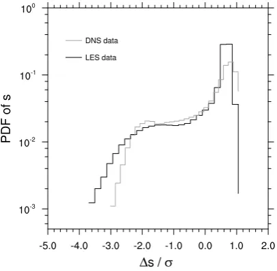
Fig. 2. PDF ofs from LES data of DYCOMS and from a DNS study. Both PDFs are calculated at a height level close to the cloud top where the variance of horizontal winds are at their respective maximum. The DNS data corresponds to a local study of turbu-lent mixing at cloud top, due solely to evaporative cooling (Mellado et al., 2010).
Using a double-Gaussian distribution, the PDF ofsis writ-ten as
P (s)=aP1(s)+(1−a)P2(s)
=√a
2π σ1
exp −1
2
s−s
1 σ1
2!
+√1−a
2π σ2
exp −1
2
s−s
2
σ2
2!
, (2)
whereP1andP2are single-Gaussian distributions ands1, s2,σ1andσ2are the mean and the standard deviation of the two single-Gaussian distributions. The relative weightsaand (1−a)can be interpreted as the corresponding area fractions (see Appendix). By convention and without loss of general-ity, we chooses1> s2. With five parameters to determine the PDF, the double-Gaussian distribution is highly flexible on the one hand. On the other hand, operational NWP models or GCMs are not able to predict five moments of the distri-bution ofs. Therefore closure assumptions will have to be chosen carefully (see Sect. 3.2).
In order to be able to analyse the LES data and the observational data in terms of the closure equations, we next aim to find the best fit of a double-Gaussian distribution to the PDF of s for each level of our LES data set and each five-minute interval in the observational data set. Because the skewness of the distribution is a crucial parameter in our closure, we establish an additional constraint for the fit which retains the skewness of the given PDF for the fitted
double-Gaussian distribution. Instead of varying the five parameters of the double-Gaussian distribution (a,s1,s2,σ1, σ2) like Larson et al. (2001a) did, we expresss1as a function ofa,s2,σ1,σ2and the mean, the standard deviation and the skewness of the given PDF,s,σ andsk, using the definition of the third standardized moment of a double-Gaussian distribution: sk=a
3s1−s
σ σ1 σ 2 +
s1−s
σ
3
+
(1−a)
3s2−s
σ
σ2
σ
2
+s2−s
σ
3
(Lewellen and Yoh, 1993; Larson et al., 2001a).
The values ofs,σ andskare obtained from the LES data or the observational data to evaluate the above equation and hence four parameters are left to be fitted (a,s2,σ1,σ2). To calculate the best skewness-retaining fit for each level of the LES data and each five-minute interval in the observational data set, we first doχ2-tests in the relevant region of the pa-rameter space. Because this procedure gets computationally expensive easily (at least if four parameters are to be fitted like it is done here), we only search for a coarse estimation of the best fit for the four parameters and then use this best fit as input for the Nelder–Mead downhill simplex method (Press et al., 1992) to find the actual minimum. In Fig. 1 two examples of the distribution ofsin a cloud layer of the LES data, one with positive skewness and one with negative skew-ness, are shown together with their best skewness-retaining double-Gaussian fit.
3.2 Closure equations
Even if we assume that the first three moments of the PDF ofsare readily available from an NWP model or a GCM, for example, from a higher-order closure boundary layer model, the number of parameters has to be reduced from five to three, that is, two closure equations are necessary. Larson et al. (2001a) suggested
σ1
σ =1+γ sk
√
α+sk2, σ2
σ =1−γ sk
√
α+sk2 (3) withα=2.0 andγ=0.6 ands1> s2by convention.
Analysing the different LES cases by fitting a double-Gaussian distribution to the (normalized) PDF ofsfor each vertical level as described in Sect. 3.1, we obtainσ1/σ and σ2/σ and plot them as a function ofsk (Fig. 3a and b). It is noted that high σ1/σ or σ2/σ values (>1.5) at sk=0 are an artifact of a double-Gaussian distribution being fit-ted to a distribution that is not skewed. In this case a single-Gaussian distribution might represent the given distribution well. So ifa approaches 0.0 (or 1.0) during the fitting pro-cedure, the second (or first) single-Gaussian distribution of the double-Gaussian distribution might fit the given distribu-tion so well that the terminadistribu-tion criteria for the fitting pro-cedure is reached, independent of the shape of the first (or second) single-Gaussian distribution which is essentially ir-relevant because of its small amplitude. Therefore, forsk=0
1646 A. K. Naumann et al.: A refined statistical cloud closure
Fig. 2.
PDF of
s
from LES data of DYCOMS and from a DNS study. Both PDFs are calculated at a height level
close to the cloud top where the variance of horizontal winds are at their respective maximum. The DNS data
corresponds to a local study of turbulent mixing at cloud top, due solely to evaporative cooling (Mellado et al.,
2010).
a) LES data for
σ
1b) LES data for
σ
2c) observational data for
σ
1Fig. 3.
LES data of ARM, ASTEX, RICO and DYCOMS and observational data from the RICO campaign
along with the closure equations from Larson et al. (2001a) (dashed line) and the new closure equations (solid
line). Note that the new closure equations are fitted to the LES data of RICO and DYCOMS rather than to all
available case studies. The grey shading in (c) corresponds to two times the standard deviation from the four
LES cases in (a). The legend in (a) also applies to (b).
26
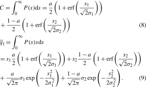
Fig. 3. LES data of ARM, ASTEX, RICO and DYCOMS and observational data from the RICO campaign along with the closure equations
from Larson et al. (2001a) (dashed line) and the new closure equations (solid line). Note that the new closure equations are fitted to the LES data of RICO and DYCOMS rather than to all available case studies. The grey shading in (c) corresponds to two times the standard deviation from the four LES cases in (a). The legend in (a) also applies to (b).
particularly high or low values ofσ1/σ orσ2/σ can be ig-nored, when evaluating the closure equations.
Because we defineds1> s2, large values for σ1/σ repre-sent the cloudy tail in shallow cumulus, wheresk has high positive values. In stratocumulus, where the skewness is neg-ative, large values forσ2/σ represent the non-cloudy part of the cloud layer. Larson et al. (2001a) analysed observational data from the ASTEX campaign and found only very few measurements of high positive skewness. They therefore sug-gested an antisymmetric behaviour for σ1/σ andσ2/σ de-pending onsk(Fig. 3a and b). In contrast, we find from the different LES case studies that in the cumulus regimeσ1/σ has higher values thanσ2/σin the stratocumulus regime.
This broken antisymmetric behaviour is consistent with the physical understanding that cloudy updrafts in shallow cumulus are more vigorous than non-cloudy downdrafts in stratocumulus. For the shallow cumulus cloud cores the up-per limit is a moist adiabatic ascent, while the stratocumulus downdrafts are only initially cloudy and as soon as they be-come cloud-free follow a dry adiabatic descent. Because the downdrafts are not exactly the reversed process of the up-drafts, the tails of the PDFs ofsare different for both cloud regimes, that is, the tails are heavier in the cumulus regime than in the stratocumulus regime.
Using thes1> s2convention, we suggest a refinement of the parameterization of Larson et al. (2001a) using a modi-fied set of closure equations (Fig. 3a and b)
σ1 σ =
1+γ1√skα if sk >0 1+γ3√sk
α+sk2 if sk≤0 σ2
σ =
1−γ2√sk
α+sk2 if sk >0 1−γ4√sk
α+sk2 if sk≤0
(4)
withα=2.0 adopted from Larson et al. (2001a). Fitting the parametersγn with a simple least square fit to the LES data
sets of DYCOMS and RICO, we find best agreement for γ1=0.73,γ2=0.46,γ3=0.78 andγ4=0.73. By fitting the closure equations to only the two data sets of DYCOMS and RICO, which cover the stratocumulus and the cumulus type cloud regime, respectively, the LES data sets of ASTEX and ARM remain as independent test data sets. This generic di-vision in training and test data aims to permit a later com-parison between the error of this new parameterizations and other parameterizations from the literature (see Sect. 4). The main difference between this set of closure equations and the one from Larson et al. (2001a) is the dependence ofσ1/σ onskfor (large) positive values of skewness, that is, for the shallow cumulus regime.
Fig. 4. Bimodal PDF ofsfrom the RICO case at cloud base withsk= 0.04. While the LES data shows
a bimodal distribution and the double-Gaussian fit is able to capture this shape, the two parameterizations
coincide in assuming a single-Gaussian distribution for vanishing skewness. For further explanation of the
legend see Fig. 1.
27
Fig. 4. Bimodal PDF ofs from the RICO case at cloud base with sk=0.04. While the LES data shows a bimodal distribution and the double-Gaussian fit is able to capture this shape, the two pa-rameterizations coincide in assuming a single-Gaussian distribution for vanishing skewness. For further explanation of the legend see Fig. 1.
clouds (A. Schanot, personal communication, 2012) while with LES all stages of the life cycle of such clouds are mod-eled. Therefore in the observational data regions with partic-ularly highs are undersampled. Nevertheless, the few data points with high skewness obtained from observational data of the RICO campaign fit well into the range of values found from LES and align rather with the introduced closure equa-tions than with the ones from Larson et al. (2001a).
A difficulty in the parameterization of Larson et al. (2001a) as well as in the new parameterization is the treat-ment of distributions that are characterized bysk≈0. Both sets of closure equations are constructed such that atsk=0 the normalized standard deviations σ1/σ =σ2/σ=1, that is for the closure equations the double-Gaussian distribution collapses to a single-Gaussian distribution as the skewness vanishes. In the LES data in the range ofsk≈0, distributions that match a single-Gaussian distribution occur as well as bi-modal double-Gaussian distributions, where the two modes balance in a way that the skewness almost vanishes (Fig. 4). The latter distributions often appear in the cumulus regimes at cloud base and are characterized by σ1/σ≈σ2/σ <1 (Fig. 3). Though the bimodal distributions with zero skew-ness cannot be captured adequately by the closure equations, the induced error is relatively small and will be discussed again in Sect. 4.
Knowing the first three moments of the distribution of s for a certain model level, σ1 and σ2 can now be calculated via the closure equations (Eq. 4), while a, s1 and s2 are obtained from the definition of the first three moments of a double-Gaussian distribution
(Larson et al., 2001a, Eqs. 22–24 therein):
sk−
a(1−a)
1−aσ1 σ
2
−(1−a)σ2 σ
2
1 2
3σ1 σ
2
−3σ2 σ
2
+ 1−2a
a(1−a)
1−a
σ1
σ
2
−(1−a)
σ2
σ
2
=0 (5)
s1−s σ =
1−a
a
12
1−a
σ1
σ
2
−(1−a)
σ2 σ 2 1 2 (6) s2−s
σ = −
a
1−a
12
1−aσ1 σ
2
−(1−a)σ2 σ 2 1 2 , (7) where Eq. (5) may be solved numerically for a. Alterna-tively, to avoid an iterative solution for a more computational efficient implementation in a GCM or an NWP model, an (e.g., polynomial or matched asymptotics) approximation of a as a function ofskcan be used. For the present analysis however, we solve fora numerically using a simple bisec-tion method with an accuracy of 10−6which typically took about 30 iterations.
Comparing the parameterized distribution ofsto the orig-inal LES data in all four case studies (Fig. 1, ASTEX and ARM not shown), we find that the new parameterization is able to represent the differences in the distribution ofs in a shallow cumulus regime as well as a stratocumulus regime and therefore represents the tails in a shallow cumulus regime better than the parameterization by Larson et al. (2001a).
Having determined a double-Gaussian PDF ofs, the cloud fraction,C, and the average liquid water of a large-scale grid box,ql, are found by integration:
C=
Z ∞
0
P (s)ds=a
2
1+erf
s
1 √
2σ1
+1−a
2
1+erf
s2 √ 2σ2 (8)
ql=
Z ∞
0
P (s)sds
=s1 a 2
1+erf
s
1 √
2σ1
+s2 1−a
2
1+erf
s
2 √
2σ2
+√a
2πσ1exp
− s 2 1 2σ12
!
+1√−a
2πσ2exp
− s 2 2 2σ22
!
. (9)
Note that for the introduced parameterization the normal-ized parameters of the double-Gaussian PDF (a,(s1−s)/σ, (s2−s)/σ,σ1/σ,σ2/σ) only depend onsk(Eqs. 4–7). There-fore withQ1≈s/σ, Eqs. (8) and (9) can be rearranged such that C and the normalized average liquid water, ql/σ, are functions ofskandQ1only.
1648 A. K. Naumann et al.: A refined statistical cloud closure
3.3 Parameterization of the liquid water flux
In contrast to the cloud fraction and the average liquid water, the liquid water flux cannot be found analytically by taking onlysinto account, but it also depends on the vertical veloc-ity,w. Instead of using a joint PDF ofsandw, we are here heading for a more straightforward way following Cuijpers and Bechtold (1995). They determined the liquid water flux, w0q0
l, from the flux ofs,w0s0, by w0q0
l =F Cw0s0, (10)
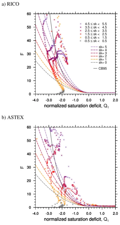
whereCis the cloud fraction.F is a proportionality constant that forC <1.0 can be interpreted as a measure of which part of the joint PDF ofw0ands0is found in the cloudy part of the domain. Therefore, limC→1.0F=1.0. Using coarse resolu-tion LES data of shallow cumulus and stratocumulus cases, Cuijpers and Bechtold (1995) found a dependence ofF on the normalized saturation deficit,Q1, andskwith the depen-dence onskmost notable near cloud base whereskis close to zero. Nevertheless, they suggest thatF is described fairly well as a function ofQ1only, givingF =exp(−1.4Q1)for Q1≤0 andF =1.0 forQ1>0.
Using Eq. (10), we find from the different LES cases a dependence of F on both Q1 and sk (Fig. 5, ARM and DYCOMS not shown). Using our training data sets (RICO, Fig. 5a, and DYCOMS), we propose
F =
(
aexp(b sk)Q21+1 if Q1≤0
1.0 if Q1>0
(11)
witha=1.5 andb=0.25 for a new parameterization. The proposed parameterization seems to be appropriate also for the testing data sets (ARM and ASTEX, Fig. 5b). Because this new parameterization is too sensitive to high sk for Q1<−4.0 and therefore gives unreasonable values at a thin layer near cloud top, we limit their range of application to Q1≥ −4.0. We findQ1<−4.0 only in a thin layer at cloud top, where the liquid water flux is close to zero. A similar unreasonable behaviour is found for the parameterization of Cuijpers and Bechtold (1995) and we will therefore apply the same limit to both parameterizations when testing it in the following with LES data. In a GCM or an NWP model the cloud top behaviour is very sensitive to the interplay of the cloud parameterization and the boundary layer scheme. Therefore a meaningful validation of the cloud top behaviour should be done in such a model with all feedbacks present. However, as a first attemptw0q0
l=0 forQ1<−4.0 might be sufficient.
4 A priori testing of the cloud closure
Having introduced a new set of closure equations forσ1/σ, σ2/σ andF (Eq. 4 and Eq. 11, respectively), we now anal-yse the quality of the new parameterizations with a priori
a) RICO
, Q1
b) ASTEX
, Q1
Fig. 5. New parameterization of F (dashed lines) as a function of the normalized saturation deficit and the
skewness along with the parameterization of Cuijpers and Bechtold (1995, CB95) and the LES data (crosses).
28
Fig. 5. New parameterization ofF (dashed lines) as a function of the normalized saturation deficit and the skewness along with the parameterization of Cuijpers and Bechtold (1995, CB95) and the LES data (crosses).
testing in LES and by comparing the introduced parameteri-zations with parameteriparameteri-zations from the literature. Note that the usefulness of a priori testing is in the assessment of va-lidity and accuracy of the parameterizations assumptions (see e.g., Pope, 2000, p. 601). To decide which parameterization is most useful in a certain NWP model or GCM a comparison based on a posteriori testing has still to be done.
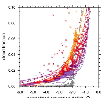
a) parameterization ofCby Larson et al. (2001a)
, Q1
b) new parameterization ofC
, Q1
c) parameterization ofqlby Larson et al. (2001a)
, Q1
d) new parameterization ofql
, Q1
Fig. 6.The parameterizations (dashed lines) as a function of the normalized saturation deficit and the skewness
shown together with the LES data of the ASTEX case (crosses).
29
Fig. 6. The parameterizations (dashed lines) as a function of the normalized saturation deficit and the skewness shown together with the LES
data of the ASTEX case (crosses).
(positiveskand negativeQ1) because the main differences between these two parameterizations are found for the cu-mulus regime. For stratocucu-mulus the two parameterizations differ only marginally.
For high positive skewness it is found that the new parame-terization reproduces the LES data better than the parameter-ization of Larson et al. (2001a) which overestimatesCandql for a givenQ1. Remember that zero skewness for the closure equations equals the case of a single-Gaussian distribution ofs (like assumed in Sommeria and Deardorff, 1977; Mel-lor, 1977), while in the LES data bimodal distributions occur as well. In this case and with increasing normalized satura-tion deficit (which at cloud base corresponds to increasing height), the parameterizations first overestimate and later un-derestimate the cloud fraction. For the normalized average liquid water the effect is less relevant (see also Fig. 7).
To give an estimate of the error of the different parameter-izations, the profiles ofC,qlandw0q0
l from the LES test data sets are compared with the results of the different parameter-izations (Fig. 7a, b and c). The new parameterization is able to reproduce the profiles ofC andql in the shallow cumu-lus layer better than the parameterization using the closure equations from Larson et al. (2001a). Both cloud schemes are clearly superior to a single-Gaussian cloud closure, which severely underestimatesqlandCand in particular is hardly able to diagnose any liquid water between cloud base and cloud top in the shallow cumulus layer. For the stratocumu-lus layer, the three parameterizations do not differ noticeably. A distinct difference between testing error (as in ASTEX; Fig. 7a and b) and training error (as in RICO; Fig. 7d and e) is not found.
For the profiles ofw0q0
l, Eq. (10) is used withF param-eterized like suggested for the new parameterization. For
1650 A. K. Naumann et al.: A refined statistical cloud closure
a)
C
in ASTEX
b)
q
lin ASTEX
c)
w
0q
0l
in ASTEX
d)
C
in RICO
e)
q
lin RICO
f)
w
0q
0l
in RICO
Fig. 7.
Profiles of cloud fraction, average liquid water and the liquid water flux from LES cases ASTEX (testing
dataset) after
25
h and RICO (training dataset) after
36
h of simulation. For the liquid water flux,
C
used in
Eq. (10) has either been taken from the original LES data (
C
LES) or from the new parameterization (
C
new).
The legend in (a) also applies to (b,d,e), the legend in (c) also applies to (f). Note the logarithmic scale on the
x-axis in (a) and (b).
30
Fig. 7. Profiles of cloud fraction, average liquid water and the liquid water flux from LES cases ASTEX (testing data set) after 25 h and
RICO (training data set) after 36 h of simulation. For the liquid water flux,Cused in Eq. (10) has either been taken from the original LES data (CLES) or from the new parameterization (Cnew). The legend in (a) also applies to (b, d, e), the legend in (c) also applies to (f). Note the logarithmic scale on thexaxis in (a) and (b).
comparison the parameterization by Cuijpers and Bechtold (1995) using an exponential fit ofF that only depends on Q1 is also shown in Fig. 7c for the ASTEX case. The new parameterization is able to reproduce the shape of the pro-files ofw0q0
las well as their absolute values. Again, for stra-tocumulus the two parameterization do not differ noticeably. To estimate the effect ofC in the new parameterization,C used in Eq. (10) has either been taken from the original LES data or from the new parameterization. It is shown thatC has a minor influence on the profile compared to the differ-ence between the two different parameterizations ofF. At the top of the cumulus layer for both the test data set ASTEX and the training data set RICO the new parameterization un-derestimatesw0q0
l. Note again that for a shallow layer with Q1<−4.0 at cloud top the parameterizations of the liquid water flux are not valid while the liquid water flux is close to zero.
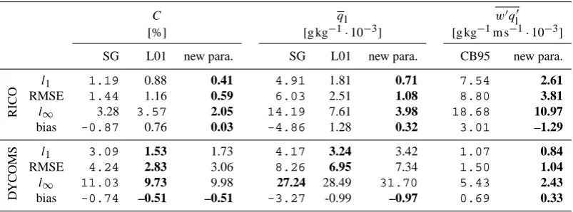
For a more quantitative analysis, the errors of the different parameterizations are summarized for the testing data sets in Table 2 and for the training data sets in Table 3. The dif-ferent error metrics used are the mean absolute error,l1, the root mean square error, RMSE, the maximum absolute er-ror,l∞and the bias. Their computation formulas are given in the caption of Table 2. For the cloud fraction and the av-erage liquid water, the proposed closure equations are fit to the LES data sets of RICO and DYCOMS. Therefore the new parameterization is optimized for RICO and DYCOMS and the error given for the new parameterization for those cases is a training error which is potentially lower than the error of an independent test data set. Nevertheless, we do not find a per-ceptible higher error for the test data sets ASTEX and ARM compared to the training data sets RICO and DYCOMS.
Table 2. Errors of the different parameterizations for the testing data sets, ASTEX and ARM.
C ql w0ql0
[%] [g kg−1·10−3] [g kg−1m s−1·10−3]
SG L01 new para. SG L01 new para. CB95 new para.
ASTEX
l1 1.10 0.66 0.41 2.37 1.21 0.72 3.39 2.43
RMSE 2.67 1.26 0.88 4.00 2.00 1.51 5.22 3.54
l∞ 19.70 9.31 7.05 23.12 10.73 10.98 19.11 11.44
bias –0.16 0.35 0.19 -1.22 0.82 0.42 -1.41 –0.83
ARM
l1 1.35 0.61 0.53 4.60 0.97 0.57 35.51 8.72
RMSE 1.85 0.84 0.87 6.67 1.42 1.15 42.10 11.78
l∞ 5.33 2.83 3.58 16.00 6.10 6.30 109.93 34.73
bias -1.21 0.30 –0.02 -4.43 –0.29 0.32 35.51 5.30
Parameterizations: SG – single Gaussian, L01 – Larson et al. (2001a), CB95 – Cuijpers and Bechtold (1995), new para. – new
parameterization. Error metrics:l1=1/nPni=0|1xi|, RMSE=(1/nPni=0(1xi)2)0.5,l∞=maxni=0|1xi|and bias=1/nPni=01xiwith 1xi=xpara.,i−xLES,i,x∈ [C, ql, w0q0l]andibeing a index for different vertical levels and output time steps. Values shown are averages over the last three output time steps of the LES data, where clouds are present, and over all vertical levels, where eitherxLES,iorxpara.,iare nonzero. To calculatew0q0
l para.,CLEShas been used in Eq. (10). Smallest errors are printed in bold, largest in typewriter. Note that the parameterizations ofw0ql0is only valid forQ1≥ −4.0, whileCandqlare calculated over the whole range ofQ1.
Table 3. Errors of the different parameterizations for the training data sets, RICO and DYCOMS.
C ql w0ql0
[%] [g kg−1·10−3] [g kg−1m s−1·10−3]
SG L01 new para. SG L01 new para. CB95 new para.
RICO
l1 1.19 0.88 0.41 4.91 1.81 0.71 7.54 2.61
RMSE 1.44 1.16 0.59 6.03 2.51 1.08 8.80 3.81
l∞ 3.28 3.57 2.05 14.19 7.61 3.98 18.68 10.97
bias -0.87 0.76 0.03 -4.86 1.28 0.32 3.01 –1.29
D
YCOMS
l1 3.09 1.53 1.73 4.17 3.24 3.42 1.07 0.84
RMSE 4.24 2.83 3.06 8.26 6.95 7.34 1.50 1.04
l∞ 11.03 9.73 9.98 27.24 28.49 31.70 5.43 2.43
bias -0.74 –0.51 –0.51 -3.27 -0.99 –0.97 0.69 0.33
For further description of the abbreviations and error measures please see Table 2.
Though the double-Gaussian parameterizations are restricted to their double-Gaussian families by the respective closure equations, both double-Gaussian families are able to repre-sent skewed distributions while a single-Gaussian distribu-tion is not skewed. Therefore the double-Gaussian families are able to represent both cumulus and stratocumulus. For stratocumulus the absolute values of skewness are less than for cumulus, therefore the difference in the errors between the single-Gaussian and the double-Gaussian parameteriza-tions is smaller.
Comparing the two parameterizations based on double-Gaussian distributions, the new parameterization matches the LES data better than the parameterization by Larson et al. (2001a) for ASTEX, whereas for ARM the two parameteri-zations have similar error magnitudes (Table 2). This is rea-sonable, because the closure equations have most notably been changed for high positive skewness which frequently
occurs in ASTEX but is rather scarce for ARM. The same effect can also be found in the training error (Table 3). While a lower error of the new parameterization compared to the er-ror of the parameterization of Larson et al. (2001a) is found for RICO (where high positive skewness occurs frequently), similar error magnitudes are found for DYCOMS (where the skewness is small).
For the liquid water flux, the error of the parameteriza-tion can be reduced distinctly by the new parameterizaparameteriza-tion compared to the parameterization of Cuijpers and Bechtold (1995). The new parameterization depends onQ1as well as onsk while the parameterization of Cuijpers and Bechtold (1995) is only dependent onQ1. The additional dependence of the new parameterization onskenables a more precise es-timation ofF which reduces the error in all four LES cases.
1652 A. K. Naumann et al.: A refined statistical cloud closure
5 Error dependence on domain size and the role of mesoscale structures
NWP models approach resolutions of only a few kilometers (e.g., Baldauf et al., 2011) which is considerably less than the domain sizes of all our LES cases. Hence, the question arises if the introduced PDF scheme is still applicable at such reso-lutions. We therefore investigate the dependence of the error of the new parameterizations on the domain size considered. To do so the domain of the four different RICO simulations has been divided into subdomains, the RMSE and the bias have been calculated in each subdomain and then averaged over all subdomains of the same size. These subdomains in our analysis of the LES data correspond to the grid spacing of an NWP or mesoscale model. The RICO simulations used differ in their overall domain size as well as in the initial hu-midity profiles of the simulations, giving “standard RICO” and “moist RICO” simulations (see Sect. 2.1.4).
For subdomain sizes smaller than 5 km, the RMSE in-creases rapidly with decreasing subdomain size for both standard and moist RICO simulations (Fig. 8). This rapid increase is probably due to the subdomain size approaching the size of individual cloud structures (i.e., larger cumulus clouds). When these two scales converge, the variability in-creases rapidly and a continuous, smooth distribution like the proposed family of double-Gaussian PDFs cannot appropri-ately represent the shapes of the subdomain PDFs. This re-sults in a larger spread of the LES data around the closure equations and consequently in an increasing RMSE with de-creasing subdomain size. The inde-creasing RMSE can be in-terpreted such that the PDF-based, deterministic scheme be-comes inappropriate at such small scales and one would have to use a stochastic approach instead.
With standard initial conditions, rain rates are small and no mesoscale structures develop, that is, the cloud field re-mains random. Then, for subdomain sizes larger than 10 km the RMSE is small, being around 0.005 and 0.001 g kg−1 for cloud fraction and liquid water, respectively. With moist initial conditions, precipitation appears more readily and mesoscale structures, that is, cloud streets, mesoscale arcs and cold pools, develop from 20 h onwards as discussed by Seifert and Heus (2013). In these moist cases and with subdomain sizes larger than 10 km, the cloud frac-tion as well as the liquid water are mostly overestimated by the double-Gaussian parameterization (positive bias). The RMSE amounts to about 0.017 and 0.04 g kg−1 for cloud fraction and liquid water, respectively, which for each vari-able corresponds to roughly 10 % of their respective max-imum values. With decreasing subdomain size the RMSE for the moist RICO simulations decreases until the subdo-main size reaches 5–10 km. At such subdosubdo-main sizes the RMSE is similar for standard and moist RICO simulations. For the moist RICO simulations and large subdomain sizes, the PDFs ofshave comparatively longer tails with few very high values of s. This different shape emerges from the
more localized but more intense convection and the large cloud free cold pool areas in the moist RICO case. The pa-rameterized double-Gaussian PDF, which is fitted to non-organized random cloud fields with small rain rates, is not able to capture the longer tails of the distributions ofs ad-equately. Therefore, for a given skewness the normalized varianceσ1/σis underestimated for moist RICO simulations with mesoscale structures.
The discussed error dependence on the domain size and the investigation of the moist RICO case show, on the one hand, that even with a perfect knowledge of the first three moments of the PDF ofsit remains challenging to construct a parameterization which is truly scale adaptive. On the other hand, the statistics of the cloud field at small scales seems to be independent enough from the mesoscale structures and higher rain rates to make the PDF scheme useful for a broader range of cloud regimes than the original LES data set used for the parameterization. Taking into account both the increas-ing error at very small subdomain sizes and the difficulties of the scheme to represent cloud properties in the moist RICO case, we conclude that the proposed scheme is most appro-priate for NWP models or GCMs with horizontal resolution of about 5–20 km.
For the liquid water flux, the new parameterization does not depend explicitly on a certain family of PDFs but the factorFis directly parameterized and depends onQ1andsk. With this parameterization the error of the liquid water flux seems to be less dependent on the development of mesoscale structures and higher rain rates, possibly because there is no direct dependence of the parameterization on the shape of the PDF ofs. A dependence of the error of the liquid water flux on the subdomain size is found in accordance with the error of the cloud fraction and average liquid water.
6 Extension to autoconversion rate
Autoconversion of cloud droplets to rain drops is a key process in the formation of precipitation in warm clouds. Besides the cloud fraction, the average liquid water and the liquid water flux discussed above, the autoconversion rate is another variable that depends among others on the variability of the liquid water mixing ratio (e.g., Pincus and Klein, 2000). In simple autoconversion schemes (e.g., Kessler, 1969; Sundqvist, 1978), other dependencies are ne-glected and the autoconversion rate only depends on the liq-uid water mixing ratio. With this simplification the autocon-version rate can also be handled by PDF-based schemes.
Following Kessler (1969, K69) and replacing the liquid water mixing ratio with the extended liquid water mixing ra-tio, the autoconversion rate,AK69, is given as
a) RMSE of
C
b) RMSE of
q
lc) RMSE of
w
0q
0l
d) bias of
C
e) bias of
q
lf) bias of
w
0q
0l
Fig. 8.
Dependence of the error of the parameterized cloud fraction, liquid water and liquid water flux on the
domain size. Shown are different simulations of the RICO case (average error over two output time steps after
24
h); in the moist RICO cases mesoscale structures develop, while in the standard cases the cloud field remains
random.
Fig. 9.
Profile of the autoconversion rate in ASTEX after
25
h of simulation. Note the logarithmic scale on
the x-axis. Notation: LES: autoconversion rate calculated using the full 3D-field of LES data, SG:
single-Gaussian parameterization, DG: double-single-Gaussian parameterization using the new closure equations, DG L01:
double-Gaussian parameterization using the closure equations from Larson et al. (2001a).
31
Fig. 8. Dependence of the error of the parameterized cloud fraction, liquid water and liquid water flux on the domain size. Shown are
different simulations of the RICO case (average error over two output time steps after 24 h); in the moist RICO cases mesoscale structures develop, while in the standard cases the cloud field remains random.
whereH is the Heaviside step function,scrit=0.5 g kg−1 is a critical threshold below which no autoconversion occurs andkis a rate constant set tok=10−3s−1.
Alternatively, Khairoutdinov and Kogan (2000, KK00) suggested a parameterization based on data from a single large-eddy simulation using spectral bin microphysics, that is, resolving the drop size distribution explicitly. They found that a good fit to the bulk autoconversion rate is
AKK00(s)=c1sc2H (s) (13) with c1=(5.829×10
6
Nc )
c2 and c
2=1.89. Within the factor c1, they introduced a dependence on the number of cloud droplets,Nc. Because Nc in UCLA-LES is assumed to be constant throughout a simulation,c1 can be treated as con-stant in this study.
For both autoconversion schemes, K69 and KK00, the domain-averaged autoconversion rate,A, is then found by integration over the PDF ofs:
Apara.=
Z ∞
s0
Apara.(s)P (s)ds (14)
with s0=scrit for Kessler (1969) and s0=0 g kg−1 for Khairoutdinov and Kogan (2000). While the integral can be
solved analytically for Kessler (1969), this is not possible for the scheme of Khairoutdinov and Kogan (2000) because the exponent ofs,c2, is not a natural number.
Seifert and Beheng (2001, SB01) derived an explicit equa-tion for the autoconversion rate which is formulated using Long’s piecewise polynomial collection kernel and a uni-versal function that is estimated by numerically solving the stochastic collection equation. Doing so they arrived at
ASB01=
kaukτρ0 N2
c
s4H (s) (15)
with kau=6.808×10¹⁸m3kg−1s−1 and kτ=1+(81−au(τ )τ )2. Here ρ0 is the base state density depending on height and 8au(τ ) is a universal function depending on the internal timescale,τ=1−ql/(ql+qr), designed to take into account the broadening of the droplet spectrum with time. Note that qris the rain water content which is not included inql. This dependence on the internal timescale makes it impossible to integrateASB01according to Eq. (14) as long as the PDF of τ is unknown in terms of the PDF ofswhich would require the use of a joint PDF or even the introduction of time cor-relations to the problem. Nevertheless, as the SB01 autocon-version rate is expected to give more realistic results than the
1654 A. K. Naumann et al.: A refined statistical cloud closure
simple autoconversion schemes described above, the SB01 autoconversion rate is used as a reference to be compared to the other autoconversion schemes. In our study the full 4-D field ofτis, of course, known from LES and a compensatory factor forkτ can be determined for each level and each time
step individually by solving
ALES(z, t ) (16)
=kτ,LES(z, t ) 1 (nx)2
kauρ0
Nc2
nx
X
i=1
nx
X
j=1
s4 xi, yj, z, tH (s)
for kτ,LES. Here nx is the number of LES grid boxes in each horizontal direction. Then the ability of the new double-Gaussian parameterization to be used in combination with the SB01 autoconversion rate can be tested usingkτ,LES: ASB01=kτ,LES(z, t )
kauρ0
N2
c
Z ∞
0
s4P (s)ds. (17) Note that for the use in an NWP model or a GCM,kτ,LES would have to be estimated by some other method and that kτ,LESis not equal to a horizontal mean ofkτ.
From Fig. 9 showing the different autoconversion rates for the ASTEX case, it is apparent that the profiles of the au-toconversion rate differ substantially both in shape and by several orders of magnitude in absolute value among the different parameterizations of the autoconversion rate (K69, KK00, SB01). While the single-Gaussian cloud closure only captures the stratocumulus type cloud layer around 2100 m, the new double-Gaussian cloud closure is additionally able to diagnose the autoconversion rate quite accurately for the cumulus layer. The same results hold for the other three LES cases (not shown).
Usingkτ,LESas described above, the new double-Gaussian cloud closure is able to reproduce the profile of the SB01 au-toconversion rate well for most heights. This is remarkable becauseASB01is proportional to the 4th moment ofswhich makesASB01especially sensitive to errors introduced by the cloud closure. Nevertheless, at the cloud top of the stratocu-mulus layer the new double-Gaussian cloud closure overes-timates the SB01 autoconversion rate. This overestimation might be related to the difficulties of LES in resolving the strong gradients that occur at a stratocumulus cloud top.
Using the closure equations of Larson et al. (2001a) (as it is done exemplary with the KK00 parameterization in Fig. 9) compared to using the new closure equations gives small and probably negligible differences in the cumulus layer.
Overall the double-Gaussian PDF scheme is successful in capturing the effect of the sub-grid variability on the autocon-version rate, which is crucial for the representation in the cu-mulus layer. Nevertheless, the uncertainty due to the choice of the autoconversion scheme itself remains. Especially the K69 scheme leads to a strong overestimation compared to KK00 and SB01, but also KK00 shows a much higher auto-conversion rate in the lowest part of the cumulus cloud layer compared to SB01.
a) RMSE ofC b) RMSE ofql c) RMSE ofw0q0
l
d) bias ofC e) bias ofql f) bias ofw0ql0
Fig. 8. Dependence of the error of the parameterized cloud fraction, liquid water and liquid water flux on the
domain size. Shown are different simulations of the RICO case (average error over two output time steps after
24h); in the moist RICO cases mesoscale structures develop, while in the standard cases the cloud field remains
random.
Fig. 9. Profile of the autoconversion rate in ASTEX after25h of simulation. Note the logarithmic scale on
the x-axis. Notation: LES: autoconversion rate calculated using the full 3D-field of LES data, SG:
single-Gaussian parameterization, DG: double-single-Gaussian parameterization using the new closure equations, DG L01:
double-Gaussian parameterization using the closure equations from Larson et al. (2001a).
31
Fig. 9. Profile of the autoconversion rate in ASTEX after 25 h
of simulation. Note the logarithmic scale on thexaxis. Notation: LES: autoconversion rate calculated using the full 3-D field of LES data, SG: single-Gaussian parameterization, DG: double-Gaussian parameterization using the new closure equations, DG L01: double-Gaussian parameterization using the closure equations from Larson et al. (2001a).
7 Conclusions
We introduce a refined statistical cloud closure using double-Gaussian PDFs. Following the work of Larson et al. (2001a), who provided an elegant framework for a diagnostic param-eterization of the cloud fraction and the average liquid water, we modified their parameterization especially in the case of strong positive skewness of the distribution of the extended liquid water mixing ratio, s, that is, for shallow cumulus clouds. The introduced double-Gaussian closure is based on different LES case studies and is supported by observational data from aircraft measurements in shallow cumulus. It is re-lying on the first three moments ofsas input parameters and is shown to be superior in diagnosing the cloud fraction and average liquid water profiles compared to a single-Gaussian approach that only needs the first two moments ofsfor input. A priori testing also suggests improved accuracy compared to existing double-Gaussian closures.
The dependence of the error of the parameterization on the domain size and the appearance of mesoscale structures has also been tested a priori with LES. Below a domain size of about 5 km the error of the parameterization of the cloud fraction, the average liquid water and the liquid water flux is increasing rapidly with decreasing domain size. If mesoscale structures occur that are accompanied by higher rain rates and the domain size is chosen large enough to include these mesoscale structures, the error of the parameterization of the cloud fraction and the liquid water is larger than without the occurrence of mesoscale structures. Considering the liquid water flux, the error of the parameterization seems to be in-sensitive to the occurrence of mesoscale structures.
Finally, the cloud scheme has been applied to diagnose the autoconversion rate. Using autoconversion schemes of dif-ferent complexity, the new parameterization is able to re-produce profiles of the autoconversion rate adequately. The differences between the various autoconversion schemes are much larger than the error introduced by the double-Gaussian closures.
As a next step, a posteriori testing of the introduced pa-rameterization in a NWP model or a GCM that diagnoses or predicts the first three moments ofs, for example, from a higher-order closure boundary layer model (Machulskaya and Mironov, 2013), is essential to decide which parameter-ization is most useful in the chosen NWP model or GCM. However, such a analysis is beyond the scope of this study and therefore left for further research.
Appendix A
Derivation of the assumed PDF
The distributionP (s)=PS(s)in Eq. (2) for a given region
(e.g., the LES domain) is a marginal of a joint PDF,PSI(s, i),
PS(s)=
Z
PSI(s, i)di . (A1)
The discrete random variableI, which is commonly used in turbulent flows to introduce conditional statistics (e.g., Pope, 2000), is defined to take different values in differ-ent subregions. As subregions we choose to distinguish be-tween thermal areas (I =1) and its well-mixed environment (I=2) in case of shallow cumulus or between the well-mixed environment (I=1) and downdrafts (I=2) in case of stratocumulus. Then the distribution ofIcan be written as PI(i)=aδ(i−1)+(1−a)δ(i−2), (A2)
whereδ is the Dirac delta function and a is the area frac-tion of the thermals in a shallow cumulus regime or the area fraction of the well-mixed environment in a stratocumulus regime.
For the joint PDF Bayes’ theorem gives
PSI(s, i)=PS|I(s|I=i) PI(i), (A3)
wherePS|I(s|I=i)is the conditional PDF ofsin the
sub-regioni. Inserting Eqs. (A2) and (A3) in Eq. (A1), we arrive at
PS(s)=
Z
PS|I(s|I=i) (aδ (i−1)+(1−a) δ (i−2))di
=aPS|I(s|I=1)+(1−a) PS|I(s|I =2)
=aP1(s)+(1−a) P2(s) . (A4) Assuming that the PDFs ofs in the subregions,P1 and P2, are Gaussian distributed, Eq. (A4) is equal to Eq. (2). Therefore, in the shallow cumulus regimea, the relative am-plitude of the two single-Gaussian distributions, can be di-rectly interpreted as the area fraction of the thermals while in the stratocumulus regime(1−a)is the area fraction of the downdrafts.
Acknowledgements. We are happy to thank Thijs Heus for provid-ing the LES data of the ARM case, Allen Scharnot for his advise while analysing the observational data set from RICO, Dmitrii Mironov and Ekaterina Machulskaya for beneficial discussion on the closure and its possible application in NWP, Robert Pincus for beneficial discussion on model selection and Cathy Hohenegger as well as two anonymous reviewers for helpful comments that improved this manuscript. The separation in training and test data was suggested by both reviewers. The observational data from RICO was provided by NCAR/EOL under sponsorship of the National Science Foundation (http://data.eol.ucar.edu). This research was carried out as part of the Hans-Ertel Centre for Weather Research. This research network of Universities, Research Institutes and the Deutscher Wetterdienst is funded by the BMVBS (Federal Ministry of Transport, Building and Urban Development).
The service charges for this open access publication have been covered by the Max Planck Society.
Edited by: K. Gierens
References
Albrecht, B. A., Bretherton, C. S., Johnson, D., Schubert, W. H., and Frisch, A. S.: The Atlantic stratocumulus transition experiment – ASTEX, Bull. Am. Met. Soc., 76, 889–903, 1995.
Baldauf, M., Seifert, A., Förstner, J., Majewski, D., Raschen-dorfer, M., and Reinhardt, T.: Operationl convective-scale nu-merical weather prediction with the COSMO model: Descrip-tion and sensitivities, Mon. Weather Rev., 139, 3887–3905, doi:10.1175/MWR-D-10-05013.1, 2011.
Bougeault, P.: Modeling the trade-wind cumulus boundary layer. Part I: Testing the ensemble cloud relations against numerical data, J. Atmos. Sci., 38, 2414–2428, 1982a.
Bougeault, P.: Cloud-ensemble relations based on the Gamma prob-ability distribution for the higher-order models of the planetary boundary layer, J. Atmos. Sci., 39, 2691–2700, 1982b.
Bretherton, C. S., Krueger, S. K., Wyant, M. C., Bechtold, P., van Meijgaard, E., and Teixeira, J.: A GCSS boundary-layer cloud model intercomparison study of the first ASTEX
1656 A. K. Naumann et al.: A refined statistical cloud closure
lagrangian experiment, Bound.-Lay. Meteorol., 93, 341–380, 1999.
Brown, A. R., Cederwall, R. T., Chlond, A., Duynkerke, P. G., Golaz, J.-C., Khairoutdinov, M., Lewellen, D. C., Lock, A. P., MacVean, M. K., Moeng, C.-H., Neggers, R. A. J., Siebesma, A. P., and Stevens, B.: Large-eddy sim-ulation of the diurnal cycle of shallow cumulus convec-tion over land, Quart. J. Roy. Met. Soc., 128, 1075–1093, doi:10.1256/003590002320373210, 2002.
Cuijpers, J. W. M. and Bechtold, P.: A simple parametrization of cloud water related variables for use in boundary layer models, J. Atmos. Sci., 52, 2486–2490, 1995.
Gryanik, V. M. and Hartmann, J.: A turbulence closure for the con-vective boundary layer based on a two-scale mass-flux approach, J. Atmos. Sci., 59, 2729–2744, 2002.
Gryanik, V. M., Hartmann, J., Raasch, S., and Schröter, M.: A re-finement of the Millionshchikov quasi-normality hypothesis for convective boundary layer turbulence, J. Atmos. Sci., 62, 2632– 2638, 2005.
Helfand, H. M. and Kalnay, E.: A model to determine open or closed cellular convection, J. Atmos. Sci., 40, 631–650, 1983.
Kessler, E.: On the distribution and continuity of water substance in atmospheric circulations, Meteor. Monogr. 32, Amer. Meteor. Soc., Boston, 1969.
Khairoutdinov, M. and Kogan, Y.: A new cloud physics parameteri-zation in a large-eddy simulation model of marine stratocumulus, Mon. Weather Rev., 128, 229–243, 2000.
Larson, V. E., Wood, R., Field, P., Golaz, J., Haar, T. H. V., and Cotton, W.: Small-scale and mesoscale variability of scalars in cloudy boundary layers: One-dimensional probability density functions, J. Atmos. Sci., 58, 1978–1994, 2001a.
Larson, V. E., Wood, R., Field, P., Golaz, J., Haar, T. H. V., and Cotton, W.: Systematic biases in the microphysics and thermody-namics of numerical models that ignore subgrid-scale variability, J. Atmos. Sci., 58, 1117–1128, 2001b.
Larson, V. E., Golaz, J., and Cotton, W.: Small-scale and mesoscale variability in cloudy boundary layers: Joint probability density functions, J. Atmos. Sci., 59, 3519–3539, 2002.
Lewellen, W. S. and Yoh, S.: Binormal model of ensemble partial cloudiness, J. Atmos. Sci., 50, 1228–1237, 1993.
Machulskaya, E. and Mironov, D.: Implementation of TKE-scalar variance mixing scheme into COSMO, COSMO newsletter, 13, 25–33, 2013.
Mellado, J. P., Stevens, B., Schmidt, H., and Peters, N.: Probability density functions in the cloud-top mixing layer, New J. Phys., 12, 085010, doi:10.1088/1367-2630/12/8/085010, 2010.
Mellor, G. L.: The Gaussian cloud model relations, J. Atmos. Sci., 34, 356–358, 1977.
Mironov, D.: Turbulence in the Lower Troposphere: Second-Order Closure and Mass-Flux Modelling Frameworks, in: In-terdisciplinary Aspects of Turbulence, edited by: Hillebrandt, W. and Kupka, F., 756, 1–61, Springer Berlin Heidelberg, doi:10.1007/978-3-540-78961-1_5, 2009.
Moeng, C.-H. and Rotunno, R.: Vertical-velocity skewness in the buoyancy-driven boundary layer, J. Atmos. Sci., 47, 1149–1162, 1990.
Neggers, R. A. J., Köhler, M., and Beljaars, A. C. M.: A dual mass flux framework for boundary layer convection, Part I: Transport, J. Atmos. Sci., 66, 1465–1487, 2009.
Perraud, E., Couvreux, F., Malardel, S., Lac, C., Masson, V., and Thouron, O.: Evaluation of statistical distributions for the parametrization of subgrid boundary-layer clouds, Bound.-Lay. Meteorol., 140, 263–294, doi:10.1007/s10546-011-9607-3, 2011.
Pincus, R. and Klein, S. A.: Unresolved spatial variability and mi-crophysical process rates in large-scale models, J. Geophys. Res., 105, 27059–27065, 2000.
Pope, S. B.: Turbulent flows, Cambridge Univ. Press, 2000. Press, W. H., Teukolsky, S. A., Vetterling, W. T., and Flannery, B. P.:
Numerical Recipes in FORTRAN, Cambridge University Press, Cambridge, 1992.
Quaas, J.: Evaluating the “critical relative humidity” as a measure of subgrid-scale variability of humidity in general circulation model cloud cover parameterizations using satellite data, J. Geo-phys. Res., 117, D09208, doi:10.1029/2012JD017495, 2012. Rauber, R. M., Stevens, B., Ochs, III, H. T., Knight, C., Albrecht,
B. A., Blyth, A. M., Fairall, C. W., Jensen, J. B., Lasher-Trapp, S. G., Mayol-Bracero, O. L., Vali, G., Anderson, J. R., Baker, B. A., Bandy, A. R., Burnet, E., Brenguier, J. L., Brewer, W. A., Brown, P. R. A., Chuang, P., Cotton, W. R., Girolamo, L. D., Geerts, B., Gerber, H., Goke, S., Gomes, L., Heikes, B. G., Hud-son, J. G., Kollias, P., LawHud-son, R. P., Krueger, S. K., Lenschow, D. H., Nuijens, L., O’Sullivan, D. W., Rilling, R. A., Rogers, D. C., Siebesma, A. P., Snodgrass, E., Stith, J. L., Thorn-ton, D. C., Tucker, S., Twohy, C. H., and Zuidema, P.: Rain in shallow cumulus over the ocean – The RICO campaign, Bull. Am. Met. Soc., 88, 1912–1924, doi:10.1175/BAMS-88-12-1912, 2007.
Rotstayn, L. D.: On the “tuning” of autoconversion parameteriza-tions in climate models, J. Geophys. Res., 105, 15495–15507, 2000.
Seifert, A. and Beheng, K. D.: A double-moment parameterization for simulating autoconversion, accretion and selfcollection, At-mos. Res., 59-60, 265–281, 2001.
Seifert, A. and Heus, T.: Large-eddy simulation of organized pre-cipitating trade wind cumulus clouds, Atmos. Chem. Phys., 13, 5631–5645, doi:10.5194/acp-13-5631-2013, 2013.
Slingo, J. M.: The development and verification of a cloud predic-tion scheme for the ECMWF model, Q. J. R. Meteorol. Soc., 113, 899–927, 1987.
Smagorinsky, J.: On the dynamical prediction of large-scale con-densation by numerical methods, in: Physics of Precipitation, no. 5 in Geophys. Mon., 71–78, American Geophysical Union, Washington, USA, 1960.
Sommeria, G. and Deardorff, J. W.: Subgrid-scale condensation in models of nonprecipitating clouds, J. Atmos. Sci., 34, 344–355, 1977.
Stevens, B.: On the growth of layers of non-precipitating cumulus convection, J. Atmos. Sci., 64, 2916–2931, 2007.
Stevens, B. and Seifert, A.: Understanding macrophysical outcomes of microphysical choices in simluations of shallow cumulus con-vection, J. Met. Soc. Jap., 86, 143–162, 2008.
Stevens, B., Lenschow, D., Vali, G., Gerber, H., Bandy, A., Blomquist, B., Brenguier, J., Bretherton, C., Burnet, F., Campos, T., et al.: Dynamics and chemistry of marine stratocumulus – DYCOMS-II, Bull. Am. Met. Soc., 84, 579–594, 2003. Stevens, B., Moeng, C., Ackerman, A., Bretherton, C., Chlond,