www.geosci-model-dev.net/9/2999/2016/ doi:10.5194/gmd-9-2999-2016
© Author(s) 2016. CC Attribution 3.0 License.
Constraining a land-surface model with multiple observations by
application of the MPI-Carbon Cycle Data Assimilation System V1.0
Gregor J. Schürmann1, Thomas Kaminski2,a, Christoph Köstler1, Nuno Carvalhais1, Michael Voßbeck2,a, Jens Kattge1, Ralf Giering3, Christian Rödenbeck1, Martin Heimann1, and Sönke Zaehle1,4
1Max Planck Institute for Biogeochemistry, Hans-Knöll-Str. 10, 07745, Jena, Germany 2The Inversion Lab, Hamburg, Germany
3FastOpt, Hamburg, Germany
4Michel Stifel Centre Jena for Data-driven and Simulation Science, Jena, Germany apreviously at: FastOpt, Hamburg, Germany
Correspondence to:Gregor J. Schürmann ([email protected]) and Sönke Zaehle ([email protected]) Received: 30 November 2015 – Published in Geosci. Model Dev. Discuss.: 19 January 2016
Revised: 2 August 2016 – Accepted: 3 August 2016 – Published: 2 September 2016
Abstract.We describe the Max Planck Institute Carbon Cy-cle Data Assimilation System (MPI-CCDAS) built around the tangent-linear version of the JSBACH land-surface scheme, which is part of the MPI-Earth System Model v1. The simulated phenology and net land carbon balance were constrained by globally distributed observations of the frac-tion of absorbed photosynthetically active radiafrac-tion (FAPAR, using the TIP-FAPAR product) and atmospheric CO2 at a global set of monitoring stations for the years 2005 to 2009. When constrained by FAPAR observations alone, the system successfully, and computationally efficiently, improved sim-ulated growing-season average FAPAR, as well as its sea-sonality in the northern extra-tropics. When constrained by atmospheric CO2 observations alone, global net and gross carbon fluxes were improved, despite a tendency of the sys-tem to underestimate tropical productivity. Assimilating both data streams jointly allowed the MPI-CCDAS to match both observations (TIP-FAPAR and atmospheric CO2) equally well as the single data stream assimilation cases, thereby increasing the overall appropriateness of the simulated bio-sphere dynamics and underlying parameter values. Our study thus demonstrates the value of multiple-data-stream assimi-lation for the simuassimi-lation of terrestrial biosphere dynamics. It further highlights the potential role of remote sensing data, here the TIP-FAPAR product, in stabilising the strongly un-derdetermined atmospheric inversion problem posed by at-mospheric transport and CO2 observations alone. Notwith-standing these advances, the constraint of the observations on
regional gross and net CO2flux patterns on the MPI-CCDAS is limited through the coarse-scale parametrisation of the bio-sphere model. We expect improvement through a refined ini-tialisation strategy and inclusion of further biosphere obser-vations as constraints.
1 Introduction
Estimates of the net carbon balance of the terrestrial bio-sphere are highly uncertain, because the net balance cannot be directly observed at large spatial scales (Le Quéré et al., 2015). Studies aiming to quantify the contemporary global carbon cycle therefore either infer the terrestrial carbon bud-get as a residual of the arguably better constrained other com-ponents of the global carbon budget (Le Quéré et al., 2015) or rely on measurements of atmospheric CO2and the inversion of its atmospheric transport (Gurney et al., 2002). Both ap-proaches have the caveat that they are not able to provide ac-curate estimates at high spatial resolution, and cannot utilise the broader set of Earth system observations that provide in-formation on terrestrial carbon-cycle dynamics (Luo et al., 2012). Furthermore, they are diagnostic by nature, and there-fore lack any prognostic capacity.
can – in principle – benefit from the broader set of Earth system observations. However, studies comparing different land-surface models show a large spread of estimates of the seasonal and annual net land–atmosphere carbon exchange and their trends (Piao et al., 2013; Sitch et al., 2015). This uncertainty is one of the primary causes of discrepancies in future projections of stand-alone terrestrial biosphere models (Sitch et al., 2008) and coupled carbon-cycle climate models (Anav et al., 2013; Friedlingstein et al., 2014) for the 21st century. Next to the uncertainty due to different climate forc-ing (Jung et al., 2007; Dalmonech et al., 2015) and alterna-tive model formulations (Sitch et al., 2015), the uncertainty about the parameter values of the mathematical representa-tion of key carbon-cycle processes in these models are an important source of the model spread (Knorr and Heimann, 2001; Zaehle et al., 2005; Booth et al., 2012). This parametric uncertainty can be as large as the differences between mod-els. The spread among models limits our ability to provide further constraints of the net terrestrial carbon uptake.
A potential route to reduce parameter and process-formulation related uncertainties in the estimates of the ter-restrial carbon cycle is to systematically integrate the in-creasing wealth of globally distributed carbon-cycle obser-vations into models through data assimilation methods. A broad overview of potential observations and methodolog-ical choices is given in Raupach et al. (2005). Since com-putational run time is an important limiting factor in global carbon-cycle data assimilation, the development of a rel-atively “fast” but comprehensive system is advantageous. Knorr and Kattge (2005) investigated the use of a Monte Carlo approach for data assimilation with global models. They suggested that the computational burden (i.e. the run time) is too large to allow its application with a comprehen-sive land-surface model and an appropriate number of pa-rameters in the optimisation. Nevertheless, the method has been successfully applied at global scales for a reduced set of parameters and limited process representations (Ziehn et al., 2012). A computationally more efficient method is the use of gradient-based methods. For instance, approximating the gradient with finite differences, Saito et al. (2014) performed data assimilation of several data streams with the VISIT model.
An alternative to the finite difference method is to calcu-late the gradient precisely by a tangent-linear or adjoint ver-sion of the biosphere model. A prototype of such a carbon-cycle data assimilation system (CCDAS) based on an ad-vanced variational data assimilation scheme and a prog-nostic terrestrial carbon flux model (BETHY; Knorr, 1997, 2000) has demonstrated the potential to effectively con-strain the simulated carbon cycle with observations of atmo-spheric CO2(BETHY-CCDAS; Rayner et al., 2005; Scholze et al., 2007; Kaminski et al., 2013). Conceptually similar sys-tems have been built for other, more complex, global bio-sphere models. Applications of these alternative systems in-clude, for example, constraining the phenology of the JULES
model with the MODIS collection five-leaf area index prod-uct (Luke, 2011) and carbon fluxes in the ORCHIDEE model using observations from several FLUXNET sites (Kuppel et al., 2012, 2013). Previous studies with these systems fo-cussed on the effect of different (in situ and satellite) FAPAR observations at selected sites on simulated phenology with the ORCHIDEE model (e.g. Bacour et al., 2015) or on the joint use of site-level carbon flux and FAPAR observations (Kato et al., 2013). At the global scale, Forkel et al. (2014) investigated the use of long-term FAPAR data to constrain long-term trends in vegetation greenness simulated by the LPJmL model, whereas Kaminski et al. (2012) focussed on the joint assimilation of FAPAR and atmospheric CO2 obser-vations.
Here, we present the development and first application of a variational data assimilation system (Max Planck Insti-tute Carbon Cycle Data Assimilation System: MPI-CCDAS) built around the tangent-linear representation of the JSBACH land-surface model (Raddatz et al., 2007). JSBACH is a fur-ther development of the BETHY model, providing a more detailed treatment of carbon turnover and storage in the ter-restrial biosphere, as well as more detailed treatment of land-surface biophysics (Roeckner et al., 2003) and land hydrol-ogy (Hagemann and Stacke, 2014). JSBACH serves as a land-surface scheme to the MPI-Earth System Model (MPI-ESM; Giorgetta et al., 2013). Our objective with this devel-opment is twofold: (i) to improve the scope of the original BETHY-CCDAS by including a larger set of terrestrial cesses affecting the terrestrial carbon cycle; and (ii) to pro-vide a means to constrain the land carbon-cycle projections of JSBACH with several data streams, and thereby poten-tially also that of the MPI-ESM. Dalmonech et al. (2015) have shown that the simulated phenology, and its seasonal and interannual climate sensitivity, as well as the simulated seasonal net land–atmosphere carbon flux are reasonably ro-bust against climate biases in the MPI-ESM. One can there-fore expect that improvements of these aspects made with the MPI-CCDAS driven by observed meteorology will be main-tained in the coupled Earth system model.
2 Description of the MPI-CCDAS 2.1 The CCDAS method
The MPI-CCDAS applies a variational data assimilation ap-proach to estimate a set of model parameters and initial states given a range of observations. The variational data assimila-tion method is described in detail by Kaminski et al. (2013). In the following, we thus only give a brief overview of the method. The values and uncertainties for model parameter values, observations and the model are detailed in the fol-lowing sub-sections.
To take account of the uncertainty inherent in the descrip-tion of observed and simulated variables, the method op-erates on probability density functions (PDFs) and is con-veniently formulated in a Gaussian framework. The MPI-CCDAS uses the combined information provided by the model M(p) and the observations d to update the PDF describing the prior state of information on the model’s process-related parameters and initial state variables, com-bined in the model’s control vector p. This prior control vector is described by the mean ppr and the covariance of its uncertaintyCpr. The CCDAS method seeks to minimise the misfit between observed and modelled quantities by min-imising the cost functionJ:
J (p)=1
2(M(p)−d)
TC−1
d (M(p)−d)
+ p−pprT
C−pr1 p−ppr
,
(1)
whereCd is the covariance of combined uncertainty in the observations (with meand) and model simulation. The min-imum ofJ, denoted as the posterior control vectorppo, cor-responds to the maximum likelihood estimate.ppo thus bal-ances the misfit between modelled quantities and their ob-servational counterparts over the entire assimilation window, while taking independent prior information on the control vector into account. In other words, the vector d contains all observations used in the assimilation procedure, which act simultaneously to constrain the control vector. In con-trast to sequential assimilation schemes, the approach ap-plied here determines a model trajectory through the state space, which, in particular, ensures conservation of mass and energy (Kaminski and Mathieu, 2016).
Technically,J is minimised by a quasi-Newton approach with so-called Broyden–Fletcher–Goldfarb–Shanno updates of the Hessian approximation, in the implementation pro-vided by the numerical recipes (Press et al., 1992, dfpmin routine). The iterative procedure requires the gradient ∂J∂p , which is evaluated by the so-called tangent-linear version of the model. This tangent-linear model was generated by means of the Transformation of Algorithms in Fortran com-piler tool (TAF, Giering and Kaminski, 1998) through auto-matic differentiation (Griewank, 1989). This procedure re-gards the model code that evaluatesJ (p)as the composition
of a sequence of (very many) elementary operations (such as “+”, or “exp”) to which it applies the chain rule of calculus. Being implementations of the chain rule, the derivatives pro-vided by the tangent-linear code are as accurate as possible on a computer, i.e. up to machine precision. This contrasts the traditional numerical differentiation approach, which de-rives derivative approximations through a series of perturbed model runs (for example, so-called finite difference or di-vided difference approximations).
2.2 The forward model
The model that is optimised within the MPI-CCDAS is the JSBACH land-surface model (Raddatz et al., 2007; Brovkin et al., 2009; Reick et al., 2013; Schneck et al., 2013; Dal-monech and Zaehle, 2013). The model considers 10 plant functional types (PFTs: see Table 1). These PFTs are allowed to co-occur within a grid cell on separate tiles, but nonethe-less share a common water storage. Compared to the afore-mentioned JSBACH studies, the MPI-CCDAS does not use land-use change and land-use transition or dynamic vegeta-tion, but uses a multi-layer soil hydrology scheme (Hage-mann and Stacke, 2014). Appendix A gives a detailed de-scription of the relevant parts of JSBACH. The model is typ-ically used within the MPI-ESM (Giorgetta et al., 2013) and calculates the terrestrial storage of energy, water and carbon and its half-hourly exchanges between the atmosphere and the land surface. JSBACH is applied here uncoupled from the atmosphere and forced with reconstructed meteorology (see Sect. 2.6).
The application of gradient-based minimisation proce-dures is facilitated by a differentiable calculation ofJ (p). According the chain rule, this ultimately requires all code parts of the forward model that depend on the control vari-ables and impact the cost function to be differentiable. To improve differentiability, the original phenology scheme that describes the timing and amount of foliar area based on lo-gistic growth functions (Lasslop, 2011) was replaced by an alternative scheme developed explicitly for the needs of dif-ferentiable codes (Knorr et al., 2010, Appendix A1). Some further minor modifications were necessary to make the code differentiable. These changes included replacing look-up ta-bles with their continuous formulations, avoiding division by zero in the derivative code (e.g. through differentiation of
√
0 in the forward mode leading to√1
0in the differentiated code), and reformulating minimum and maximum calculations to allow a smooth transition at the edge. These modifications alter the calculations. However, they were implemented such that the differences in the modelled results compared to the original code are minimal.
2.3 The atmospheric transport model
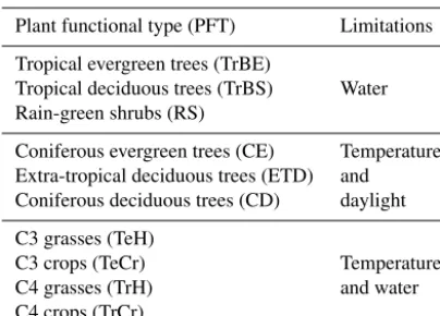
frac-Table 1.Plant functional types (PFTs) in the JSBACH model and the limitations that control the phenological behaviour of the re-spective PFT.
Plant functional type (PFT) Limitations
Tropical evergreen trees (TrBE)
Tropical deciduous trees (TrBS) Water
Rain-green shrubs (RS)
Coniferous evergreen trees (CE) Temperature
Extra-tropical deciduous trees (ETD) and
Coniferous deciduous trees (CD) daylight
C3 grasses (TeH)
C3 crops (TeCr) Temperature
C4 grasses (TrH) and water
C4 crops (TrCr)
tion, the computation of atmospheric transport is required, which is done here by transport model TM3 (Heimann and Körner, 2003). Specifically, we compute the response of monthly mean CO2mole fractionscto monthly mean surface fluxes f (extending 2 years back in time). Since the atmo-spheric transport of CO2is linear in the fluxes, the transport process can be written as
1c=M·f, (2)
whereM represents the TM3 responses as a transport ma-trix (Rödenbeck et al., 2003). For our analysis, we used the Jacobian representation of the TM3 model, version 3.7.24 (Rödenbeck et al., 2003), with a spatial resolution of about 4◦×5◦ (the “fine” grid of TM3), driven by interannually
varying wind fields of the NCEP reanalysis (Kalnay et al., 1996). The net exchange f is the sum of the terrestrial fluxes computed by JSBACH and those not computed by JS-BACH, i.e. prescribed ocean and fossil fuel fluxes (Sect. 2.5). Biomass burning fluxes are not explicitly included (see also the discussion in Sect. 4.5). During the assimilation of atmo-spheric CO2, any information on these latter fluxes in the ob-servations are consequently mapped to the respiratory fluxes simulated by JSBACH.
In the MPI-CCDAS, the atmospheric CO2mole fraction at the monitoring stations at the beginning of this simula-tion is specified as a globally constant offset COoffset2 , one of the parameters to be estimated. The resulting CO2mole fractions can then be directly compared with observed atmo-spheric CO2. Limiting the system to one global modifier was motivated by limitation in the computational run time, while an inclusion of an offset depending on the observation loca-tions could be easily implemented. With a spin-up of 2 years for the atmospheric transport, we allow the system to build up the latitudinal gradient of CO2. After the second year, there is no visible trend in the difference of observed CO2at Mauna Loa and the South Pole, leading us to conclude that 2 years are sufficient to spin up the atmosphere.
2.4 Model parameters
For this study, JSBACH parameters related to the phenol-ogy, photosynthesis and land carbon turnover (including ini-tial carbon stocks) were optimised (see Appendix A for a detailed model description). The default prior value and as-sumed prior Gaussian uncertainty of each parameter and the posterior values from the assimilation experiments are given in Table 2. The choice of these parameters was based on an extensive parameter sensitivity study on a much larger set of parameters across multiple biomes (Schürmann, unpub-lished results). We retained those parameters, for which we found a significant effect on modelled FAPAR and net CO2 exchange. In principle, it is possible to add more parameters, which are decisive for other modelled quantities such as soil moisture, and which might feed back to our observables. A brief explanation of the parameters involved in this study is given in the following.
The parameters controlling phenology (3max,τl,τw,Tφ,
tc, andξ) are allowed to take different values for each plant
functional type with the exception of ξ, which is a glob-ally valid parameter. While3max controls the LAI,ξ con-trols the rate of leaf growth, andτl is the timescale of leaf senescence.Tφandtcare temperature and day-length
thresh-olds, respectively, controlling the onset and end of vegetation activity. The parameterτw controls the shedding of leaves in response to phenology for drought-deciduous PFTs. Soil moisture in JSBACH follows a five-layer scheme (Hagemann and Stacke, 2014) and is coupled to vegetation processes via the phenology and the photosynthesis by influencing actual stomatal conductance and thus evapotranspiration.
The phenological parameter prior values and uncertainties are taken from Knorr et al. (2010), with the following three exceptions: the water control parameterτwrequired an adap-tation to account for the different soil-water formulations in the MPI-ESM compared to BETHY.τlfor the coniferous ev-ergreen PFT (CE) has also been adapted after preliminary site-scale studies to allow more flexibility in the seasonal-ity of the evergreen phenology (Schürmann, unpublished re-sults). Finally,3maxis left to its default JSBACH parameter value for all PFTs, with the exception of the coniferous ever-green PFT. For CE, a value of3max=1.7 m2m−2has been used, because preliminary model tests revealed a large bias in modelled FAPAR in CE-dominated regions, which adversely affected the model results of the carbon cycle.
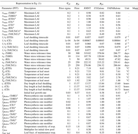
Table 2.Model parameters used in the data assimilation procedure with their prior and posterior values for the different assimilation
ex-periments. Parameters marked with∗represent scalars that are multiplied with their respective value in the model, given in Table D1. The
mapping variants are explained in Appendix C: (1) no lower bound; and (2) a lower bound at 0 for those parameters that are not allowed to take negative values.
Representation in Eq. (1): Cpr ppr ppo
Parameter (PFT) Description Prior sigma Prior JOINT CO2alone FAPARalone Unit Mapping
3max(TrBE)∗ Maximum LAI 0.2 1 0.98 0.82 0.84 . 2
3max(TrBD)∗ Maximum LAI 0.2 1 0.58 0.55 0.63 . 2
3max(ETD)∗ Maximum LAI 0.2 1 0.98 1.04 1.44 . 2
3max(CE)∗ Maximum LAI 0.2 1 1.00 0.84 1.01 . 2
3max(CD)∗ Maximum LAI 0.2 1 0.64 1.31 0.56 . 2
3max(RS)∗ Maximum LAI 0.2 1 1.33 0.94 1.24 . 2
3max(TeH,TeCr)∗ Maximum LAI 0.1 1 0.63 0.53 0.61 . 2
3max(TrH,TrCr)∗ Maximum LAI 0.1 1 0.53 0.49 0.59 . 2
1/τl(ETD) Leaf shedding timescale 0.01 0.07 0.057 0.057 0.079 d−1 2
1/τl(CE) Leaf shedding timescale 1e-04 5e-04 0.00067 0.00045 0.00064 d−1 2 1/τl(CD) Leaf shedding timescale 0.01 0.07 0.068 0.07 0.068 d−1 2
1/τl(TeH,TeCr) Leaf shedding timescale 0.01 0.07 0.098 0.076 0.079 d−1 2 1/τl(TrH,TrCr) Leaf shedding timescale 0.01 0.07 0.077 0.07 0.07 d−1 2
τw(TrBE) Water stress tolerance time 30 300 319.82 378.04 286.77 days 2
τw(TrBD) Water stress tolerance time 10 114 107.78 120.84 106.29 days 2
τw(RS) Water stress tolerance time 5 50 49.51 50.02 47.82 days 2
τw(TeH,TeCr) Water stress tolerance time 25 250 222.32 215.22 230.41 days 2
τw(TrH,TrCr) Water stress tolerance time 25 250 276.06 236.32 286.64 days 2
Tφ(ETD) Temperature at leaf onset 1 9.21 7.19 8.63 2.28 ◦C 1 Tφ(CE) Temperature at leaf onset 1 9.21 7.53 9.01 7.61 ◦C 1
Tφ(CD) Temperature at leaf onset 1 9.21 0.10 5.53 0.30 ◦C 1 Tφ(TeH,TeCr) Temperature at leaf onset 0.5 1.92 3.82 2.67 2.78 ◦C 1
Tφ(TrH,TrCr) Temperature at leaf onset 0.5 1.92 2.50 1.57 1.88 ◦C 1 tc(ETD) Day length at leaf shedding 1 13.37 13.57 13.84 13.60 hours 2 tc(CE) Day length at leaf shedding 1 13.37 14.22 13.69 14.12 hours 2
tc(CD) Day length at leaf shedding 1 13.37 14.94 13.66 14.73 hours 2 ξ Initial leaf growth rate 0.03 0.37 0.41 0.38 0.43 d−1 2
fphotos(TrBE)∗ Photosynthesis rate modifier 0.1 1 0.75 1.02 0.91 . 2
fphotos(TrBD)∗ Photosynthesis rate modifier 0.1 1 1.07 1.08 0.97 . 2
fphotos(ETD)∗ Photosynthesis rate modifier 0.02 1 0.99 1.00 1.00 . 2
fphotos(CE)∗ Photosynthesis rate modifier 0.03 1 0.95 1.00 1.00 . 2
fphotos(CD)∗ Photosynthesis rate modifier 0.06 1 1.04 1.05 1.00 . 2
fphotos(RS)∗ Photosynthesis rate modifier 0.1 1 1.01 1.05 1.00 . 2
fphotos(TeH)∗ Photosynthesis rate modifier 0.1 1 0.96 1.01 0.99 . 2
fphotos(TeCr)∗ Photosynthesis rate modifier 0.1 1 0.67 0.86 1.00 . 2
fphotos(TrH)∗ Photosynthesis rate modifier 0.1 1 1.04 1.02 1.06 . 2
fphotos(TrCr)∗ Photosynthesis rate modifier 0.1 1 0.87 0.94 1.00 . 2
Q10 Temperature sensitivity of resp. 0.15 1.8 1.90 1.81 1.80 . 2
fslow Multiplier for initial slow pool 0.1 1 0.50 0.51 1.00 . 2
2007). Thus, we introduce a single scaling coefficientfphotos:
V cmax=V cpriormax ·fphotos, (3)
Jmax=Jmaxprior·fphotos. (4)
Prior parameter ranges for each PFT were derived from the TRY database (Kattge et al., 2011).
Autotrophic respiration (Ra) in JSBACH follows Knorr (2000), who assumed that growth respiration is a fixed frac-tion (20 %) of the net assimilafrac-tion. Maintenance respira-tion scales with dark respirarespira-tion (with a parameterfaut_leaf), and thus V cmax, assuming that it is mainly driven by the amount of available photosynthates. The net primary produc-tion (NPP, the difference of GPP and Ra) is allocated to ei-ther a green or woody pool. Upon senescence, these pools turn over into three litter pools (above ground green, be-low ground green and woody) with PFT- and pool-specific turnover times. Heterotrophic respiration (Rh) of these pools responds to temperature according to aQ10formulation (see Appendix A).
Prior sensitivity studies have revealed that the most in-fluential parameters controlling carbon storage on land and the partitioning between autotrophic and heterotrophic res-piration were the leaf fraction of maintenance resres-piration (faut_leaf) and temperature response (Q10) of the carbon pools, which were both included as parameters into the opti-misation. The uncertainty of these parameters has been esti-mated based on the works of Mahecha et al. (2010) forQ10 and Knorr (2000) forfaut_leaf.
To account for non-steady-state conditions of the net car-bon flux at the beginning of the assimilation period, we fol-lowed the approach of Carvalhais et al. (2008) by estimating a global scaling factor for the size of the initial slow pool fslow. The inclusion offslowin the optimised parameters al-lows for the modification of global heterotrophic respiration and thereby adjusts the CO2growth rate by altering the net carbon flux to the atmosphere. However, the limitation of this approach is that it does not change the spatial distribution of carbon pools, which remains entirely controlled by the prior parameter values.
For this first application of the MPI-CCDAS, the most slowly varying pool has been selected (i.e. the soil carbon pool with a turnover time of 100 years). The initial condi-tions of other carbon pools were not included in the control vector to avoid the associated increase in the computational burden (e.g. run time). This consequently includes the risk of assigning any misrepresentation of modelled pool sizes to the soil carbon pool, and the changes in the carbon pool sizes after the assimilation should be interpreted with care. The uncertainty of fslowhas been set to 10 %, reflecting a mod-erate deviation from equilibrium (but see also the discussion in Sect. 4.4). The turnover-time parameters (see Eq. A18) were not included in the control vector, because their impact on land carbon fluxes was small compared to other
parame-ters (Schürmann, unpublished results) at the timescale of the MPI-CCDAS (a couple of years).
To account for minor offsets of the MPI-CCDAS with re-spect to the initial carbon content of the atmosphere, one sin-gle offset value COoffset2 is included in the set of estimated pa-rameters (see Sect. 2.3). COoffset2 was assumed to not deviate more than a few ppm, and its uncertainty was set accordingly. Uncertainties of all parameters were assumed to be Gaus-sian and exposed to the assimilation procedure in a form nor-malised by their prior uncertainty. In order to prevent param-eters from attaining physically impossible, negative values, some parameters were constrained at the lower end of the distribution to zero (see Table 2 and Appendix C).
2.5 Observational constraints and observation operators
2.5.1 Atmospheric CO2
Observed atmospheric CO2 mole fractions were obtained from the flask data/continuous measurements provided by different institutions (e.g. flask data of NOAA/CMDL’s sam-pling network, update of Conway et al., 1994, Japan Meteo-rological Agency, JMA, MeteoMeteo-rological Service of Canada, MSC, and many others; see Rödenbeck et al., 2003). Stations were selected in order to cover the global latitudinal gradient (Table B1), focussing on remote locations with little imprint of local fluxes. For cross-evaluation, an independent set of available station data was used (Table B2). The temporal res-olution of the CO2 original data at the monitoring stations (hourly to daily/weekly) depends on the specific station. The data were averaged to monthly means.
The MPI-CCDAS compares atmospheric CO2abundances at a monthly temporal resolution. In order to reduce the rep-resentation error, simulated CO2 abundances are only con-sidered at observational sampling times. The treatment of the observations of CO2 and their uncertainties follows Röden-beck et al. (2003). A floor value of 1 ppm is added to this un-certainty, similarly as in Rayner et al. (2005). Ancillary flux fields at monthly resolution were prescribed to represent the ocean (Jena CarboScope pCO2-based mixed layer scheme oc_v1.0 Rödenbeck et al., 2013) and fossil fuel (Emissions Database for Global Atmospheric Research EDGAR, Euro-pean Commission, Joint Research Centre , JRC) net CO2 fluxes.
2.5.2 TIP-FAPAR
explicitly designed to deliver products suitable for assimi-lation into climate and numerical weather prediction models. Similar schemes are implemented in most state-of-the-art ter-restrial biosphere models (e.g. Loew et al., 2014). The prod-uct used here was derived by running JRC-TIP on MODIS broadband visible and near-infrared white sky surface albedo input aggregated to the model grid separately for snow-free and snow-like background conditions in a similar way as de-scribed for the native 0.01 degree product (Pinty et al., 2011a, b; Clerici et al., 2010; Voßbeck et al., 2010).
Uncertainties in the FAPAR data are based on rigorous uncertainty propagation from the MODIS input albedos us-ing first and second derivative information (Voßbeck et al., 2010). A space and time invariant prior (except for the oc-currence of snow) is used, i.e. all spatio-temporal variability in the products is derived from the input products (including the MODIS snow flag). In contrast to alternative algorithms, there is no variability imposed through (possibly implicit) as-sumptions such as the distribution of land cover types (as in Knyazikhin et al., 1999), which avoids potential inconsisten-cies with the model’s own land cover (for more details see Disney et al., 2016). To reduce biases in the retrieved prod-ucts through the prior information, the prior is given a delib-erately low weight, which is aσ of 5 for the effective LAI (Pinty et al., 2011a).
We applied two filters to the global FAPAR product to ensure that potential model structural errors did not lead to compensating effects in the parameter estimation procedure and thus impede fitting the FAPAR data in other regions. First, owing to the fact that no specific crop phenology is im-plemented in JSBACH, grid cells with fractional crop cover-age of more than 20 % have been filtered out. A consequence of this filter is to mask the deciduous broadleaf PFT in the US and Europe, because in these areas, this PFT is collocated in crop-dominated pixels. Hence, the phenological parameters of the deciduous broadleaf PFT are only constrained by ob-servations from other locations – a fact that should be kept in mind when interpreting the deciduous broadleaf parame-ters. Second, grid points with correlations between the prior model and the observed FAPAR below 0.2 (i.e. prior phe-nology exhibits out-of-phase seasonal cycles) have also been filtered out. Together, these filters reduce the overall global coverage of the FAPAR constraint and thus the number of observations to be fitted (Fig. 1) by 57 %.
2.6 Experimental set-up
The MPI-CCDAS was driven by daily meteorological forc-ing (air temperature, specific air humidity, precipitation, downward short- and long wave radiation, wind speed) ob-tained from the WATCH forcing data set (Weedon et al., 2014). Annual CO2 mole fractions of the atmosphere as a forcing for the photosynthesis calculations of JSBACH were prescribed according to Sitch et al. (2015). Vegetation dis-tribution (Fig. E1) and other surface characteristics were
de-0.05 0.10 0.15 0.20 0.25 0.30 0.35
● ●
● ●
● ●
● ● ●
●
● ●
● ● ● ●
● ● ● ● ●
● ●
● ● ●
●
● ●●
● ● ●
●
● ●
● ●
● ● ●
● ●●
●
● ●●
● ●
● ● ● ● ● ● ●
Constraints ● Evaluation Constraints Evaluation
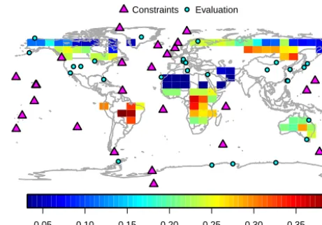
Figure 1.Location of the CO2observations (for constraining the
model and for evaluation) and the temporal median of the TIP-FAPAR uncertainties (given with the colour scale) in each pixel act-ing as a constraint.
rived from Pongratz et al. (2008). Although the MPI-CCDAS is flexible to be run at any spatial resolution, for computa-tional efficiency, it was applied at a coarse spatial resolution of about 8◦×10◦. Note that, as explained in Sect. 2.3, the atmospheric transport itself was simulated at 4◦×5◦.
Water and carbon-cycle state variables of JSBACH were initialised as follows: first, an equilibrium in terms of stores and long-term fluxes of water and carbon was achieved through repeated integration over the period 1979–1989 with corresponding meteorological forcing and atmospheric CO2 mole fractions of 1979. Starting from this equilibrium state, an integration followed with transient atmospheric and me-teorological forcing from 1979 to 2003 but with constant land cover. The final state of 2003 was then taken as the ini-tial condition for all MPI-CCDAS experiments. This spin-up procedure used the prior parameter values, i.e. it was not part of the assimilation loop for the parameter estimation.
We used the correlation, bias, root mean squared error and the Nash–Sutcliffe model efficiency (NSE) as evaluation statistics. NSE is defined as
NSE=1− P
i(di−mi)2
P
i di−di
2, (5)
where the indexidenotes individual pairs of observation (d) and model output (m) and an overbar the arithmetic mean. NSE=1 indicates a perfect model and for all NSE<0 the mean of the observations is a better predictor than the model itself.
Our study follows a factorial design to assess the benefit of each data stream, but also to evaluate the potential of as-similating more than one data stream and its effect on the carbon cycle: two experiments, each using one data stream alone as an observational constraint (CO2alone using only atmospheric CO2observations, and FAPARalone using only the TIP-FAPAR product), and one experiment using both data streams simultaneously as an observational constraint (JOINT), with each data stream equally weighted in the cost function (Eq. 1).
3 Results
3.1 Performance of the assimilation
The application of the MPI-CCDAS was successful within a feasible number (29 to 69) of iterations (with run times of 1 to 2 months), increasing from FAPARalone (using only TIP-FAPAR) to CO2alone (using only atmospheric CO2 ob-servations) and JOINT (using both observations simultane-ously; Table 3). For all three assimilation experiments, the value of the cost function was considerably reduced, while the posterior parameter values remained in physically plausi-ble ranges. Nevertheless, some parameter values (e.g.Tφof
the CD phenotype) deviated strongly from the prior values (Table 2). For FAPARalone, the value of the cost function was almost halved between the prior and the posterior run. Even stronger reductions of the cost function were obtained in the other two experiments using CO2as a constraint (Ta-ble 3).
Several statistics comparing the posterior model with ob-servations for FAPAR and CO2 (Tables 4 and 5) show that the model performance of the JOINT experiment was com-parable to the performance of the two single data-stream experiments relative to the assimilated quantity. The single data-stream assimilation experiments either showed no im-provement with respect to the other data stream (the fit of the CO2alone experiment to TIP-FAPAR), or even a degradation (the fit of the FAPARalone experiment to atmospheric CO2 observations). By contrast, the JOINT assimilation captured the main features of both data sources. Overall, these results suggest that both data streams can be successfully assimi-lated jointly with the MPI-CCDAS.
2007 2008 2009
0.0
0.2
0.4
0.6
0.8
Siberian FAPAR @ 59°, 120° (Lat, Lon)
Years
F
AP
AR
● ● ● ●● ●
● ●
● ●
● ● ● ●
●
● ●
● ● ●
●● ● ● ● ● ●
● ●
● ● ●●
●
●
● ●
● ● ● PRIOR CO2alone FAPARalone JOINT Obs
Figure 2.Example time series of FAPAR for an East Siberian pixel dominated by the CD-PFT to demonstrate the improvement in the timing of the phenology due to the data assimilation. TIP-FAPAR
observations are given with their mean (dots) and 1σuncertainties
(vertical lines).
During the assimilation procedure, the norm of the gradi-ent1 ∂J∂p (see Eq. 1) was considerably reduced by 3–4 orders of magnitude (Table 3). During the first tens of iterations of the assimilation procedure, the cost as well as the norm of the gradient were considerably reduced. In this initial phase of the assimilation, the parameter values also changed most strongly. However, some parameter values continue to change in later iterations without substantial reductions in the cost function or the norm of the gradient. The assimilation procedure finally stopped when the changes to the parame-ters became too small.
3.2 Phenology
The statistics of the comparison to the TIP-FAPAR data sets show an improvement of the model–data fit for all exper-iments relative to the prior model (Table 4). As expected, the improvement was strongest when using FAPAR (FA-PARalone and JOINT) as a constraint. One important rea-son for the improvement was a general reduction in mod-elled growing-season average FAPAR simulated by the MPI-CCDAS compared to the prior run. This decrease in FAPAR was mostly driven by a reduction of globally averaged foliar area of 0.41 m2m−2for the JOINT experiment (0.34 m2m−2 for FAPARalone and 0.59 m2m−2for CO2alone). Almost all PFTs contributed to the decrease in FAPAR, resulting from a reduction in the maximum leaf area index parameter (3max) for tropical deciduous forests, needleleaf deciduous forests, as well as herbaceous PFTs (crops and grasses). In addition, the water-stress parameterτw for drought-responsive PFTs played a secondary role in the leaf area reduction. The con-current increase in foliar area for extra-tropical deciduous and rain-green shrubs only plays a minor role in the model–
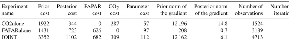
Table 3.Characteristics of the assimilation experiments. The prior and posterior cost-function values and the contribution of FAPAR, CO2 and the prior (second term in Eq. 1) to the posterior cost-function value are given, as well as the norm of the gradient, the number of observations acting as a constraint, and the number of iterations of the assimilation
Experiment Prior Posterior FAPAR CO2 Parameter Prior norm of Posterior norm Number of Number of
name cost cost cost cost cost the gradient of the gradient observations iterations
CO2alone 1922 344 0 287 57 12 196 14.8 1524 69
FAPARalone 1431 723 626 0 97 208 0.7 3189 29
JOINT 3352 1102 682 309 112 12 162 6.1 4713 69
0 1 2 3 4
JOINT
Temporal mean 2005‒2009 LAI [m2/m2]
−1.5 −1.0 −0.5 0.0 0.5 1.0 1.5
JOINT minus PRIOR
Temporal mean 2005‒2009
−1.5 −1.0 −0.5 0.0 0.5 1.0 1.5
JOINT minus CO2alone
Temporal mean 2005‒2009 LAI [m2/m2]
−1.5 −1.0 −0.5 0.0 0.5 1.0 1.5
JOINT minus FAPARalone
Temporal mean 2005‒2009
LAI [m2/m2] LAI [m2/m2]
Figure 3.Temporally averaged global LAI of the JOINT experiment and differences of the other experiments to the JOINT case.
data agreement, since these PFTs only cover a small fraction of the global land area.
In regions with a strong temperature control of phenology, the assimilation did not only change the average LAI during the growing season. Also, the timing of the onset and end of the growing season was improved, as demonstrated by the enhanced correlation and model efficiency of the MPI-CCDAS with respect to the TIP-FAPAR data (Table 4). This improvement was mostly the result of adjusting the param-eters Tφ and tc, which are the temperature and day-length
criteria determining when the vegetation switches from the
dormant to the active phase. In particular, the assimilation reduced the temperature control parameterTφ, which led to
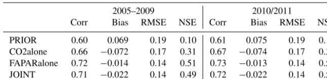
be-Table 4.Performance of the prior and posterior models compared with TIP-FAPAR observations (applying the same data quality screening as for the assimilation). The assimilation period (2005–2009) as well as a subsequent evaluation period (2010/2011) is shown. Abbreviations are Corr: correlation; Bias: Model – Observations; RMSE: Root mean squared error; NSE: Nash–Sutcliffe model efficiency.
2005–2009 2010/2011
Corr Bias RMSE NSE Corr Bias RMSE NSE
PRIOR 0.60 0.069 0.19 0.10 0.61 0.075 0.19 0.12
CO2alone 0.66 −0.072 0.17 0.31 0.67 −0.074 0.17 0.31
FAPARalone 0.72 −0.014 0.14 0.51 0.73 −0.013 0.14 0.52
JOINT 0.71 −0.022 0.14 0.49 0.72 −0.022 0.14 0.50
haviour of FAPAR. Notably, the CO2alone experiment also showed some improvement in the correlation and model ef-ficiency compared to TIP-FAPAR, although this experiment did not use the TIP-FAPAR data as a constraint. This sug-gests that the seasonal cycle of CO2bears some constraint on the timing of northern extra-tropical phenology.
The FAPARalone assimilation run performed best com-pared to TIP-FAPAR (Table 4). However, the JOINT exper-iment yielded a fairly similar (though not identical) perfor-mance with respect to the simulated FAPAR. The temporally averaged LAI demonstrates the overall similarity between the FAPARalone and JOINT experiments (Fig. 3). This sim-ilarity is also reflected in the parameter values of the phe-nology: the parameters of FAPARalone and JOINT were of-ten closer to each other than to CO2alone (Table 2). How-ever, in some cases, similar model performance was obtained with diverging model parameterisation: an example for this is the TrBE PFT, for which parameters of the JOINT and FAPARalone experiment were different, while the modelled foliar area was very similar. An explanation of this feature highlighting the potential benefits of multi-data-stream as-similation is given in Sect. 3.4.1. The most pronounced dif-ferences between the JOINT and FAPARalone experiments arose at locations where TIP-FAPAR data were not used as a constraint, such as crop-dominated pixels, in which the ETD PFT also covered a substantial part of the grid cell. These dif-ferences contributed strongly to the difdif-ferences in the glob-ally averaged foliar area.
Larger differences in simulated FAPAR occurred between the CO2alone and JOINT experiments (Table 4 and Fig. 3). The CO2alone experiment showed the smallest LAI, and thus the smallest FAPAR. This feature is especially pronounced in tropical regions, where the decrease was driven by the water-control parameter τw and the parameter controlling maximum foliar area 3max. The opposite pattern was ob-tained for the CD PFT, which showed a larger foliar area for CO2alone driven by an increased parameter3maxcompared to the other two experiments, in which foliar area and3max decreased. The likely explanation of this behaviour is given in Sect. 3.4.2.
3.3 Atmospheric CO2
The assimilation procedure strongly reduced the misfit be-tween the observed and modelled atmospheric mole fractions of CO2when using CO2as a constraint (CO2alone; Table 5). This was true for the seasonal cycle, the seasonal cycle’s am-plitude and the 5-year trend (Figs. 4 and 5). Conversely, the FAPARalone experiment showed a strong deterioration of the simulated atmospheric CO2 metrics compared to the prior model. Notwithstanding an improvement of the seasonal cy-cle amplitude of atmospheric CO2(Fig. 5), the 5-year trend of atmospheric CO2was much less conforming to the obser-vations, leading to a much faster increase in CO2 than ob-served (Table 5 and Fig. 4).
Introducing TIP-FAPAR as an additional constraint in the JOINT experiment did allow the MPI-CCDAS to match both the atmospheric CO2data and the TIP-FAPAR product: the simulated monthly CO2 mole fractions of the JOINT and CO2alone experiment are almost identical for most sites (Ta-ble 5 and Figs. 4 and 5).
The improvement of the simulated atmospheric CO2 for the CO2alone and JOINT assimilation runs persisted for the 2 years following the assimilation period, in which the model was run in a prognostic mode (driven by reconstructed me-teorology), with only minor degradation in model perfor-mance (Table 5). Both experiments clearly outperform the prior model, which is most obvious in the improvement of the NSE for the prognostic period.
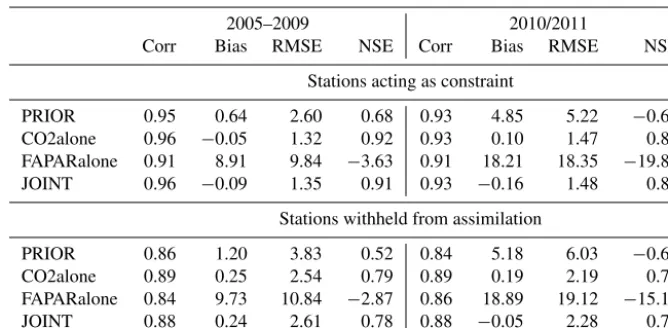
Table 5.Performance of the prior and posterior models compared with atmospheric CO2for constraining and evaluating sites and for the assimilation period (2005–2009) and the evaluation period (2010/2011). Abbreviations are Corr: correlation; Bias: model–observations; RMSE: root mean squared error; NSE: Nash–Sutcliffe model efficiency.
2005–2009 2010/2011
Corr Bias RMSE NSE Corr Bias RMSE NSE
Stations acting as constraint
PRIOR 0.95 0.64 2.60 0.68 0.93 4.85 5.22 −0.69
CO2alone 0.96 −0.05 1.32 0.92 0.93 0.10 1.47 0.87
FAPARalone 0.91 8.91 9.84 −3.63 0.91 18.21 18.35 −19.86
JOINT 0.96 −0.09 1.35 0.91 0.93 −0.16 1.48 0.87
Stations withheld from assimilation
PRIOR 0.86 1.20 3.83 0.52 0.84 5.18 6.03 −0.61
CO2alone 0.89 0.25 2.54 0.79 0.89 0.19 2.19 0.79
FAPARalone 0.84 9.73 10.84 −2.87 0.86 18.89 19.12 −15.14
JOINT 0.88 0.24 2.61 0.78 0.88 −0.05 2.28 0.77
3.3.1 Changes in carbon fluxes causing the changes in simulated CO2
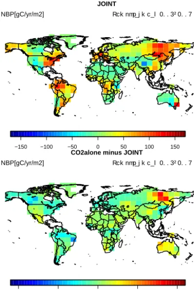
The changes in simulated atmospheric CO2 mole fractions originated from substantial changes of the seasonal ampli-tude and overall strength of the net carbon fluxes simulated by JSBACH. The application of the CO2constraint increased the global net biome production (NBP) from 1.0 Pg C yr−1 in the prior model to 3.2 Pg C yr−1 in the CO2alone and JOINT experiments. Conversely, using only TIP-FAPAR as a constraint decreased the NBP to −2.2 Pg C yr−1. In other words, using FAPAR data alone turned the biosphere into a net source (Table 6), inconsistent with current understanding of the global carbon cycle (Le Quéré et al., 2015).
Despite the similarity of the global NBP for the experi-ments with CO2as a constraint, the spatial patterns of NBP were different between the CO2alone and JOINT experi-ments (Fig. 6). The net uptake in both experiexperi-ments originated from boreal and tropical regions. However, the JOINT ex-periment showed an uptake in the boreal regions of conifer-ous evergreen and coniferconifer-ous deciduconifer-ous dominated pixels, whereas the net CO2 uptake in the CO2alone experiment was more concentrated on the coniferous deciduous regions. These differences will be further investigated in Sect. 3.4.2.
While the atmospheric observations constrained the net land–atmosphere CO2flux, the MPI-CCDAS model parame-ters act directly only on the gross carbon fluxes: gross pri-mary production (GPP), autotrophic respiration, and het-erotrophic respiration (Ra and Rh, respectively). Thus, the changes in simulated NBP were the indirect consequence of altered gross fluxes and land carbon pools. Although the globally integrated posterior GPP values were somewhat dif-ferent across the experiments (Table 6), the relative latitudi-nal patterns were fairly similar to each other (Fig. 7): a re-duction of GPP occurred globally, but was most prominent in tropical forests and grass/crop dominated regions in the
temperate and boreal zone. The GPP reduction was strongest for the CO2alone experiment and weakest (but still very pro-nounced) for FAPARalone. The generally reduced foliar area directly led to a reduced GPP of the terrestrial biosphere (in all experiments). The changes in the photosynthetic capac-ity (fphotos) (Table 2) often further reduced GPP. This was most pronounced for the crop and tropical evergreen PFTs (Table 2). In the JSBACH model, Ra is estimated as a direct function of canopy-integrated carboxylation capacity, which strongly correlates with GPP (Eq. A17). Simulated Ra and net primary production (NPP) thus quickly adjusted to the imposed change of GPP.
Application of the CO2 constraint in the CO2alone and JOINT experiment forced heterotrophic respiration (Rh) to be reduced to match the reduced NPP and the imposed atmo-spheric growth rate of CO2. The reduction in Rh was mainly driven by a reduction of the initial soil carbon pool (via the modifierfslow) to about 50 % of the prior value for the JOINT and CO2alone experiment (Table 6). Since the net carbon fluxes in the FAPARalone experiment were not constrained by the atmospheric CO2 observations, the assimilation did not adjust the heterotrophic respiration to balance the re-duced net primary productivity inre-duced from the altered FA-PAR. As a consequence, the net CO2flux to the atmosphere in the FAPARalone increased, leading to the overestimation of the growth rate of atmospheric CO2(Fig. 4).
3.4 Regional differences among the experiments
Table 6.Global averages of selected carbon-cycle components for the years 2005 to 2009 in PgC yr−1for fluxes and PgC for stocks and
comparison with independent estimates. Ra: autotrophic respiration. Rh: heterotrophic respiration. Reco: ecosystem respiration. NBP=GPP
−Reco=GPP−Ra−Rh=NPP−Rh. Vegetation carbon includes quickly overturning leaf and fine root carbon, as well as a woody
carbon pool.
PRIOR CO2alone FAPARalone JOINT Other estimates Other CCDAS
NPP 65.5 40.9 53.5 45.6 44–66a 40g
Ra 86.1 57.6 67.8 65.7
Rh 64.5 37.6 55.4 42.2
Reco 150.6 95.2 123.2 107.9
GPP 151.6 98.4 121.3 111.3 119±6b,123±8c 109–164h
NBP 1 3.2 −2.2 3.2 2.4±0.8d
Soil carbon 2649 1064.7 2187.1 1122.3 1343e
Vegetation carbon 424 388.5 420.5 407.3 442±146f
Litter carbon 239.9 189.8 212.8 193.9
aCramer et al. (1999); Saugier and Roy (2001);bJung et al. (2011);cBeer et al. (2010);dLe Quéré et al. (2015);
e http://webarchive.iiasa.ac.at/Research/LUC/External-World-soil-database/HTML/;fCarvalhais et al. (2014);gRayner et al. (2005);hKoffi
et al. (2012)
or by compensations between different parts of the globe (Sect. 3.4.2).
3.4.1 Tropics
The modelled foliar area in the tropics (dominated by the tropical evergreen PFT) was similar for the JOINT and FA-PARalone experiments (Fig. 3), but smaller for CO2alone. The simulated GPP of the JOINT experiment (Fig. 7) was somewhat lower than in the FAPARalone experiment, but still substantially larger than that of the CO2alone experi-ment. Notwithstanding these differences, the simulated net land–atmosphere CO2 exchange (Fig. 6) of the JOINT ex-periment was closer to the posterior estimate of CO2alone than to that of FAPARalone in terms of absolute values. This result was caused by compensating effects of the two obser-vational constraints (Fig. 8 and Table 2): the phenological parameters, notablyτw and3max, were substantially differ-ent between the FAPARalone and JOINT experimdiffer-ents, yet their modelled foliar area was very similar (Fig. 3). The rea-son for this was that the photosynthesis parameter modifier fphotos was reduced strongly in the JOINT experiment. This change caused the smaller GPP in the JOINT relative to the FAPARalone experiment. Through the effect of net photo-synthesis on canopy conductance (Eq. A14), the potential transpiration rate (Epot; Eq. A5) was strongly decreased. To-gether with the increase inτw (Eq. A5) in the JOINT exper-iment, the decline in Epothad the same effect on the simu-lated phenology as the smaller parameter changes in the FA-PARalone experiment. The lack of an FAPAR constraint in the CO2alone experiment allowed the assimilation to overly reduce the foliar area by increasing τw at the prior rate of photosynthesis and thusEpotto satisfy the constraint by the atmospheric CO2observations. As a consequence, due to the
water-cycle feedback, the modelled foliar area was clearly different between the JOINT and CO2alone experiments. 3.4.2 Boreal zone
The CO2alone and JOINT experiments showed simi-lar global statistics when compared with atmospheric CO2 observations (Table 5 and Fig. 4). Their global and hemispheric net carbon uptake was similar (North-ern Hemisphere: 2.24/2.20 PgC yr−1; Southern Hemisphere: 0.98/0.98 PgC yr−1), but their underlying spatial patterns were different, in particular in the boreal zone (Fig. 6). The entire boreal zone took up a large share of the global car-bon sequestration in the JOINT experiment (0.88 PgC yr−1), especially in coniferous deciduous (CD) dominated regions of Eastern Siberia (0.30 PgC yr−1). The CO2alone exper-iment showed a similar net carbon uptake in the boreal region, but the uptake in the CD dominated region was 0.16 PgC yr−1 stronger than in the JOINT experiment. This difference was mainly driven by larger foliar area and in-creased leaf-level productivity (parameterfphotos) of the CD PFT in the CO2alone experiment. In the same latitudinal band, coniferous evergreen trees showed reduced foliar area in the CO2alone experiment compared to the JOINT exper-iment, reducing the net uptake by 0.16 PgC yr−1, such that the differences in these regions cancel each other. These rel-atively small spatial differences do not prevent the posterior JOINT and CO2alone experiment from capturing the ampli-tude of the seasonal cycle at individual northern-most sta-tions.
pa-2005 2006 2007 2008 2009 2010 2011 2012 360 370 380 390 400 410 420
Summit, Greenland Observatory
0
C
O
2 mole fr
action [ppm] Evaluation ●● ● ● ● ● ● ● ● ● ● ●● ● ● ● ● ● ● ● ● ● ● ● ● ● ●● ● ● ● ●● ● ● ●● ● ● ● ● ● ● ●● ● ●● ●● ● ● ● ● ● ● ● ● ● ●● ● ● ● ● ● ● ● ● ● ●● ● ● ●● ● ● ● ●● ● ●● ● ●● ● ● ● ● ● ● ● ● ● ● ● ●● ● ● ● ● ● ● ● ● ●●● ●● ● ● ● ● ● ● ● ●●● ●● ● ● ● ● ● ●● ●● ●● ● ● ● ● ● ● ● ● ● ● ●●● ● ● ●● ● ● ● ●● ●● ● ● ● ●● ● ● ● ● ●● ● ● ● ● ● ● ● ● ● ●● ●●● ● ● ●● ● ● ● ● PRIOR CO2alone FAPARalone JOINT Observations
2005 2006 2007 2008 2009 2010 2011 2012
360 370 380 390 400 410 420
Alert, Nunavut (Canada)
0 C O2 mole fr action [ppm] Evaluation Constraining period ●● ●● ●● ● ●● ● ● ● ● ● ●● ● ● ● ●● ● ● ● ● ●● ● ● ● ● ● ● ● ● ●● ● ● ● ● ● ● ●● ● ● ● ●● ● ● ● ● ● ● ● ● ●● ● ●● ● ●● ● ● ● ● ● ●● ● ●● ● ● ● ●● ● ● ●● ● ● ● ● ● ● ● ● ● ● ● ● ●● ●● ● ● ● ● ● ● ● ●●● ●● ● ● ● ● ● ● ●●● ● ● ● ● ● ● ● ● ● ● ●●●●● ● ● ● ● ● ● ●● ● ●●● ● ● ● ● ● ● ● ● ● ● ●● ● ● ●● ● ● ● ●●● ●● ● ● ● ● ● ● ● ● ●●●● ● ● ●● ● ● ● ● PRIOR CO2alone FAPARalone JOINT Observations
2005 2006 2007 2008 2009 2010 2011 2012
360 370 380 390 400 410 420
Mauna Loa, Hawaii
C
O
2 mole fr
action [ppm] Evaluation Constraining period ●● ●● ● ● ●● ● ●● ●●● ●● ● ●● ● ● ●● ●● ● ●● ● ●● ● ● ●● ●●● ● ● ● ● ● ● ● ●● ●● ● ● ●● ● ● ● ● ●● ●● ● ● ●● ● ● ● ● ●● ●● ●●● ● ● ● ● ● ●● ●● ● ●● ● ●● ● ● ●● ● ● ● ● ●● ● ● ● ●● ● ● ● ● ● ●●● ● ● ●● ● ● ● ●● ●● ● ● ● ●● ● ● ● ● ● ●●● ● ● ●● ● ● ●●● ● ● ● ● ● ●● ● ● ●● ● ●●● ● ● ●● ● ● ● ● ● ●● ● ● ● ● ● ● ● ●● ● ●● ●● ● ● ● ● ● ● PRIOR CO2alone FAPARalone JOINT Observations
Figure 4. Time series of atmospheric CO2 as observed at
high-latitude evaluation site Summit and at two constraining sites, one at high latitudes (Alert) and one representative of the Northern Hemi-sphere (Mauna Loa) for the different prior and posterior models. The observations are given together with their uncertainty.
rameters cannot be adequately constrained by carbon-cycle observations from other parts of the globe. This relative scarceness of observations and independency of other re-gions allows the Eastern Siberian net carbon uptake to com-pensate for other regions’ fluxes in order to match the global growth rate. Additional observations would be required to al-low for spatially higher resolved estimation of the net fluxes.
4 Discussion
4.1 Comparison of the simulated carbon cycle with independent estimates
We have demonstrated that the JSBACH model is capable of reproducing the seasonal cycle and 5-year trend of the ob-served atmospheric CO2(Figs. 4 and 5, and Table 5). During the assimilation run, we have applied a careful selection of
0 5 10 15 20 25
Seasonal cycle amplitude of CO2 [ppm]
Latitude −90 −60 −30 0 30 60 90 ● ●● ●● ● ●● ● ● ● ●● ● ● ● ●● ● ● ● ●●● ● ● ●● ● ● ● ●●●● ● ●●● ● ● ●● ●● ● ●●● ● ● ●●●● ● ●●● ● ● ●● ● ● ● ●●●● ● ● ● ●● ● ●● ●● ● ● ● ● ● ● ●●● ● ● ●●● ● ● ●● ●● ● ●● ● ● ● ● ● ● ● ● ● ● ● ● ● ●●● ● ● ●● ● ● ● ●● ● ● ● ●● ●● ● ●●● ● ● ● ● ● ● PRIOR CO2alone FAPARalone JOINT Observation
Figure 5.Latitudinal distribution of atmospheric CO2seasonal
cy-cle amplitude, calculated as the difference between the maximum
and minimum CO2mole fractions of the averaged seasonal cycle of
the linearly de-trended signal from 2005 to 2009.
stations to avoid the impact of local sources on modelled at-mospheric CO2 mole fractions, which cannot be simulated with the current coarse resolution of the MPI-CCDAS. The evaluation at the cross-validation sites, which are located on land and thus closer to locally varying source patterns, also demonstrated a good skill of the posterior model for these sites. Overall, this does suggest that the improvement of the MPI-CCDAS’s ability to capture the observed CO2 dynam-ics at monthly to yearly timescales is reasonably robust. Our results further support earlier studies (Rayner et al., 1999; Kaminski et al., 1999; Peylin et al., 2013) that the observa-tional network of atmospheric CO2only constrains a limited number of spatio-temporal flux patterns.
−150 −100 −50 0 50 100 150
JOINT
Temporal mean 2005‒2009 NBP[gC/yr/m2]
−100 −50 0 50 100
CO2alone minus JOINT
Temporal mean 2005‒2009 NBP[gC/yr/m2]
Figure 6.Temporally averaged NBP of the JOINT assimilation, and the difference between the CO2alone and JOINT experiments.
in the northern extra-tropics between 30 and 60◦N, but to a
lower GPP in the tropical rain forests (Fig. 7). The reduction of GPP in the northern extra-tropics is likely associated with the overestimation of the seasonal cycle of atmospheric CO2 by the prior model, which was successfully reduced primar-ily by reducing northern extra-tropical productivity, in par-ticular in temperate and boreal grasslands. Nevertheless, our study supports earlier findings that despite some constraint on northern extra-tropical production, the constraint of ob-served atmospheric CO2on global production is small (Koffi et al., 2012).
A detailed comparison of the simulated vegetation and soil carbon stocks is beyond the scope of this paper, partly be-cause the simplifications of the spin-up procedure entail bi-ases in predicted vegetation and soil carbon stocks, as tran-sient land-use changes, forest management, and forest-age structure are ignored. It is nevertheless instructive to compare the simulated vegetation and soil carbon stocks to global to-tals from independent estimates to provide the context for the global carbon cycle simulated by MPI-CCDAS. The poste-rior experiments showed only little less carbon in vegetation (389–420 PgC) than the prior model (424 PgC; see Table 6). All of these estimates are lower than the 556 PgC vegeta-tion carbon based on updated Olson’s major world
ecosys-● ● ● ● ● ● ● ● ● ● ● ● ● ● ● ● ● ● ● ● ● ● ● ●
−50 0 50
0 5 10 15 20 Latitudinal distribution Latitude GPP [PgC y r − 1] ● ● ● ● ● ● ● ● ● ● ● ● ● ● ● ● ● ● ● ● ● ● ● ● ● ● ● ● ● ● ● ● ● ● ● ● ● ● ● ● ● ● ● ● ● ● ● ● ● ● ● ● ● ● ● ● ● ● ● ● ● ● ● ● ● ● ● ● ● ● ● ● ● ● ● ● ● ● ● ● ● ● ● ● ● ● ● ● ● ● ● ● ● ● ● ● ● ● ● ● ● ● ● ● ● ● ● ● ● ● ● ● ● ● ● ● ● ● ● ● PRIOR CO2alone FAPARalone JOINT Jung et al. (2011)
Figure 7.Latitudinal distribution of GPP for the prior and posterior models compared to the independent estimates of Jung et al. (2011).
tem carbon stocks2, but are comparable to a more recent es-timate of global vegetation carbon storage of 442±146 PgC (Carvalhais et al., 2014). The posterior amount of soil car-bon from the assimilation runs using atmospheric CO2as a constraint compare favourably (within the uncertainty) to the estimates of 1343 PgC based on the Harmonized World Soil Database (HWSD)3. This estimate is more appropriate for the presented comparison than the more recent and higher estimate of soil carbon by Carvalhais et al. (2014) of 1836– 3257 PgC (95 % confidence interval), as the latter includes estimates of permafrost carbon, which is not modelled with the current version of the MPI-CCDAS.
Our estimate of the net land carbon sink using atmo-spheric CO2as a constraint is slightly larger than the resid-ual land carbon sink estimate (without inclusion of land-use change fluxes) inferred from atmospheric measurements and auxiliary fluxes by Le Quéré et al. (2015), who derived a net uptake of 2.4±0.8 PgC yr−1 for the period 2000–2009. Correcting this estimate for the pre-industrial lateral carbon fluxes from land to the ocean via rivers would increase the terrestrial net land C uptake seen by the atmosphere (and thus the MPI-CCDAS) to 2.85 PgC yr−1; see Le Quéré et al., 2015 and Jacobson et al., 2007). Due to the interannual vari-ability of the land sink, the shorter time period of our sink estimate may have contributed to the difference between the estimates. However, it is more likely that the reason for the difference is the prescribed, comparatively small, net ocean carbon uptake of 1.1 PgC yr−1(Rödenbeck et al., 2013). This net ocean uptake applied in the MPI-CCDAS compares to the estimate of 2.4±0.5 PgC yr−1 of Le Quéré et al. (2015)4, which decreases to 1.95 PgC yr−1when correcting the
esti-2http://cdiac.ornl.gov/epubs/ndp/ndp017/ndp017b.html
3http://webarchive.iiasa.ac.at/Research/LUC/
External-World-soil-database/HTML/
4The estimates of Rödenbeck et al. (2013) and Le Quéré et al.
mate for the dissolved organic carbon (DOC) transport from land to oceans via river systems. Bearing in mind that the atmospheric CO2 observations more directly constrain the net global carbon fluxes at seasonal and annual scales rather than the gross land fluxes or land carbon pools, assuming a larger ocean net carbon uptake would have reduced the net land uptake simulated by MPI-CCDAS. Explicitly account-ing for DOC-based carbon losses from land in the JSBACH model would probably help to close the gap between the es-timates and thereby reduce the estimated land carbon storage inferred from the atmospheric data. Adding such a process formulation would thus permit the MPI-CCDAS to generate an estimate which is more compatible with that of Le Quéré et al. (2015).
4.2 Comparison to previous studies
Our results are consistent with earlier studies, which showed that JSBACH overestimates the seasonal cycle amplitude of atmospheric CO2(Dalmonech and Zaehle, 2013). The pos-terior estimates of this amplitude was considerably reduced, leading to an improved model performance in all three exper-iments (Fig. 5). This also holds for FAPARalone, for which the comparison with CO2is an independent evaluation. Note that the prior we reported here already relies on an adjusted 3maxparameter for the CE PFT (see Sect. 2.6). For the run with the off-the-shelf configuration of JSBACH as applied in Dalmonech and Zaehle (2013, results not shown), the high-latitude mean seasonal cycle amplitude was around 30 ppm, implying an overestimation of about 15 ppm. In the prior ex-periment including the adjusted 3maxfor the CE PFT, this overestimation was reduced to about 5–10 ppm. Applying only FAPAR as a constraint further reduced the overestima-tion of the high-latitude mean seasonal cycle amplitude (FA-PARalone experiment in Fig. 5). Adding CO2as a constraint further improves the fit to the seasonal cycle amplitude. In other words, boreal phenology, in particular maximum an-nual leaf area, has a considerable control on the seasonal cy-cle of the high-latitude atmospheric CO2signal. Using TIP-FAPAR helped to improve this metric of the carbon cycle despite the deterioration of the simulated longer-term CO2 trend (Fig. 4).
This conclusion is also supported by Kaminski et al. (2012), who constrained the BETHY-CCDAS jointly with at-mospheric CO2data and a different FAPAR product (Gobron et al., 2007). They found an improved seasonal cycle ampli-tude of CO2for their joint assimilation, which is in line with our findings. Through factorial uncertainty propagation with their assimilation scheme, Kaminski et al. (2012) also found that the inclusion of FAPAR yields only a moderate uncer-tainty reduction in the simulated carbon fluxes and mainly decreases the water flux uncertainties. Kaminski et al. (2012) therefore suggested that FAPAR only added little informa-tion to the modelled carbon cycle in addiinforma-tion to atmospheric CO2. In contrast, we have shown here a considerable impact
CO2alone JOINT FAPARalone
Parameter changes of TrBE
Multiple of pr
ior uncer
tainty
−3
−2
−1
0
1
2
3
Λmax τw fphotos
Figure 8.Parameter changes of tropical evergreen trees in multiples
of the prior uncertainty (asppoσ−ppr
pr ).
of the FAPAR data set by altering the spatial net carbon flux patterns between the JOINT and CO2alone experiments.
Our study showed considerable differences in the GPP es-timates, which were not reflected in the net carbon fluxes for the CO2alone and JOINT cases, as the net flux is more di-rectly constrained by the atmospheric CO2observations. Us-ing a variant of the BETHY-CCDAS, Koffi et al. (2012) also found large differences in their posterior GPP estimates rang-ing from 109 to 164 PgC yr−1resulting from the use of alter-native transport models, atmospheric station densities, and prior uncertainties. As in our study, their large GPP range was not reflected in large differences of the net land carbon flux. Our work thus supports earlier findings (Rayner et al., 2005; Scholze et al., 2007; Koffi et al., 2012) that despite some constraint on northern extra-tropical GPP, the global land GPP cannot be well constrained with atmospheric CO2 alone.
4.3 Discussion of the assimilation procedure
The results clearly show that two data streams can be successfully integrated with the MPI-CCDAS. The poste-rior parameter values (Table 2) were different between FA-PARalone and JOINT, as well as the CO2alone and JOINT experiments. This demonstrates that the joint use of the two data streams added information to the posterior parameter vector by preventing the degradation of the phenology sim-ulation when trying to fit the CO2 observations (Tables 5 and 4). This conclusion is also supported by the fact that the value of the cost function of the JOINT assimilation roughly equals the sum of the single-data-stream experiments, indi-cating consistency of the model with both data streams.
Hence, although the JSBACH phenology is only weakly influenced by the carbon-cycle component of JSBACH and mainly controlled by other drives (e.g. soil moisture, temper-ature), there are strong interactions among carbon and water cycle parameters and simulated FAPAR, a finding supported by Forkel et al. (2014). The combination of the two data streams in the JOINT experiment helped to keep parame-ters within acceptable bounds. The capability of assimilating multiple data streams simultaneously is a distinct advantage of the MPI-CCDAS over alternative strategies that assimilate multiple data streams following a sequential design of as-similating FAPAR prior to carbon-cycle information. An im-plementation of such a sequential assimilation likely reduces the number of parameters to be optimised in each step, and therefore allows a quicker solution of the optimisation prob-lem. However, this advantage comes at the cost of breaking the linkage between parameters, because side-effects of pa-rameter variations on other modelled quantities are ignored in the assimilation process. This can lead to simulation re-sults, in which the posteriori model of a sequential assimila-tion experiment will not match the observaassimila-tions equally well as obtained by simultaneous assimilation of the data streams. Since our results have demonstrated that a joint assimilation is feasible without impairing the fit to the individual data sources, a joint assimilation approach appears therefore rec-ommendable.
The assimilation procedure achieved a strong reduction of the cost function and the norm of the gradient (see Table 3). Although the relative reduction in the norm of the gradient was larger in the CO2cases than in the FAPARalone case, the norm did not not approach zero – contrary to the FA-PARalone case. Such a non-zero gradient was also noted by Rayner et al. (2005) in their CO2 assimilation with the BETHY-CCDAS. The fact that the MPI-CCDAS success-fully reduces the norm of the gradient for FAPAR suggests that this is not a general failure of the MPI-CCDAS but is specific to the particularities of the CO2set-up. It is presently unclear what is causing the assimilation to fail to reach the minimum of the cost function, warranting further investiga-tion of the non-linear nature and potential numerical issues regarding the computation of the gradient ∂J∂p (Eq. 1).
Fur-ther tests with alternative station network settings, parame-ter priors, or time periods for data assimilation will provide more insight into potential solutions to tackle this issue. Nev-ertheless, we believe that our results can still be meaningfully interpreted and used to evaluate the general capacity of the MPI-CCDAS as a comprehensive data assimilation tool. 4.4 Comments on the parameter set-up
The results presented in Sect. 3.2 show that there is a cer-tain degree of equifinality in the parameter values obcer-tained from the assimilation of TIP-FAPAR. This can happen when (i) certain parameters enter an insensitive regime where pa-rameter differences do hardly propagate to differences in the modelled foliar area, (ii) pixels are a composite of different plant functional types that can show compensating effects, and (iii) the atmospheric CO2 constraint imposes an addi-tional weight on changing FAPAR, because of the feedbacks through photosynthesis and stomatal conductance.
A cautionary note about the posterior parameter values is warranted: Some of the parameters of the JOINT and CO2alone experiment were altered strongly compared to the assumed prior uncertainty. This is possible within the MPI-CCDAS, because the prior contribution to the cost function is weak due to the small number of parameters compared to the number of observations. One example is thefslowparameter, which controls the initial soil carbon pool size and thus the disequilibrium between GPP and respiration (Table 2). An-other example is the photosynthesis parameterfphotosfor the tropical evergreen PFT in the JOINT experiment, which was reduced by more than 2.5 times the prior uncertainty and to roughly 75 % of its prior value. As a consequence, the assim-ilation procedure can result in parameter values with small prior probabilities. This either points toward too tight prior uncertainties, or to model structural problems.