www.geosci-model-dev.net/8/1763/2015/ doi:10.5194/gmd-8-1763-2015
© Author(s) 2015. CC Attribution 3.0 License.
Path-integral method for the source apportionment of
photochemical pollutants
A. M. Dunker
LLC, Bloomfield Hills, Michigan, USA
Correspondence to: A. M. Dunker ([email protected])
Received: 12 November 2014 – Published in Geosci. Model Dev. Discuss.: 18 December 2014 Revised: 14 May 2015 – Accepted: 20 May 2015 – Published: 12 June 2015
Abstract. A new, path-integral method is presented for ap-portioning the concentrations of pollutants predicted by a photochemical model to emissions from different sources. A novel feature of the method is that it can apportion the differ-ence in a species concentration between two simulations. For example, the anthropogenic ozone increment, which is the difference between a simulation with all emissions present and another simulation with only the background (e.g., bio-genic) emissions included, can be allocated to the anthro-pogenic emission sources. The method is based on an ex-isting, exact mathematical equation. This equation is applied to relate the concentration difference between simulations to line or path integrals of first-order sensitivity coefficients. The sensitivities describe the effects of changing the emis-sions and are accurately calculated by the decoupled direct method. The path represents a continuous variation of emis-sions between the two simulations, and each path can be viewed as a separate emission-control strategy. The method does not require auxiliary assumptions, e.g., whether ozone formation is limited by the availability of volatile organic compounds (VOCs) or nitrogen oxides (NOx), and can be used for all the species predicted by the model. A simpli-fied configuration of the Comprehensive Air Quality Model with Extensions (CAMx) is used to evaluate the accuracy of different numerical integration procedures and the depen-dence of the source contributions on the path. A Gauss– Legendre formula using three or four points along the path gives good accuracy for apportioning the anthropogenic in-crements of ozone, nitrogen dioxide, formaldehyde, and ni-tric acid. Source contributions to these increments were ob-tained for paths representing proportional control of all an-thropogenic emissions together, control of NOx emissions before VOC emissions, and control of VOC emissions before
NOxemissions. There are similarities in the source contribu-tions from the three paths but also differences due to the dif-ferent chemical regimes resulting from the emission-control strategies.
1 Introduction
The goal of source apportionment is to determine, quantita-tively, how much different emission sources contribute to a given pollutant concentration. Source apportionment is thus a useful tool in developing efficient strategies to meet air quality standards by identifying the most important sources. If emissions are involved in only linear processes between where they are emitted and where they impact a receptor lo-cation, the concentration of the pollutant at the receptor is the sum of independent contributions from the individual emis-sion sources. For example, one can define a tracer for each source of primary, unreactive particulate matter (PM) in an air quality model such that the sum of the tracer concentra-tions is the total primary PM concentration and the tracer concentrations form the source apportionment. However, if a secondary pollutant is formed by nonlinear chemical re-actions, source apportionment is more complicated and, in-deed, there is no unique apportionment.
factor-separation method, which forMsources involves analysis of a set of 2M simulations (Stein and Alpert, 1993; Tao et al., 2005). Each simulation includes emissions from a different source or a different combination of sources. Pollutant con-centrations are assigned not just to sources but to interactions among sources.
Another approach involves the use of reactive tracers for individual chemical species, sources, and/or geographic re-gions (Yarwood et al., 1996; Dunker et al., 2002b; Mysli-wiec and Kleeman, 2002; Wagstrom et al., 2008; Wang et al., 2009; Grewe et al., 2010; Butler et al., 2011; Emmons et al., 2012; Kwok et al., 2013). However, various chemical assumptions (beyond those in the chemical mechanism) are usually applied to track production of the secondary pollu-tant in nonlinear reactions. In addition, the source contribu-tions are often restricted to being positive even if some pri-mary pollutants can inhibit formation of the secondary pol-lutant. An exception is possible if tracers are assigned to all the chemical species and the model has an appropriate form (Grewe, 2013). Then, chemical assumptions external to the model are unnecessary, and the source contributions need not be positive.
Assignment methods trace through all the reaction path-ways from products back to parent reactants (Bowman and Seinfeld, 1994; Bowman, 2005). These methods also require extra chemical assumptions for reactions in which a product results from multiple reactants. Lastly, local sensitivity co-efficients have been used to apportion ozone (O3)and PM
(Dunker et al. 2002b; Cohan et al., 2005; Koo et al., 2009). This approach involves constructing a Taylor series represen-tation of the concentration as a function of source emissions and extrapolating the representation to zero emissions.
This work presents a new approach for source apportion-ment called the path-integral method (PIM). The PIM pro-vides a new, direct mathematical connection between sensi-tivity analysis and source apportionment and a connection between source apportionment and emission-control strate-gies. Also, the PIM does not require additional chemical as-sumptions beyond those in the model itself. An important ad-vantage of the PIM is its ability to allocate to sources a con-centration increment, i.e., the difference between two sim-ulations (base and background cases). If the anthropogenic increment is allocated to sources, the PIM requires that the base-case concentration minus the sum of the anthropogenic source contributions equals the background concentration. Other methods do not have this requirement, and thus may ascribe too much or too little importance to the anthro-pogenic sources. The PIM does require more computational effort than some other source apportionment methods be-cause first-order sensitivities must be calculated at several levels of anthropogenic emissions.
The PIM is applied here to allocate the anthropogenic in-crements of O3and other species using a two-cell
configura-tion of the Comprehensive Air Quality Model with Exten-sions (CAMx) (ENVIRON, 2013). Another application of
the PIM using a detailed, 3-D CAMx configuration for the eastern US will be reported elsewhere (Dunker et al., 2015).
2 Description of the PIM 2.1 Equations
The PIM is based on an exact mathematical equation that is in itself not new. In particular, the equation is routinely used in thermodynamics (Sect. 2.3). However, the application of the equation to atmospheric modeling is new. The equation is the generalization to multiple variables of a familiar relationship for a single variable, namely that the integral of the derivative of a function (Rab(df/dx)dx) is equal to the difference in the value of the function at the ends of the integration interval (f (b)−f (a)).
For this work, the equation (Kaplan, 1959) takes the form
1ci(x, t )=c1i(x, t;3=1)−ci0(x, t;3=0)
= M X
m=1 Z
P
∂ci(x, t;3)
∂λm
dλm. (1)
Thec1i is the concentration of speciesiin the base case, with all emissions present, andc0i is the concentration in the back-ground case, withMemission sources removed.3is the ar-ray of the parametersλmthat scale the emissions of theM sources. If allλm=0(3=0), the emissions are those of the background case, and if allλm=1(3=1), the emissions are those of the base case. The∂ci/∂λmare the first-order sen-sitivities ofci with respect to the scaling parameters. The integrals on the right side of Eq. (1) are taken over a curve or pathP inM-dimensional space leading from the emissions in the background case to those in the base case. The 1ci is the difference between the concentrations in the base and background cases at the same spatial locationxand timet.
Although the focus here is on emissions, Eq. (1) can also include parameters that scale the initial and boundary concentrations. Furthermore, if the background case has all emissions and initial and boundary concentrations set to zero, thenci0=0 and1ciis the total concentration. Thus, the PIM can allocate the total concentration in a simulation as well as concentration differences between simulations.
The contribution of sourcemto1ci,Sim, is defined to be
Sim(x, t;P )= Z
P
∂ci(x, t;3)
∂λm
dλm. (2)
of the integration procedure. The integration procedure can be modified then, if necessary, so that the sum of the source contributions equals1ci within the desired error tolerance.
The source contributions depend on the pathP from the point 3=0 to the point 3=1. Because there are an in-finite number of paths between these two points, there are an infinite number of sets of source contributions, one set corresponding to each path. Viewed in the direction of inte-gration, from3=0 to3=1, emissions are added into the background case until the base case is reached. Viewed in the opposite direction, emissions are controlled from the base case until the background case is reached. Thus, each pathP
represents a possible emission-control scenario, and the con-tribution of a given source to the change in concentration1ci depends on the control scenario.
Because the sensitivities are integrated over the path P
in Eq. (2), the PIM considers a range of chemical condi-tions in calculating the source contribucondi-tions, from zero to the full anthropogenic emissions in the base case. Methods based on tracers or a Taylor series expansion (e.g., with first-and second-order sensitivities) use only the emissions first-and the chemical conditions of the base case. Thus, the PIM provides source contributions that are averaged over the emission-control scenario, not specific to the base case.
The path P can be described via a path variableu that describes position along the path. Eachλmis a function ofu, such that asuvaries from 0 to 1, eachλm(u)also varies from 0 to 1, and the pathP defining the changes in anthropogenic emissions is traced from the background case to the base case in the M-dimensional space of the scaling parameters λm. However,umay not equal the normalized distance alongP, denoted bys, andscan be useful in designing the numerical integration procedure because it is easier to understand the distribution of the integration points using s. The absolute distanceDis related touby
D (u)= u Z
0 " M
X
m=1 dλ
m du
2#1/2
du (3)
Then,s(u)=D(u)/D(1). Changing the integration variable fromutos, the source contribution becomes
Sim(x, t;P )= 1 Z
0
∂ci(x, t;3)
∂λm 3=3(s) dλm
ds ds (4)
with dλm
ds =
dλm du
D(1)
M
P
m=1
dλm
du 21/2
(5)
The sensitivity in Eq. (4) is evaluated along the specific path defined by 3(s). Also, though the emissions are reduced along the path and the concentrations are determined in a
simulation with the reduced emissions, the sensitivity ofciis toλm, which scales the full emissions in the base case, not the reduced emissions. The decoupled direct method (DDM) provides an accurate, efficient means for calculating the sen-sitivities (Dunker, 1981, 1984; Yang et al., 1997). The DDM has been implemented in current 3-D models for the forma-tion of O3and particulate matter (Dunker et al., 2002a;
Co-han et al., 2005; Napelenok et al., 2006; Koo et al., 2007). The simplest and shortest integration path, termed the di-agonal path, is defined byλm(u)=u, allm. This is a straight line from3=0 to3=1 along which the emissions from all sources are reduced or grown by the common factor
λm(u)=u. If there are two sources, Fig. 1 displays the di-agonal path, Path 1, and two other possible paths. Path 2 is defined by the equations
λ1(u)=u3, (6)
λ2(u)=sin
πu
2
. (7)
Beginning at the base case, point B, emissions from source 1 are reduced much more rapidly than those from source 2 along Path 2. As the first 80 % of the emissions from source 1 are reduced, only 20 % of the emissions from source 2 are reduced. Then the remaining 80 % of the emissions from source 2 are reduced as the remaining 20 % of the emissions from source 1 are reduced, down to the background case, point b. Path 3 is the opposite of Path 2, obtained by inter-changing the definitions ofλ1andλ2in Eqs. (6) and (7). For
the diagonal path, the normalized distance and path variable are identical,s(u)=u, and dλm/dsin Eq. (4) is identically 1. For paths 2 and 3,s(u)6=u, and dλm/dsmust be determined from Eq. (5).
The Gaussian numerical integration formulas have maxi-mum precision (Isaacson and Keller, 1966). This means that for a given number of points at which the integrand is evalu-ated,n, the formulas give an exact integration of all polyno-mials of degree 0 up to 2n−1, the maximum degree possi-ble usingnpoints. Thus, the Gaussian formulas should min-imize the number of points at which the integrand in Eq. (4) must be evaluated to achieve a given accuracy. This is useful because the major computational effort in the PIM is deter-mining the sensitivities at multiple points along the pathP. The Gauss–Legendre formula is one version of Gaussian in-tegration suited to inin-tegration of a functionf (z)over a finite interval:
b Z
a
f (z)dz∼=b−a 2
n X
k=1 w (ξk) f
b−a
2 ξk+
b+a
2
, (8)
z=b−a 2 ξ+
b+a
2 . (9)
Figure 1. Three possible integration paths when the concentration difference between the base (point B) and background (point b) cases is allocated to two sources with emissions scaled byλ1and
λ2. Path 1: equal control of emissions from both sources (diagonal path). Path 2: emphasis on control of emissions from source 1 first followed by control of emissions from source 2. Path 3: opposite of Path 2. Points b1 and b2 have the emissions from the background case plus source 1 and source 2, respectively.
2.2 Special cases
One special case is successive zero-out (SZO) of the sources. In SZO, the emissions from one source are reduced to zero while leaving all other emissions unchanged, then the emis-sions from a second source are reduced to zero, etc. until the background case is reached. This is a path along the edges of a hypercube in3-space. (The hypercube defines all pos-sible emission-control strategies, contains Maxes, one axis for eachλm, and includes all values ofλmfrom 0 to 1.) In Fig. 1, one SZO path would be B–b2–b and the other, B–b1– b. Along the segment B to b2 of the former path, the sensitiv-ities are nonzero, but dλ2=0. Therefore, the only
contribu-tion to1ci in Eq. (1) is that for source 1, and this contribu-tion equalscBi −cb2i . Similarly, along the segment from b2 to b, dλ1=0, the only contribution to1ci is that for source 2, and the contribution equalscb2i −cib. Thus, a SZO path is a special case of PIM in which no calculation or integration of sensitivities is required, only a series of simulations to obtain the concentrations at the corners of the hypercube. Calcula-tion and integraCalcula-tion of the sensitivities is necessary if two or more sources are controlled simultaneously, and the path is then interior to the hypercube.
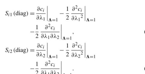
Another special case involves expanding the sensitivities in a Taylor series in theλmat3=1 (base case). If there are two sources and the Taylor series through first order inλmis integrated along the diagonal path, then (see Supplement)
Si1(diag)= ∂ci
∂λ1 3=
1
−1 2
∂2ci
∂λ12 3=
1
−1 2
∂2ci
∂λ1∂λ2
3=1
, (10)
Si2(diag)= ∂ci
∂λ2 3=1
−1 2
∂2ci
∂λ22 3=1
−1 2
∂2ci
∂λ1∂λ2 3=
1
. (11)
The cross term(−∂2ci/∂λ1∂λ2)is split evenly betweenSi1
andSi2. If the integration is done instead on the path B–b1–b
in Fig. 1, the full cross term is assigned toSi1and is absent
entirely fromSi2. Similarly, if the integration is along the
path B–b2–b, the full cross term is assigned toSi2and is
ab-sent fromSi1. Thus, the source contributions are the same for
these three paths except for the location of the cross term. Co-han et al. (2005) expandedciin a second-order Taylor series about3=1 and used it to develop source apportionments that are the same as Eqs. (10) and (11) except that they did not assign the cross term to the individual sources. The PIM shows that the cross term can be assigned to sources based on the emission-control path.
2.3 Analogy in thermodynamics
The dependence of the source contributions on path has an analogy in thermodynamics. For example, in the case of a single-component gas, the energy E is a function of the state variables: temperatureT, and volumeV. The change inE between two states of the system,1E, depends only on the initial and final values ofT andV. However, when
1Eis split into contributions from the heat exchange with the surroundings (RPdq) and the pressure (p)-related work (R
PpdV) in the equation,1E= R
Pdq− R
PpdV, the heat ex-change and work depend on the pathP from the initial to final states of the system. Thus, the concentrationsci from an air quality simulation may be regarded as analogous toE
and the emissions, initial and boundary concentrations, me-teorology and chemical mechanism as analogous toT andV. The1cibetween two simulations differing only in emissions can be allocated to sources, but this allocation is analogous to heat exchange and work and depends on the path along which the emissions are changed.
3 Model and inputs
20–22 June, beginning with clean initial concentrations in both cells. There was no transport into the cells via the lat-eral or top boundaries. The latitude was that of Los Angeles and Atlanta. The Carbon Bond 6 (CB6) chemical mechanism represented the gas-phase chemistry (Yarwood et al., 2012). The effect of the inputs is that cleaner air from the upper cell is entrained into the lower cell during the morning as the lower cell grows in height. Then, in the evening, the lower cell shrinks in height and leaves pollutants aloft in the upper cell. Consequently, there is carry-over of pollutants from day to day affecting the chemistry in the lower cell. Additional details of the simulations are in Table S1 (in the Supplement). The emissions were developed from the national totals in the 2008 US National Emission Inventory, version 3 (US EPA, 2013b) with several adjustments. Emissions from wildfires and prescribed fires were excluded because these vary greatly from year to year and were unusually high in 2008. Also, to represent summer conditions, emissions from residential wood combustion were excluded. Further, emis-sions of NO from lightning were added (Koo et al., 2010). The emissions were segregated into biogenic (plus lightning) emissions and five major source categories of anthropogenic emissions: fuel combustion, industrial sources, on-road ve-hicles, non-road veve-hicles, and other emissions. Vegetation and soil emissions and their speciation are from BEIS3.14 (Pierce et al., 1998). Anthropogenic emissions of volatile organic compounds (VOCs) from a major source category were allocated to CB6 species using speciation profiles from SPECIATE 4.3 for one or two sub-categories of sources comprising a significant fraction of the VOC emissions (Si-mon et al., 2010; US EPA, 2013a). The annual emissions of VOC species, NOx (=NO+NO2), CO, and HONO for
each source category were allocated to hours of a Wednes-day in June using temporal profiles (US EPA, 2013c). On a national scale, the biogenic VOC emissions are large com-pared to the anthropogenic VOC emissions, but this is not the case in urban areas. To represent better an urban area the anthropogenic emissions were weighted by a factor of 5 and the biogenic emissions by a factor of 1. A summary of the re-sulting daily emission rates for all source categories is given in Table 1, and the complete set of emission rates is in Ta-ble S2.
The model and inputs are not intended to be a detailed representation of a specific urban area but rather to provide a useful platform for testing the PIM, specifically different integration formulas and the dependence of the source con-tributions on paths.
4 Results
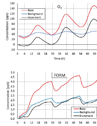
The concentrations of O3and formaldehyde (FORM) in the
background simulation (biogenic emissions only), the base simulation (both the biogenic and anthropogenic emissions) and the difference between the simulations (anthropogenic
Figure 2. Results from the two-cell model simulations. Ozone and formaldehyde concentrations for the base case and the background case and the difference between them (anthropogenic increment).
increment) are shown in Fig. 2. Similar plots for NO2 and
HNO3are in Fig. S1 in the Supplement. The peak O3
con-centration remains relatively constant over the 3 days in the background simulation (47–52 ppb) but increases steadily in the base simulation (from 75 ppb on day 1 to 151 ppb on day 3) due to the additional anthropogenic emissions on days 2 and 3 and the carryover of pollutants in the upper cell. Both O3 and FORM have sizeable concentrations in
the background case whereas NO2and HNO3have very low
concentrations due to the low biogenic NOx emissions. The O3 increment is negative at the beginning of day 1 due to
the titration of O3by the anthropogenic NO emissions. The
VOC/NOx ratio in the base case increases from 5–7 on day 1 to 9–20 ppbC ppb−1on day 3. Overall, the simulations provide a wide range of conditions for testing the PIM.
4.1 Accuracy of the numerical integration
The O3, FORM, NO2, and HNO3increments were allocated
to the five anthropogenic source categories and to the four species or groups of species emitted by each source cate-gory: VOC, CO, NOx, and HONO. Thus, a total of M= 20 sensitivities were calculated and integrated in the PIM. Source apportionments were determined for three emission-control paths: diagonal (Diag); VOC first (VOCF); and NOx first (NOxF). Along the Diag path, the scaling parameters
λVOCm =λCOm =λNOx
Table 1. Summary of daily emission rates used in the base-case simulation.
Emission rate (mol day−1km−2)
Biogenic Fuel Industrial On-road Non-road Other Species sourcesa combustion sources vehicles vehicles sources
NO 13.5 77.4 19.7 132.9 73.2 1.9
NO2 0.00 8.60 2.19 13.59 7.48 0.21 HONO 0.00 0.00 0.00 1.18 0.65 0.00 CO 35.9 51.8 58.2 1158.4 683.0 57.0 VOC 166.8 6.1 244.3 129.9 115.1 59.3 VOC/NObx 29.8 0.09 16.6 1.4 2.4 31.8
aIncludes lightning.bNO
x=NO+NO2. VOC/NOxunits are mole C (mole NOx)−1
treated equivalently. The VOCF path emphasizes initial con-trol of VOC and CO emissions followed by later concon-trol of NOxand HONO emissions, as defined byλVOCm =λCOm =u3 and λNOx
m =λHONOm =sin(π u/2), m=1, . . .,5. The NOxF path has the reverse assignments ofu3and sin(π u/2). View-ingλVOCm ,λCOm as analogous toλ1in Fig. 1 andλNOm x,λHONOm as analogous toλ2, then the VOCF path in 20-dimensional
space is analogous to Path 2 in Fig. 1 and the NOxF path is analogous to Path 3.
The Gauss–Legendre formula was tested for accuracy us-ing different numbers of integration points and different in-tegration variables. One set of tests, labeled GLns, used the distancesas the integration variable andnintegration points. Another set of tests, labeled GLnr, used a transformation of the variablestor=s1/2. Equation (4) then becomes
Sim(x, t;P )=
2
1 Z
0
∂ci(x, t;3)
∂λm 3=3
(s[r]) dλm
ds
s(r)
rdr. (12)
Because the background case contains no anthropogenic emissions, O3formation is strongly limited by the
availabil-ity of NOx. As a consequence, the sensitivity of O3 with
respect to any λm that scales NOx emissions is very large near3=0, but the sensitivity decreases very rapidly as NOx emissions are added. The transformation torhas two poten-tially beneficial effects for the source apportionment of O3.
First, the points for the numerical integration are chosen for the variabler. When transformed back to the variables, the points for s are closer to3=0 than ifs were the integra-tion variable, giving more resoluintegra-tion where the sensitivity is changing most rapidly. Second, the factor r in Eq. (12) re-duces the magnitude of the integrand nearr=s=λm=0, and makes the integrand identically 0 atr=0. This can yield an integrand that is easier to integrate. Finally, as a simple alternative, the source contributions were calculated by the trapezoidal rule using the two points at3=0 and 1 (labeled TR2).
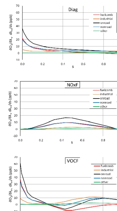
Figure 3. Dependence of the integrands for allocating O3to sources on the distancesalong the Diag, NOxF and VOCF paths. The inte-grand (Eq. 4) is calculated at the time of peak O3on day 3 (66 h).
gives the error and bias for NO2and HNO3. For comparison,
the mean absolute values of the increments1O3,1FORM, 1NO2, and1HNO3are 34.9, 1.52, 7.67, and 16.0 ppb,
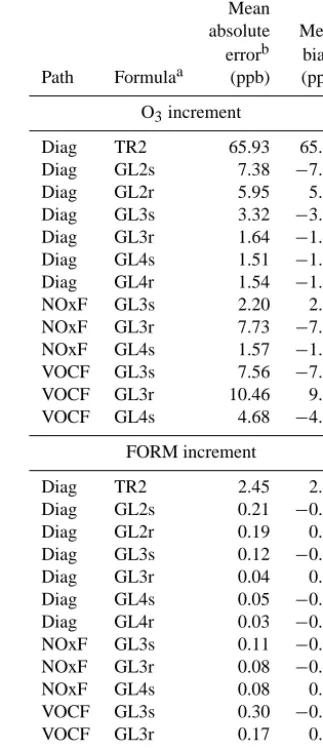
re-spectively. Though they use the same number of points, there is a large reduction in error and bias from TR2 to GL2s or GL2r, indicating the significant advantage of the GL formu-las. As the number of points included in the GLns or GLnr formulas increases, the error decreases for O3, FORM, and
NO2and generally the bias as well. There are some
excep-tions to this trend for HNO3, but these occur for cases where
the error and bias are already quite low (average error<4 % of the average increment). For O3 and the Diag path, the
GLnr formula gives more accurate results than the GLns for-mula for two or three points and essentially the same accu-racy for four points. For FORM, the GLnr formula is always more accurate than the GLns formula. The GLnr formula is usually less accurate than the GLns formula for NO2 and
HNO3and for O3with the NOxF and VOCF paths.
Table 2 also shows that the accuracy of a formula is lower for the VOCF path than the other paths when using the same number of points. This difference can be understood by ex-amining the integrand in Eq. (4). Figure 3 displays the inte-grands for allocating1O3to sources at the time of peak O3
on day 3, when it is most difficult to obtain good agreement between the sum of the source contributions and1O3. Along
the Diag and NOxF paths, the integrands have a constant cur-vature, either positive (Diag) or negative (NOxF), and the in-tegrands are mainly positive, with only small negative values nears=1. However, along the VOCF path, four of the in-tegrands have a positive curvature from s=0 tos=∼0.5, and then a negative curvature for the remainder of the path. Also, the integrands vary over a wider range along the VOCF path than the other paths. Further, the integrands for on-road vehicles and fuel combustion are both positive and negative, resulting in the cancellation of contributions to the integrals from different sections of the path. The change in curvature, wider range of variation and especially the cancellation of contributions require more points on the VOCF path to ob-tain an accurate integration.
Overall, the GL3r formula for the Diag path and the GL4s formula for the other paths give quite accurate results and were used to calculate the source apportionments in Sect. 4.2. Figure S2 gives a comparison of the sum of the source con-tributions vs. 1O3,1FORM, 1NO2, and1HNO3at each
hour of the simulation. The plots show again that the largest errors occur for the VOCF path.
4.2 Source apportionments
Figure 4 presents the apportionment of 1O3 to the five
source categories and four emission species using the Diag path. The VOC contributions are always positive, and the largest contributions are from industrial sources and on-road and non-road vehicles. The NOx contributions are small and primarily negative on day 1, when the atmospheric
Table 2. Average error and bias for different numerical integra-tion formulas. The sum of the source contribuintegra-tions calculated using the formula is compared to the anthropogenic increment of O3or FORM.
Mean
absolute Mean errorb biasb Path Formulaa (ppb) (ppb)
O3increment
Diag TR2 65.93 65.93 Diag GL2s 7.38 −7.36 Diag GL2r 5.95 5.71 Diag GL3s 3.32 −3.30 Diag GL3r 1.64 −1.49 Diag GL4s 1.51 −1.50 Diag GL4r 1.54 −1.49 NOxF GL3s 2.20 2.15 NOxF GL3r 7.73 −7.67 NOxF GL4s 1.57 −1.54 VOCF GL3s 7.56 −7.32 VOCF GL3r 10.46 9.62 VOCF GL4s 4.68 −4.63
FORM increment
Diag TR2 2.45 2.45 Diag GL2s 0.21 −0.20 Diag GL2r 0.19 0.19 Diag GL3s 0.12 −0.12 Diag GL3r 0.04 0.02 Diag GL4s 0.05 −0.04 Diag GL4r 0.03 −0.02 NOxF GL3s 0.11 −0.10 NOxF GL3r 0.08 −0.01 NOxF GL4s 0.08 0.08 VOCF GL3s 0.30 −0.30 VOCF GL3r 0.17 0.11 VOCF GL4s 0.09 −0.08
aTR2=trapezoidal rule, two points. GLnx= Gauss–Legendre formula usingnpoints andxas the integration variable.bHourly average over the 3-day simulation.
VOC/NOx<7.5 ppbC ppb−1in the base case. Under these conditions, NOxemissions tend to inhibit O3formation, and
hence the contributions are negative. On day 2, however, the NOx contributions become positive and then increase from day 2 to day 3. The total of the NOx contributions from all sources at 42 h is essentially the same as the total VOC con-tribution, and at 66 h, the total NOx contribution is twice the total VOC contribution. The increasing importance of the NOx contributions is due to the increasing VOC/NOx, which is 10–20 ppbC ppb−1 after 36 h, resulting in NOx -limited O3formation.
on-Figure 4. Contributions of sources and VOC, NOx, CO, and HONO emissions to the anthropogenic O3 increment. Results are for the Diag path.
road and non-road vehicles are not negligible compared to the VOC contributions of these sources. For on-road vehi-cles, the CO contributions are generally 20–45 % of the VOC contributions, and for non-road vehicles, 10–30 %. HONO emissions are assigned only to on-road and non-road vehi-cles and are small (0.8 % of NOx, Table 1). For both of these sources, their HONO emissions contribute<0.35 ppb to the
1O3.
Figure 5 displays the source contributions to 1O3
ob-tained with the three paths. (The contributions of all emission species from a source are combined together.) Results for the Diag and NOxF path are similar. For these paths, on-road vehicles have the largest and non-road vehicles the second-largest contributions during most of the simulation, and the “other” category contributes<3 ppb to 1O3. However,
in-dustrial sources are more important than fuel combustion for the Diag path, and the reverse is true for the NOxF path. The source contributions for the VOCF path are distinctly differ-ent. Over most of the simulation, the ranking of the contribu-tions is industrial sources>non-road vehicles>on-road ve-hicles, the opposite of the Diag path. Also, fuel combustion has a negative contribution over the entire simulation and the other category has a larger contribution (up to 6.5 ppb) than for the Diag and NOxF paths.
The different results for the VOCF path can be explained by the fact that the NOx emissions are controlled last on this path or, in terms of the integration, essentially only NOx emissions are added nears=0. The sensitivity of O3to these
emissions is large and positive nears=0 (Fig. 3) because the VOC/NOx ratio is high in the background case. However,
the VOC/NOx ratio decreases rapidly assincreases along the VOCF path, the sensitivity to NOx emissions becomes negative, and O3formation becomes VOC-limited for most
of the path. Thus, fuel combustion has a negative source con-tribution because its emissions are mostly NOx, and indus-trial sources have the largest positive contribution because they have the largest VOC emissions. Also, non-road vehi-cles have a larger contribution than on-road vehivehi-cles because both sources have a similar magnitude of VOC emissions but on-road vehicles have 82 % more NOxemissions, which sup-press O3formation on the VOC-limited section of the path.
The source contributions to1FORM for the three paths are also in Fig. 5. For the Diag path, the relative importance of the sources on days 2 and 3 is the same for1FORM as for 1O3, and this is also true for the NOxF path. For the
VOCF path, the on-road and non-road vehicles contribute more to 1FORM than the industrial sources, but the re-verse is true for the contributions of these sources to1O3.
The on-road and non-road vehicles have the largest contri-butions to1FORM on each path because these sources have the largest primary FORM emissions and the largest emis-sions of olefins, which are important precursors to secondary FORM from oxidation reactions (Table S2).
Figure S3 contains the apportionment of 1NO2 and 1HNO3 to sources. The source contributions to1NO2 for
the Diag and NOxF paths are quite similar; those for the VOCF path differ in that the contributions of the industrial sources and other category are primarily negative after 18 h. The source contributions to1HNO3for the Diag and NOxF
Figure 5. Apportionment of the anthropogenic O3increment (left) and the FORM increment (right) to sources using the Diag, NOxF, and VOCF emission-control paths.
in importance is the same as the ranking of their NOx emis-sions. The source contributions to 1HNO3 for the VOCF
path are similar to those for the other paths except that the contributions of non-road vehicles and fuel combustion are reversed in importance. The reversal is likely due to the much larger VOC emissions from non-road vehicles, which would enhance the oxidation of NOxon the VOC-limited part of the path.
5 Conclusions
As shown in Sect. 4, the PIM can allocate the difference in concentration between two simulations to emission sources. Consequently, the PIM requires that the base-case concen-tration minus the sum of the anthropogenic source contri-butions (difference δ)equals the background concentration (within the accuracy of the numerical integration). Other methods do not have this constraint. Ifδis less than the back-ground concentration, then the method assigns too much portance to the anthropogenic sources and will give the im-pression that reducing anthropogenic emissions will reduce the pollutant concentration more than will actually occur (over-allocation of the anthropogenic increment to the an-thropogenic sources). Similarly, ifδis greater than the
back-ground concentration, the method assigns too little impor-tance to the anthropogenic sources (under-allocation of the anthropogenic increment). The PIM ensures that the anthro-pogenic increments to O3 and the other species are neither
over- nor under-allocated to the anthropogenic sources. Another advantage is that the PIM is based on an exact mathematical relationship that is independent of the chem-istry or model and does not require added relationships or approximations. The PIM allows source contributions to be either positive or negative. If the secondary pollutant forma-tion is inhibited by emissions of some species, source, or ge-ographic area, the sensitivity to these emissions will be nega-tive for at least some values of the scaling parameterλm, and the integral in Eq. (2) may be negative.
Once a model has been modified to calculate the first-order sensitivities, the PIM requires only very simple post-processing of model results, specifically, calculating a linear combination of sensitivities from different simulations. This can be readily done with existing post-processing packages such as the Package for Visualization of Environmental data (PAVE) or the Visualization Environment for Rich Data In-terpretation (VERDI) (University of North Carolina, 2004, 2014). The PIM is not focused on just one species, e.g., O3.
generate all the information needed to allocate1cj for any other species j predicted by the model, and there is mini-mal additional effort needed to allocate 1cj for the second and subsequent species. Finally, the PIM highlights the im-portance of the background simulation. For a simulation with anthropogenic emissions included to be useful in designing emission controls, there is an implicit assumption that a sim-ulation without the anthropogenic emissions gives trations consistent with estimates for clean air. The concen-tration in the background simulation can be determined by an actual simulation or by subtracting the sum of all the source contributions from the base-case concentration.
In principle, there is an infinite number of source appor-tionments available from the PIM. However, each source ap-portionment is linked to an emission-control strategy. If a control strategy is defined along with the timing of the con-trols, the number of source apportionments is reduced to just one.
The major disadvantage of the PIM is that it requires more computational effort than other methods because the sensitiv-ities must be determined at several emission levels between the base and background simulations. This disadvantage is mitigated, to some degree, because the additional simulations provide information on how concentrations and sensitivities will change along the emission-control path.
The PIM has been applied in this work to a simplified con-figuration of CAMx that includes the nonlinear chemistry but not transport or dispersion. However, transport and disper-sion do not involve nonlinear interactions among the species. Because the nonlinear dependence of the sensitivities on the integration variable (Fig. 3) is driven by the nonlinear chem-istry and a full 3-D configuration should not have any other sources of nonlinearity, the number of integration points re-quired for PIM for a 3-D configuration should be similar to the number required for the simplified configuration (three or four) (Dunker et al., 2015).
Supplementary information
Application of the PIM to the special case involving the Tay-lor series expansion, input data and emissions for the model simulations, accuracy in allocating 1NO2 and 1HNO3 to
sources using different integration formulas, comparison of the sum of the source contributions to the anthropogenic in-crement at each hour, and source contributions to1NO2and 1HNO3.
The Supplement related to this article is available online at doi:10.5194/gmd-8-1763-2015-supplement.
Edited by: V. Grewe
References
Bowman, F. M.: A multi-parent assignment method for analyzing atmospheric chemistry mechanisms, Atmos. Environ., 39, 2519– 2533, 2005.
Bowman, F. M. and Seinfeld, J. H.: Ozone productivity of atmo-spheric organics, J. Geophys. Res., 99, 5309–5324, 1994. Butler, T. M., Lawrence, M. G., Taraborrelli, D., and Lelieveld, J.:
Multi-day ozone production potential of volatile organic com-pounds calculated with a tagging approach, Atmos. Environ., 45, 4082–4090, 2011.
Cohan, D. S., Hakami, A., Hu, Y., and Russell, A. G.: Nonlinear response of ozone to emissions: source apportionment and sensi-tivity analysis, Environ. Sci. Technol., 39, 6739–6748, 2005. Dunker, A. M.: Efficient calculation of sensitivity coefficients for
complex atmospheric models, Atmos. Environ., 15, 1155–1161, 1981.
Dunker, A. M.: The decoupled direct method for calculating sensi-tivity coefficients in chemical kinetics, J. Chem. Phys., 81, 2385– 2393, 1984.
Dunker, A. M., Yarwood, G., Ortmann, J. P., and Wilson, G. M.: The decoupled direct method for sensitivity analysis in a three-dimensional air quality model- implementation, accuracy, and ef-ficiency, Environ. Sci. Technol., 36, 2965–2976, 2002a. Dunker, A. M., Yarwood, G., Ortmann, J. P., and Wilson, G. M.:
Comparison of source apportionment and source sensitivity of ozone in a three-dimensional air quality model, Environ. Sci. Technol., 36, 2593–2964, 2002b.
Dunker, A. M., Koo, B., and Yarwood, G.: Source apportionment of the anthropogenic increment to ozone, formaldehyde, and nitro-gen dioxide by the path-integral method in a 3-D model, Envi-ron. Sci. Technol., 49, 6751–6759, doi:10.1021/acs.est.5b00467, 2015.
efunda: available at: http://www.efunda.com/math/num_ integration/findgausslegendre.cfm, last access: 29 January 2014.
Emmons, L. K., Hess, P. G., Lamarque, J.-F., and Pfister, G. G.: Tagged ozone mechanism for MOZART-4, CAM-chem and other chemical transport models, Geosci. Model Dev., 5, 1531– 1542, doi:10.5194/gmd-5-1531-2012, 2012.
ENVIRON: Comprehensive Air Quality Model with Extensions, available at: http://www.CAMx.com, last access: 15 May 2013. Grewe, V.: A generalized tagging method, Geosci. Model Dev., 6,
247-253, doi:10.5194/gmd-6-247-2013, 2013.
Grewe, V., Tsati, E., and Hoor, P.: On the attribution of contributions of atmospheric trace gases to emissions in atmospheric model applications, Geosci. Model Dev., 3, 487–499, doi:10.5194/gmd-3-487-2010, 2010.
Isaacson, E. and Keller, H. B.: Analysis of Numerical Methods, John Wiley, New York, 1966.
Kaplan, W.: Advanced Calculus, Addison-Wesley, Reading, Mas-sachusetts, 1959.
Koo, B., Dunker, A. M., and Yarwood, G.: Implementing the decou-pled direct method for sensitivity analysis in a particulate matter air quality model, Environ. Sci. Technol., 41, 2847–2854, 2007. Koo, B., Wilson, G. M., Morris, R. E., Dunker, A. M., and Yarwood,
Koo, B., Chien, C.-J., Tonnesen, G., Morris, R., Johnson, J., Sakulyanontvittaya, T., Piyachaturawat, P., and Yarwood, G.: Natural emissions for regional modeling of background ozone and particulate matter and impacts on emissions control strate-gies, Atmos. Environ., 44, 2372–2382, 2010.
Kwok, R. H. F., Napelenok, S. L., and Baker, K. R.: Implementa-tion and evaluaImplementa-tion of PM2.5 source contribuImplementa-tion analysis in a photochemical model, Atmos. Environ., 80, 398–407, 2013. Marmur, A., Park, S.-K., Mulholland, J. A., Tolbert, P. E., and
Rus-sell, A. G.: Source apportionment of PM2.5in the southeastern United States using receptor and emissions-based models: con-ceptual differences and implications for time-series health stud-ies, Atmos. Environ., 40, 2533–2551, 2006.
Mysliwiec, M. J. and Kleeman, M. J.: Source apportionment of sec-ondary airborne particulate matter in a polluted atmosphere, En-viron. Sci. Technol., 36, 5376–5384, 2002.
Napelenok, S. L., Cohan, D. S., Hu, Y., and Russell, A. G.: Decou-pled direct 3D sensitivity analysis for particulate matter (DDM-3D/PM), Atmos. Environ., 40, 6112–6121, 2006.
Pierce, T., Geron, C., Bender, L., Dennis, R., Tonnesen, G., and Guenther, A.: Influence of increased isoprene emissions on re-gional ozone modeling, J. Geophys. Res., 103, 25611–25629, 1998.
Simon, H., Beck, L., Bhave, P. V., Divita, F., Hsu, Y., Luecken, D., Mobley, J. D., Pouliot, G. A., Reff, A., Sarwar, G., and Strum, M.: The development and uses of EPA’s SPECIATE database, Atmospheric Pollution Research, 1, 196–206, 2010.
Stein, U. and Alpert, P.: Factor separation in numerical simulations, J. Atmos. Sci., 50, 2107–2115, 1993.
Tao, Z., Larson, S. M., Williams, A., Caughey, M., and Wuebbles, D. J.: Area, mobile, and point source contributions to ground level ozone: a summer simulation across the continental USA, Atmos. Environ., 39, 1869–1877, 2005.
Tong, D. Q. and Mauzerall, D. L.: Summertime state-level source-receptor relationships between nitrogen oxides emissions and surface ozone concentrations over the continental United States, Environ. Sci. Technol., 42, 7976–7984, 2008.
University of North Carolina: Package for Analysis and Visualiza-tion of Environmental Data, version 2.3, available at: http://www. ie.unc.edu/cempd/EDSS/pave_doc/EntirePaveManual.html (last access: 17 November 2014), 2004.
University of North Carolina: Visualization Environment for Rich Data Interpretation, version 1.5, available at: https://www. cmascenter.org/verdi/, last access: 17 November 2014.
US EPA: Carbon Bond and SAPRC Speciation Profiles, available at: http://www.cmascenter.org/download/data.cfm (last access: 19 November 2013), 2013a.
US EPA: 2008 National Emissions Inventory, Version 3, Tech-nical Support Document, September 2013-Draft, available at: http://www.epa.gov/ttn/chief/net/2008inventory.html (last ac-cess: 20 November 2013), 2013b.
US EPA: CAIR Platform Data, available at: http://www.epa. gov/ttn/chief/emch/temporal/index.html (last access: 24 Decem-ber 2013), 2013c.
Wagstrom, K. M., Pandis, S. N., Yarwood, G., Wilson, G. M., and Morris, R. E.: Development and application of a computa-tionally efficient particulate matter apportionment algorithm in a three-dimensional chemical transport model, Atmos. Environ., 42, 5650–5659, 2008.
Wang, H., Jacob, D. J., LeSager, P., Streets, D. G., Park, R. J., Gilliland, A. B., and van Donkelaar, A.: Surface ozone back-ground in the United States: Canadian and Mexican pollution influences, Atmos. Environ., 43, 1310–1319, 2009.
Wang, Z. S., Chien, C. J., and Tonnesen, G. S.: Development of a tagged species source apportionment algorithm to character-ize three-dimensional transport and transformation of precur-sors and secondary pollutants, J. Geophys. Res., 114, D21206, doi:10.1029/2008JD010846, 2009.
Yang, Y.-J., Wilkinson, J. G., and Russell, A. G.: Fast, direct sensi-tivity analysis of multidimensional photochemical models, Env-iron. Sci. Technol., 31, 2859–2868, 1997.
Yarwood, G., Morris, R. E., Yocke, M. A., Hogo, H., and Chico, T.: Development of a methodology for source apportionment of ozone concentration estimates from a photochemical grid model, in: Proceedings of the 89th Annual Meeting of the Air & Waste Management Association, Air and Waste Management Associa-tion, Pittsburgh, PA, Paper 96-TA23A.06, 1996.
Yarwood, G., Gookyoung, H., Carter, W. P. L., and Whitten, G. Z.: Environmental Chamber Experiments to Evaluate NOxSinks and Recycling in Atmospheric Chemical Mechanisms, Texas Air Quality Research Program Project 10-042, University of Texas, Austin, 2012.