R E S E A R C H
Open Access
Adding structure to land cover – using
fractional cover to study animal habitat use
Mirjana Bevanda
1*, Ned Horning
2, Bjoern Reineking
1,3, Marco Heurich
5, Martin Wegmann
4and Joerg Mueller
5Abstract
Background: Linking animal movements to landscape features is critical to identify factors that shape the spatial behaviour of animals. Habitat selection is led by behavioural decisions and is shaped by the environment, therefore the landscape is crucial for the analysis. Land cover classification based on ground survey and remote sensing data sets are an established approach to define landscapes for habitat selection analysis.
We investigate an approach for analysing habitat use using continuous land cover information and spatial metrics. This approach uses a continuous representation of the landscape using percentage cover of a chosen land cover type instead of discrete classes. This approach, fractional cover, captures spatial heterogeneity within classes and is therefore capable to provide a more distinct representation of the landscape. The variation in home range sizes is analysed using fractional cover and spatial metrics in conjunction with mixed effect models on red deer position data in the Bohemian Forest, compared over multiple spatio–temporal scales.
Results: We analysed forest fractional cover and a texture metric within each home range showing that variance of fractional cover values and texture explain much of variation in home range sizes. The results show a hump–shaped relationship, leading to smaller home ranges when forest fractional cover is very homogeneous or highly
heterogeneous, while intermediate stages lead to larger home ranges.
Conclusion: The application of continuous land cover information in conjunction with spatial metrics proved to be valuable for the explanation of home-range sizes of red deer.
Keywords: Fractional cover, Remote sensing, Land cover classification, Animal movement, Habitat selection, Mixed model
Background
Habitat use of animals is assumed to be mainly driven by forage availability and is a complex hierarchical pro-cess of behavioural responses and choices [1]. Individuals choose habitat that maximizes resources (e.g. food or shelter) and conditions necessary for survival and repro-duction [2], whereas these resources are influenced by temporal and spatial variations of the landscape [3]. Habi-tat selection is led by behavioural decisions and is shaped by the environment, leading to the observed habitat use [4].
*Correspondence: mirjana.bevanda@earth-observation.org
1Biogeographical Modelling, Bayreuth Center for Ecology and Environmental Research BayCEER, University of Bayreuth, Universitaetsstr. 30, 95447 Bayreuth, Germany
Full list of author information is available at the end of the article
A large majority of animals use certain areas without showing a territorial behaviour, referred to as home range. In contrast to territories, a home range has no defended borders [5]. Home ranges are generally defined as the spa-tial expression of all behaviours an animal performs in order to survive and reproduce [5]. Since home ranges link individual movement paths to dispersal and popula-tion dynamics, understanding why and how home range sizes vary between and among species is a fundamental issue in ecology. The current and prospective availability of large movement data sets and remotely sensed envi-ronmental information will allow further detailed analysis [6]. Progress in GPS–sensor receiver technology and satel-lite telemetry makes it possible to track animals over long time spans with high temporal and spatial resolution
and to analyse their habitat requirements and movement paths [7].
By studying variation in home range size and identifying the factors involved in such variation, we can identify how habitat influence individual’s habitat use [2] and therefore the variation in home ranges. A number of factors have been adressed for shaping variation in home range sizes, these include the environmental productivity and the het-erogeneity of the landscape [8-10]. Especially the availabil-ity of forage is a main driver shaping home range sizes [11]. A common trade–off often faced by many large mammals takes places when open habitats provide the best forage, while closed habitats provide shelter against predators and this may vary with different spatio–temporal scales [12].
Typically in habitat use studies the landscape is repre-sented with a categorical habitat map usually derived from a classification [13,14], while in other studies the land-scape is represented only by the dominant habitat type [15,16]. A variety of land cover classifications are routinely produced using remotely sensed data such as MODIS and AVHRR [17].
However, the way the landscape is defined is crucial for the analysis of habitat use. In many studies the landscape is defined in land cover categories, containing classes such as “meadows”, “forest” and “agriculture” [13,15] and it is common sense that different needs of an animal corre-sponds to different land cover types, for example “forest” as areas for shelter and therefore resting or hiding sites, and “meadows” as areas for forage sites [12].
However, landscapes rarely contain sharp borders between cover types although that is how they are por-trayed using a classical land cover classification approach. Moreover information about spatial variation within an a–priori defined land cover class is not provided when using a classification. A forest might vary spatially due to different age classes of the trees or small tree fall gaps which increase spatial heterogeneity. This within land cover variation is not captured by categorical maps.
Therefore we use a continuous land cover approach such as fractional cover for the inclusion of spatial varia-tion within classes for our analyses. Fracvaria-tional cover is a multiscale analysis combined with spatial prediction. This method is related to spectral unmixing methods [18]. The fractional cover image are typically created using a higher resolution land cover classification image to calculate frac-tional cover training data for lower resolution imagery. For each pixel of the coarse resolution image the percentage coverage for each land cover class within the high reso-lution is calculated and used for a spatial prediction of the land cover percentages. The percentage cover for the chosen land cover types per pixel of the coarse resolution image is provided as result.
With this approach a continuous land cover classifica-tion can be derived which captures the spatial structure
in a fine scale manner and this provides a more realistic and more ecologically meaningful representation of the landscape. Global maps with similar approaches of per-centage coverage already exist such as MODIS or AVHRR [19,20] however only at a coarse spatial resolution and not validated in the study area.
Furthermore in many habitat use studies forests have structural attributes like “dense forest” or “light forest” with corresponding functional effects, such as light for-est with plentiful food resources due to an for-established understory as enough sunlight can reach the forest floor. However, these structural attributes are often not vali-dated and instead they are implicitly assumed [21]. With the fractional cover approach these structural attributes can be addressed clearly.
In this study, we investigate the potential of continu-ous land cover information for habitat use of red deer in the Bohemian Forest. As habitat use leads to differing home range sizes, we investigate the potential of continu-ous land cover information and its spatial representation for the explanation of their variation in size. We hypoth-esize larger home ranges with increasing forest cover due to lower density of food resources. We test our hypothesis on different spatial (90%, 70% and 50% isopleths) and tem-poral scales (monthly, biweekly and weekly) to account for temporal and spatial differences.
Methods Study area
The study area is located in Central Europe in the Bohemian Forest, an area belonging to two national parks: the Bavarian Forest National Park on the German side of the border (240 km2) and the Šumava National Park on the Czech Republic side of the border (640 km2). These
protected areas are embedded within the Bavarian For-est Nature Park (3070 km2) and the Šumava Landscape
Protection Area (1000 km2). In its entirety, the area is
(Ips typographus). By 2007, this had resulted in the death of mature spruce stands over an area amounting to 5,600 ha [23,24].
Red deer data
From 2002–2011 red deer were caught during winter, using a procedure approved by the Government of Upper Bavaria, Germany. Red deer were captured and fitted with GPS collars (Vectronic Aerospace, Berlin, Germany) in box traps with side windows after they were lured in with food. Here no immobilization was necessary. A sec-ond approach was to tranquillize deer by dart gun where they were attracted by food [25]. We collared 80 deer (39 male, 41 female). Ten individuals were collared two or more times. As animals spend the winter in enclosures, we restricted the analysis temporally from May to the end of September. The most common protocol was to mark red deer in late winter and retrieve the collars after a year by collar drop–off or recapturing, allowing the collars to be used on new individuals. We removed spatial and tempo-ral false fixes (i.e. locations taken only a few seconds apart) beforehand. We defined the samples from the multiple collared animals over the single year as independent. As the schedule of the collars are adjusted to take a location every 15 min for one day of the week we took a random sample of animals with sequences of short time intervals to ensure that all locations have a minimum interval of one hour. The median accuracy of the GPS locations was 16.5 m [26].
Home range estimation
Home ranges were estimated with a commonly used approach, the fixed kernel method [27,28] using the ref-erence method for the smoothing factor h [29]. We used three different home range definitions to include a spa-tial scale and to investigate the effect on the core area (50% kernel) and a wider range (70% kernel, 90% kernel). In addition, all home range definitions were estimated on three temporal scales: monthly, biweekly and weekly. We only estimated home ranges for individuals with at least ten locations for a given temporal scale, after removing spatial and temporal outliers [30].
Representation of the landscape
For the calculation of fractional cover a high resolution classified image was derived from aerial images and was used for training. The classified image contained 26 cate-gories (different forest types such as coniferous, deciduous and mixed forest, and age classes such as mature, medium, young). Due to used spatial and spectral resolution we grouped those classes to three major categories in order to be able to discriminate them appropriately: forest (con-taining all forest types and age classes), open areas (e.g. meadows, regeneration areas, clear cut areas) and others
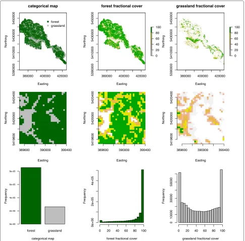
(e.g. water, rocks, roads). To create our training data the fractional cover of each class within 30 m Landsat pixels was calculated. The resulting percent cover values for a particular class were used as response variables to train a random forest (RF) regression model [31]. Random forest uses an ensemble of decision trees (in our case regression trees) to model non-linear relations among response vari-ables [32-34]. The resulting RF model was then used to predict percent cover for the cover type being modelled on a Landsat image using pixel spectral values as predic-tor variables. The number of regression trees used in the random forest model was 1000, the number of predictors tried on each split was set to the algorithm’s default value (number of Landsat image bands/3). An unbiased accu-racy assessment is provided by RF using “Out Of Bag” statistics calculated from a random selection of 1/3 of the training data [31]. Three cloud free Landsat 5 scenes (path 192, row 26) with bands 1–5 from 2006 (July 15th, October 19th) and 2009 (September 9th) were used for the fractional cover analysis. The three predicted vegetation layers complement each other and sum up to 100%. The class “others” contains only small values in our study area, therefore the major part of the values are split between “forest” and “grassland”. Since both layers complement each other we included only the class “forest” in our analysis. Figure 1 shows the categorical map and the frac-tional cover layers “forest” and “grassland” for the whole study area (upper panels). An enlarged display of a section shows how the formerly categorical representation of the landscape is now split up in continuous values (middle panels). The lower panels show the representation of the categorical values within the fractional cover values in a histogram. The discrete classes are represented by very high cover values within the study area (see Additional file 1: Figure S3 for a figure of the observed vs. predicted values of the regression model).
380000 400000 420000
5390000
5410000
5430000
5450000
categorical map
Easting
Northing
forest grassland
380000 400000 420000
5390000
5410000
5430000
5450000
forest fractional cover
Easting
Northing
0 20 40 60 80 100
380000 400000 420000
5390000
5410000
5430000
5450000
grassland fractional cover
Easting
Northing
0 20 40 60 80 100
Easting
Northing
389600 390000 390400
5419600
5420000
5420400
Easting
Northing
389600 390000 390400
5419600
5420000
5420400
Easting
Northing
389600 390000 390400
5419600
5420000
5420400
forest grassland
Frequency
0e+00 2e+05 4e+05 6e+05 8e+05
categorical map forest fractional cover
Frequency
0 20 40 60 80 100
0e+00
2e+05
4e+05
grassland fractional cover
Frequency
0 20 40 60 80 100
0
10000
30000
50000
Figure 1Overview of the landcover and fractional cover values within the study area.The upper panels show the distribution of the categorical (left hand side) and continuous fractional cover values (middel and right hand panel). The second row shows a zoom–in for better representation and the last row shows the distribution of the values for the whole study area.
pixel values within the home range. A moving window was used to calculate the texture metric for every pixel rela-tive to its direct neighbours (eight pixels around a centre pixel). We then averaged the resulting texture values to obtain one value for the home range to fit into the mixed model design. We chose to use the texture metric “con-trast”, as it shows the least size dependency (see Additional file 1: Figure S1 and is easy to interpret as a measure of local variation in the image and therefore an indicator of
landscape heterogeneity. Throughout the remaining text we will refer to the contrast metric as a texture metric or simply as texture.
not considered in the analysis. For simplicity we will refer to the standard deviation as variation of fractional cover values.
Furthermore we estimated the mean elevation of the home ranges using the 30 m ASTER Global Digital Ele-vation Map (GDEM) (http://asterweb.jpl.nasa.gov/gdem. asp).
The chosen variables showed no correlation with each other (Pearson’s correlation with the threshold set to 0.7, -0.7 respectively).
Statistical analysis
To investigate the influence of forest fractional cover and texture on home range sizes, we used linear mixed mod-els [37] on the log transformed home range areas (km2). Afterwards we ran a backfit on the t–values to derive the essential variables [38]. Preliminary analysis showed that the variables texture and elevation have a hump–shaped relationship with home range size in the red deer data and we therefore used a quadratic fit in the models.
Following the framework of Zuur et al. (2009) [39] for mixed effect models, we first identified the best structure for the random effect term. We fitted random intercepts for each individual (ID), different sexes and the year the locations were sampled, using the full model with respect to fixed effects terms and using the REML criterion for fitting. We started with the full random term and then simplified the model. Afterwards we compared the mod-els with an ANOVA and the best model was evaluated with the Akaike Information Criterion (AIC). For variable selection, models were fitted with a maximum likelihood criterion. We considered as fixed effects the mean value of the fractional cover layer forest within a home range, the standard deviation of fractional cover values within a home range, the texture metric contrast and elevation. The final models where fitted using the REML criterion. We derived minimal adequate models by backward step-wise selection using a t–value of 2 as a threshold for inclusion [38]. We repeated the analysis for the three defi-nitions of home range size and for the three defidefi-nitions of temporal scale.
We used the software tool R version 3.0.1 [40] for all analysis. The package “adehabitatHR” [28] was used for the kernel calculations, “raster” [41], “EBImage” [42] and “randomForest” [43] for creation of the environmental variables and “lmer” [37] and “LMERConvenienceFunc-tions” [38] were used for the statistical analyses.
Results
The fractional cover approach allows a differentiation of variations within land cover types, compared to cate-gorical classes. The spatial heterogeneity of within class variation is captured by this approach. The fit of the random forest regression model for the forest layer was
70.15%. The diversity of fractional cover values within the home range level can be seen in Figure 2. As outlined in Figure 1, the corresponding categorical values are rep-resented by the very high percentage values within the fractional Cover approach.
Home ranges of red deer show a high variation in size in our study area (Additional file 1: Table S1). We analysed the variation of home range sizes with a mixed model, using mean and standard deviation of the forest fractional cover, as well as the variable elevation and a texture metric. The main random effect in all models was the individual effect (variable ID) with an explained deviance of 0.26– 0.38% (Additional file 1: Table S3). The fixed effects of the most parsimonious models explained between 26.88% and 30.88% of the observed variation in home range size for red deer across the different spatio–temporal scales (Additional file 1: Table S2).
In all models the texture metric showed the high-est explained deviance (7.98%–14.72%) across scales and was the dominant variable explaining variation in home range size with a hump–shaped relationship (Figure S3, Additional file 1: Table S2). However, this hump–shaped relationship was only pronounced at the monthly time scale, whereas in the biweekly and weekly time scale this relationship changed to a negative linear relationship. The texture metric can be interpreted as an index for spatial heterogeneity in a given area. Hence, at larger temporal scales very homogeneous and very heterogeneous land-scapes are leading to small home ranges, while at smaller temporal scales only very heterogeneous landscapes lead to small home ranges.
Furthermore the variation of forest fractional cover (the standard variation) within a home range contributes sig-nificantly with an explained deviance of 7.22–11.59% and a positive relationship, leading to larger home ranges where the variation of forest fractional cover values is higher (Figure 3).
Additionally mean showed a positive effect (5.48– 7.12% explained deviance), with no effect on the monthly time scale kernel 50% isopleth (Additional file 1: Figure S2A).
Elevation had a hump–shaped effect on home range size and showed a low explanatory value of 0.35%–6.02% (Additional file 1: Figure S2B).
Discussion
381000 382000
5420500
5421500
categorical map
Easting
Northing
381000 382000
5420500
5421500
forest fractional cover
Easting
Northing
20 40 60 80 100
381000 382000
5420500
5421500
grassland fractional cover
Easting
Northing
20 40 60 80 100
forest grassland
Frequency
0 500 1000 1500 2000
categorical map forest fractional cover
Frequency
0 20 40 60 80 100
0
100
200
300
400
500
grassland fractional cover
Frequency
0 20 40 60 80 100
0
100
200
300
400
500
Figure 2Representation of the landscape for one home range with both approaches, the categorical and the continuous fractional cover.The lower panels show the distribution of the values within the home range for each approach.
continuous landscape data provide important information for modelling habitat use.
Red deer as a mixed feeder [44] has the ability to digest a broad spectrum of food items and benefits from forest edges and from the food supply of younger forest stands which show a low forest canopy cover and therefore have a pronounced understory, as sunlight can reach the ground. Mean forest fractional cover shows a positive relationship with home range size meaning that a higher proportion of dense forest will lead to larger home ranges. Whereas in forest patches with less crown cover and therefore more heterogeneous structure, food resources are more abun-dant which leads to smaller home ranges. This result is in support with other studies [14,45,46]. Mean forest frac-tional cover is a rather unsuitable derivative, as it averages all pixels within the home range. Nevertheless it shows a significant explanatory value and gives an overview of the overall forest structure within the home range.
The standard deviation of forest fractional cover val-ues captures the variability of valval-ues within a home range. High values indicate a wide spectrum of forest fractional cover and therefore a more heterogeneous landscape
while small values indicate a more homogeneous land-scape within the home range. Tufto et al. (1996) [11] have shown, that female roe deer adjust the size of their home range in response to food supply. In accordance to this study red deer home range sizes increase in our study area with increasing standard deviation and therefore with more heterogeneous forest fractional cover, leading to a higher amount of unfavourable forest habitat within the home range.
weekly
A
home range size [ log km
2 ]
monthly
90 %
spatial scale of home range kernel
standard deviation of forest fractional cover within home range [%]
−4
−2
0
2
4
0 10 20 30 40 50
−4
−2
0
2
4
0 10 20 30 40 50
50 %
B
weeklyhome range size [ log km
2 ]
monthly
90 %
spatial scale of home range kernel
texture measure contrast calculated within home range
−4
−2
0
2
4
0 0.2 0.4 0.6 0.8 1
−4
−2
0
2
4
0 0.2 0.4 0.6 0.8 1
50 %
Figure 3Plot of log–transformed home range sizes (km2) for red deer in relation to(A)the standard deviation of the forest fractional
[23]. These areas appear very homogeneous when calcu-lated with a texture metric but offer good habitat for deer, as different resources are provided in a small area, lead-ing to small home ranges, as both requirements, food and cover, are fulfilled at the same spot. Furthermore a hetero-geneous landscape, providing many different resources, leads to small home ranges as all the resources needed can be reached within a small distance. The hump–shaped effect flattens in the biweekly and weekly time scale and can only be described with a negative linear trend. How-ever, a pattern towards a hump–shaped distribution can be seen (Figure 3B). This result shows that the tempo-ral scale needs to be accounted for when analysing home ranges as they are likely to change not based on eco-logical patterns only but on the time scale of the study. The time period of the study is restricted to the summer months, therefore the resource cover can be regarded as static, i.e. not highly changing over the time, while the resource food is dynamic and depleting. Therefore food supply is the main force shaping home range size dur-ing summer. When large patches of dense forest occur within the home range, the texture value will increase. These areas provide shelter against predators, but provide only little food resources. Therefore, as food resources are regarded to be a main force shaping home range size, home ranges will increase in size with the inclusion of large patches of dense forest (intermediate values of tex-ture). Furthermore, these regeneration areas are located at higher altitude and are therefore explaining the effect of elevation, reflecting the importance of bark beetle areas in this study. Like the regeneration areas, elevation shows a hump–shaped fit leading to smaller home ranges where important resources are abundant [48].
It is known that other factors, like body mass, age, repro-ductive status or climatic parameters like temperature or rainfall have an effect on home range size (please see [46] for a more complete list) and it is likely, that by includ-ing these parameters, the explanatory value of the models could be increased. However, the best method to estimate home ranges is under debate. While we used at least 10 relocation points [30] to estimate our home ranges other studies suggest at least 20 relocation points [29].
The choice of environmental parameters is important for habitat use modelling. Using classified land cover requires clear definitions of the land cover types but def-initions often vary between different maps making them difficult to compare [49]. Moreover do these classes need to reflect the ecological requirements. An increased dis-crimination of different land cover types is often helpful to better describe a landscape but an increase in the number of land cover classes often results in lower per–class accu-racy. Using alternative information such as continuous cover can help to improve how a landscape is repre-sented in a model. Applying remote sensing time–series
data can be valuable to further discriminate land cover types and hence allow more fractional cover classes if dis-tinct temporal signature exist for the different targeted land cover types. Applying continuous land cover mation for environmental analysis provides detailed infor-mation about ecotones and within land cover variation. This research illustrates that fractional cover mapping has potential benefits for ecological research by avoiding cat-egorical values or sharp, most often artificial, boundaries in the landscape. However, the fractional cover approach requires more analytical steps including spatial prediction models and might therefore be potentially biased by the model used.
Conclusion
The study demonstrates that continuous land cover infor-mation can provide valuable inforinfor-mation about spa-tial within class variation as well as gradual vegetation changes, a feature that is not available when using discrete classes. This is especially relevant in movement ecol-ogy where a continuous representation of the landscape might be more ecological appropriate. However, to evalu-ate the added value of the fractional cover approach with regard to land cover classification or biophysical parame-ter further analysis are needed. Fractional cover mapping of different land cover types adds information, critical to ecological studies, beyond what traditional land cover categorical mapping can offer. As the synergy between remote sensing and ecology increases improved process-ing and analysis methods will continue to be developed which will have a positive impact on ecological research. These benefits will be especially important with the grow-ing interest in spatio–temporal movement pattern.
Additional file
Additional file 1: Additional file contains the: Overview of size dependency of the texture metrics; Overview of red deer home range sizes across spatio–temporal scales; Overview of fixed effects across spatio–temporal scales; Overview of random effect values; Plot of mean forest fractional cover values within home ranges across spatio–temporal scales; Plot of observed and predicted values of the forest fractional cover regression model.
Competing interests
The authors declare that they have no competing interests.
Authors’ contributions
MB performed the statistical analysis and was primarily responsible for writing the manuscript. MB, NH and MW drafted the manuscript and designed the species-environment interaction analysis. BR and JM contributed in the development of the animal movement and resource use approach and its statistical analysis. The movement data within the National Park Bavarian Forest was provided by JM and MH. All authors contributed to the writing of subsequent revisions and approved the final version.
Acknowledgements
3), and the Bavarian Forest National Park Administration. We kindly thank Ingo Brauer, Horst Burghart, Rüdiger Fischer, Martin Gahbauer, Helmut Penn, Michael Penn, and Lothar Ertl for technical support. We thank the anonymous reviewers for valuable comments which improved the manuscript
considerably.
Author details
1Biogeographical Modelling, Bayreuth Center for Ecology and Environmental
Research BayCEER, University of Bayreuth, Universitaetsstr. 30, 95447 Bayreuth, Germany.2American Museum for Natural History, Central Park West at 79th
Street, NY 10024-5192 New York, USA.3Unité de recherche écosystèmes
montagnards, Irstea, 2 rue de la Papeterie-BP 76, 38402 St-Martin-d’Hères, France.4Department of Remote Sensing, Remote Sensing for Biodiversity Unit,
University Wuerzburg, Oswald Kuelpe Weg 86, 97074 Wuerzburg, Germany.
5Bavarian Forest National Park, Department of Research and Documentation,
Freyunger Str. 2, 94481 Grafenau, Germany.
Received: 10 June 2014 Accepted: 11 December 2014
References
1. Gaillard J-M, Hebblewhite M, Loison A, Fuller M, Powell R, Basille M, Van Moorter B:Habitat-performance relationships: finding the right
metric at a given spatial scale.Philos Trans R Soc London, Ser B, Biol Sci
2010,365(1550):2255–2265.
2. Richard E, Said S, Hamann J-L, Gaillard J-M:Toward an identification of
resources influencing habitat use in a multi-specific context.PloS
one2011,6(12):29048.
3. Gustafson E:Quantifying landscape spatial pattern: what is the state
of the art?Ecosystems1998,1:143–156.
4. Johnson DH:The comparison of usage and availability
measurements for evaluating resource preference.Ecology1980,
61:65–71.
5. Burt W:Territoriality and home range concepts as applied to
mammals.J Mammalogy1943,24(3):346–352.
6. Wikelski M, Kays RW, Kasdin NJ, Thorup K, Smith Ja, Swenson GW:Going wild: what a global small-animal tracking system could do for
experimental biologists.J Exp Biol2007,210(Pt 2):181–186.
7. Tomkiewicz SM, Fuller MR, Kie JG, Bates KK:Global positioning system and associated technologies in animal behaviour and ecological
research.Philos Trans R Soc London, Ser B2010,365(1550):2163–2176.
8. Boyce M, Mao J, Merrill E, Fortin D:Scale and heterogeneity in habitat
selection by elk in Yellowstone National Park.Ecoscience2003,
10(4):421–431.
9. Nilsen E, Herfindal I, Linnell J:Can intra-specific variation in carnivore home-range size be explained using remote-sensing estimates of
environmental productivity?Ecoscience2005,12(1):68–75.
10. Saïd S, Gaillard J-M, Widmer O, Débias F, Bourgoin G, Delorme D, Roux C: What shapes intra-specific variation in home range size? A case
study of female roe deer.Oikos2009,118(9):1299–1306.
11. Tufto J, Andersen R, Linnell J:Habitat use and ecological correlates of
home range size in a small cervid: the roe deer.J Animal Ecol1996,
65(6):715–724.
12. Godvik IMR, Loe LE, Vik JO, Veiberg VO, Langvatn R, Mysterud A: Temporal scales, trade-offs, and functional responses in red deer
habitat selection.Ecology2009,90(3):699–710.
13. Torres RT, Virgós E, Santos Ja, Linnell JDC, Fonseca C:Habitat use by
sympatric red and roe deer in a Mediterranean ecosystem.Animal
Biol2012,62(3):351–366.
14. Massé A, Côté SD:Linking habitat heterogeneity to space use by large herbivores at multiple scales: From habitat mosaics to forest
canopy openings.Forest Ecol Manage2012,285:67–76.
15. Börger L, Franconi N, Ferretti F, Meschi F, De Michele G, Gantz A, Coulson
T:An integrated approach to identify spatiotemporal and
individual-level determinants of animal home range size.Am
Naturalist2006,168(4):471–485.
16. Rivrud IM, Loe LE, Mysterud A:How does local weather predict red
deer home range size at different temporal scales?J Animal Ecol2010,
79(6):1280–1295.
17. Friedl MA, McIver DK, Hodges JCF, Zhang XY, Muchoney D, Strahler AH, Woodcock CE, Gopal S, Schneider A, Cooper A, Baccini A, Gao F, Schaaf C:
Global land cover mapping from MODIS: algorithms and early
results.Remote Sensing Environ2002,83(1-2):287–302.
18. Asner GP, Heidebrecht KB:Spectral unmixing of vegetation, soil and dry carbon cover in arid regions: Comparing mulitspectral and
hyperspectral observations.Int J Remote Sensing2002,
23(19):3939–3958.
19. DeFries R, Hansen M, Townshend JRG, Janetos AC, Loveland TR:A new global 1 km data set of percent tree cover derived from remote
sensing.Global Change Biol2000,6:247–254.
20. DiMiceli CM, Carroll ML, Sohlberg RA, Huang C, Hansen MC, Townshend JRG:Annual Global Automated MODIS Vegetation Continuous Fields (MOD44B) at 250 M Spatial Resolution for Data Years Beginning Day 65, 2000 -2010, Collection 5 Percent Tree Cover. College Park, MD, USA: University of Maryland; 2011.
21. Debeljak M, Dzeroski S, Jerine K, Kobler A, Adamic M:Habitat suitability modelling for red deer (Cer6us elaphus L.) in South-central Slovenia
with classification trees.Ecol Modell2001,138:321–330.
22. Fischer HS, Winter S, Lohberger E, Jehl H, Fischer A:Improving transboundary maps of potential natural vegetation using
statistical modeling based on environmental predictors.Folia
Geobotanica2013,48(2):115–135.
23. Müller J, Bußler H, Goßner M, Rettelbach T, Duelli P:The European spruce bark beetle Ips typographus in a national park: from pest to
keystone species.Biodivers Conserv2008,17(12):2979–3001.
24. Lausch A, Heurich M, Fahse L:Spatio-temporal infestation patterns of Ips typographus (L.) in the Bavarian Forest National Park, Germany.
Ecol Indicators2013,31:73–81.
25. Heurich M:Berücksichtigung von Tierschutzaspekten beim Fang und
der Markierung von Wildtieren.InInternationale Fachtagung zu Fragen
Von Verhaltenskunde, Tierhaltung und Tierschutz. 2011, 142–158. 26. Stache A, Löttker P, Heurich M:Red deer telemetry: dependency of the
position acquisition rate and accuracy of GPS collars on the
structure of a temperate forest dominated by European beech.Silva
Gabreta2012,18(1):35–48.
27. Worton B:Kernel methods for estimating the utilization distribution
in home-range studies.Ecology1989,70:164–168.
28. Calenge C:The package “adehabitat” for the R software: a tool for
the analysis of space and habitat use by animals.Ecol Modell2006,
197(3-4):516–519.
29. Kernohan BJ, Gitzen RA, Millspaugh JJ:Analysis of animal space use
and movements.InRadio Tracking and Animal Populations. Edited by
Millspaugh JJ, Marzluff J. San Diego, California, USA: Academic Press; 2001:126–164.
30. Börger L, Franconi N, De Michele G, Gantz A, Meschi F, Manica A, Lovari S, Coulson T:Effects of sampling regime on the mean and
variance of home range size estimates.J Animal Ecol2006,
75(6):1393–1405.
31. Breiman L:Random forests.Machine Learning2001,45(1):5–32. 32. Hansen MC, DeFries RS, Townshend JRG, Sohlberg R, Dimiceli C, Carroll M:
Towards an operational MODIS continuous field of percent tree
cover algorithm: examples using AVHRR and MODIS data.Remote
Sensing Environ2002,83(1-2):303–319.
33. Hansen MC, DeFries RS, Townshend JRG, Carroll M, Dimiceli C, Sohlberg
Ra:Global percent tree cover at a spatial resolution of 500 meters:
first results of the MODIS vegetation continuous fields algorithm.
Earth Interact2003,7(10):1–15.
34. Hayes DJ, Cohen WB, Sader Sa, Irwin DE:Estimating proportional change in forest cover as a continuous variable from multi-year
MODIS data.Remote Sensing Env2008,112(3):735–749.
35. Haralick R, Shanmugam K, Dinstein I:Textural features for image
classification.IEEE Trans Syst Man Cybernetics1973,3(6):610–621.
36. Dormann CF, Elith J, Bacher S, Buchmann C, Carl G, Carré G, Marquéz JRG, Gruber B, Lafourcade B, Leitao PJ, Münkemüller T, McClean C, Osborne PE, Reineking B, Schröder B, Skidmore AK, Zurell D, Lautenbach S:
Collinearity: a review of methods to deal with it and a simulation
study evaluating their performance.Ecography2013,36:27–46.
37. Bates D, Maechler M, Bolker B:lme4: Linear mixed-effects models
using S4 classes.R package version 0.92011.
38. Tremblay A, Ransijn J:LMERConvenienceFunctions: A suite of functions to back-fit fixed effects and forward-fit random effects, as
39. Zuur AF, Ieno EN, Walker NJ, Saveliev AA, Smith GM:Mixed Effects Models and Extensions in Ecology with R: Springer; 2009:596.
40. Development Core Team R:R: A Language and Environment for Statistical Computing: R Foundation for Statistical Computing; 2013.
41. Hijmans RJ:raster: Geographic data analysis and modeling; 2013. 42. Pau G, Oles A, Smith M, Sklyar O, Huber W:EBImage - Image processing
toolbox for R.R package version 4.2.12013.
43. Liaw A, Wiener M:Classification and regression by random forest.
R News2002,2(3):18–22.
44. Albon SD, Langvatn R:Plant phenology and the benefits of migration
in a temperate ungulate.Oikos1992,65:502–513.
45. Owen-Smith N, Fryxell JM, Merrill EH:Foraging theory upscaled: the
behavioural ecology of herbivore movement.Philos Trans R Soc
London, Ser B, Biol Sci2010,365(1550):2267–2278.
46. van Beest FM, Rivrud IM, Loe LE, Milner JM, Mysterud A:What determines variation in home range size across spatiotemporal scales in a large
browsing herbivore?J Animal Ecol2011,80(4):771–785.
47. Bevanda M, Fronhofer EA, Heurich M, Müller J, Reineking B:Landscape configuration is a major determinant of home range size variation; 2014. in prep.
48. Anderson LO, Shimabukuro YE, Arai E:Cover: Multitemporal fraction images derived from Terra MODIS data for analysing land cover
change over the Amazon region.Int J Remote Sensing2005,
26(11):2251–2257.
49. Herold M, Mayaux P, Woodcock CE, Baccini A, Schmullius C:Some challenges in global land cover mapping: An assessment of
agreement and accuracy in existing 1 km datasets.Remote Sensing
Env2008,112(5):2538–2556.
Submit your next manuscript to BioMed Central and take full advantage of:
• Convenient online submission
• Thorough peer review
• No space constraints or color figure charges
• Immediate publication on acceptance
• Inclusion in PubMed, CAS, Scopus and Google Scholar
• Research which is freely available for redistribution