A Note on the Asymmetry and Persistency of Shocks
in Malaysian Exchange Rate Volatility
Fardous Alom
Ministry of Civil Aviation and Tourism, Bangladesh
Abstract:This study attempts to examine the asymmetry and persistency of exchange rate volatility of the Malaysian ringgit against the USD, British pound, EURO, Japanese yen, and Singapore dollar within the framework of asymmetric component GARCH models using daily data over the period of 1st August 2005 to 24th April 2014. The empirical
findings reveal mixed evidence vis-à-vis asymmetry and persistency of exchange rate shocks to the volatility of Malaysian currency against different currencies considered in the study. The estimated results exhibit that the volatility of Malaysia’s exchange rate returns can be modelled with GARCH-type conditional variance models which capture volatility characteristics well. The volatility shocks to the Malaysia’s exchange rate are found to be highly persistent against the USD while reasonably persistent against the EURO, British pound, Japanese yen and Singapore dollar. Asymmetric effects of shocks to the volatility of Malaysia’s exchange rate against the USD, EURO and the Japanese yen are evident implying positive and negative shocks pose different effects to the volatility while symmetric effects of shocks to volatility are recorded for the British Pound and Singapore dollar. The empirical findings of this study provide insights to policymakers and practitioners.
Keywords: Asymmetry, exchange rate, Malaysia, persistency, volatility JEL classification: C58, F30, F31
1. Introduction
Following the collapse of the Bretton Woods agreement of the fixed exchange rate system in the early 1970s, world economies have started moving to the free-floating exchange rates allowing fluctuation of their currencies based on the market forces of demand and supply. However, the fluctuations or volatilities of exchange rates posture the economies in a state of unknown risk. Thus, a clear understanding of exchange rate volatility is essential due to its involvement with uncertainty and adjustment costs, structure of output, firm size, international investment, price fluctuation, competition and concentration of output as well as macroeconomic policy issues (Carter, 1984).
Given the importance of comprehension of exchange rate volatility, noteworthy efforts have been put forward by academic as well as institution level researchers. Exchange rate volatility has been explained from the viewpoints of macroeconomic fundamentals such as interest rates, inflation, trade accounts and debt by many researchers (Almeida, Goodhart, & Payne, 1998; Andersen, Bollerslev, Diebold, & Vega, 2002; Engel & West,
2005; Kim, McKenzie, & Faff, 2004; Laakkonen & Pankki, 2004; Meese & Rogoff, 1983). Modelling volatility characteristics of the exchange rate has emerged in three dimensions such as intraday periodicity, autocorrelation and discontinuities in prices
(Erdemlioglu, Laurent, & Neely, 2012). Autocorrelation modelling or modelling the conditional variance was done during the 1980s and took into consideration the stylised facts of volatility such as volatility clustering and persistence, leptokurtosis, leverage or threshold effects, and long memory in the fashion of financial assets. Diebold and Nerlove (1989), using multivariate latent factor autoregressive conditional heteroskedasticity (ARCH) model, provide evidence that ARCH models capture exchange rate volatility well. Hsieh (1989), using generalised ARCH (GARCH) and exponential GARCH (EGARCH) model, showed that volatility in the Canadian exchange rate data is captured quite well while Swiss and Dutch exchange rate volatility are captured reasonably well. Baillie and Bollerslev (1989) note that the conditional variance model or GARCH model captures daily, weekly or monthly volatility characteristics of exchange rate data. Bollerslev (1990) also modelled the movement of short-run nominal exchange rates within the framework of multivariate GARCH and reported that the multivariate GARCH model adequately captures co-movement of currencies.
Initial efforts on the ability of capturing volatility by GARCH-type models were followed by the development and application of GARCH models to identify symmetric effects. What this means is that positive and negative shocks exert the same effects on volatility and asymmetric effects implying the impacts of a negative shock are not fully compensated by the positive shock or that negative and positive shocks have different impacts on volatility along with short-run and long-run persistence of shocks to volatility. Evidence of volatility persistence and/or asymmetry in exchange rate is provided in many studies (Abdalla, 2012; Insah, 2013; Karuthedath & Shanmugasundaram, 2012; Maana, Mwita, & Odhiambo, 2010; McKenzie & Mitchell, 2002; Miron & Tudor, 2010; Narayan, Narayan, & Prasad, 2008; Yasir, Usman, & Muhammad, 2012; Yoon & Lee, 2008).
Most of the studies mentioned above were conducted in the context of developed countries and other parts of the developing world. To the best of our current knowledge, there is only one study covering the Malaysian exchange rate data. It is to be noted that Malaysia is also exposed to exchange rate volatility risk as in the case of other countries. During the 1997-98 financial crises, the exchange rate of the Malaysian ringgit against USD fell by over 37% between 1st July 1997 and 8th September 1998 compelling the country to
peg the ringgit against the USD at a rate of 3.8 ringgit per USD and this rate was maintained for about eight years (Hasan, 2002). The only study conducted in the context of Malaysia is that of Tse & Tsui (1997) that used data from 1978 to 1994 within the framework of the asymmetric Power ARCH (APARCH) model. They found that the APARCH model captures movements of currency quite well and asymmetric effects exist showing negative shocks reduce volatility more than the positive shocks. The dearth of studies in the Malaysian context provides the premise for a further understanding of the volatility pattern of the Malaysian exchange rate against selected major currencies such as the USD, British pound (GBP), EURO, Japanese yen (JPY, in hundreds) and the Singapore dollar (SGD).
There is a justification for these currencies to be selected. First, the Malaysian ringgit (RM) was pegged to the GBP until the collapse of the Bretton Woods system and from
17th June 1972 Malaysia switched from GBP to USD. Hence, the Malaysian currency has a
the exchange rate value is fixed. SGD is selected because this currency is heavily used for trading with Malaysia given that Singapore is a neighbour country. Apart from the above reasons, it should also be noted that Malaysia has high trade intensity with these countries.
The present study is distinct from other studies in three aspects. First, our study uses recent daily exchange rate data covering the period from August 2005 to April 2014 while previous studies used data up to 1994 only. Second, we employ the sophisticated asymmetric component generalised autoregressive conditional heteroskedasticity (ACGARCH) model to capture permanent and transitory volatility persistence along with asymmetric effects of shocks to the volatility, if any exist, which has been previously used by only a few studies. Identifying asymmetry is crucial because asymmetry implies that policy responses should be different. Of particular interest is the fact that over the study period, the cumulative sum of positive changes and the cumulative sum of negative changes of Malaysian exchange rates are not of the same magnitude. Third, we estimate models to assess asymmetry and persistency of RM’s volatility not only against the USD but also against the GBP, EURO, JPY and SGD with the expectation that volatility characteristics will differ from one numeraire to another. This is because these selected countries have different economic characteristics in terms of trade dominance in the world market, GDP, balance of trade and policies.
The rest of the paper is organised as follows. The next section addresses the source and nature of data while Section 3 explains the methodology used to estimate and analyse data. Section 4 reports the empirical findings and discusses the results while the last section concludes the paper.
2. Data and Their Properties
The study utilises daily data of the Malaysian exchange rate against the USD, GBP, EURO, JPY and SGD over the period 1st August 2005 to 24th April 2014, resulting in a total of 2155
observations. Initially, the plan was to work with data just after the financial crisis of 1997 but all series were not available because the Malaysian ringgit was pegged to the USD
from 2nd September 1998 to 21st July 2005. We therefore chose the start date to be from 1st August 2005. Data from the central bank of Malaysia, Bank Negara Malaysia, was used.
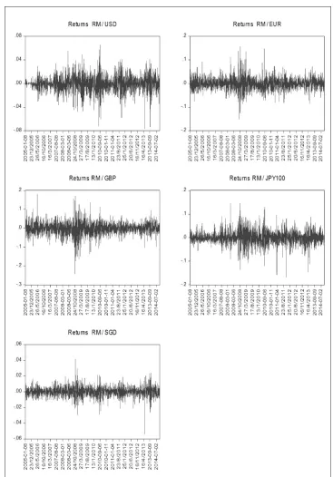
Returns of exchange rates are computed by using standard continuously computed logarithm technique as shown in equation (1) where Et is the exchange rate of current day
and Et-1 represents exchange rate of previous day:
(1)
that the distribution of the series is relatively peaked rather than normal. ADF statistics at the level and at first difference demonstrate that all series are non-stationary. Jarque-Bera test statistics also indicate that the series are non-normal. Figure 2 demonstrates considerable volatility clustering, meaning a rise in volatility is followed by another large rise and vice versa.
3. Modelling Framework
To model financial characteristics of time series data, Engle (1982) developed the ARCH model which was later generalised by Bollerslev (1986) as GARCH models. Following this, ARCH/GARCH models started to grow in different dimensions not only for magnitudes but also on the directions to better capture the financial characteristics of assets (Engle, 2001). One of these extended versions of GARCH-type models is the Component GARCH (CGARCH) model developed by Engle and Lee (1993). In the current study, we use the CGARCH model due to its superior performance over different aspects. As stated by Black and McMillan (2004), the CGARCH model decomposes conditional variances into a long-run time-varying trend component and a short-long-run transitory component, which reverts to the trend following a shock. This model has superiority in terms of capturing both long and short-run properties of time series. Christoffersen, Jacobs, Ornthanalai, and Wang (2008) state, “The component model’s superior performance is partly due to its improved
Rates RM/USD RM/GBP RM/EURO RM/JPY RM/SGD
Mean 3.3330 5.6760 4.4814 3.442 2.3939
Median 3.2835 5.3970 4.5168 3.3931 2.3959
Maximum 3.7825 7.1358 5.1859 4.1890 2.6332
Minimum 2.9385 4.5633 3.8158 2.7771 2.2152
Std. Dev. 0.2359 0.8243 0.3471 0.3632 0.0953
Skewness 0.3313 0.3980 -0.0141 0.0708 0.2805
Kurtosis 1.8727 1.5076 1.9439 1.7154 2.3521
JB 153.966 257.598 100.486 150.389 66.142
(prob.) (0.000) (0.000) (0.000) (0.000) (0.000)
ADF -1.9798 -1.2135 -1.7184 -1.7381 -0.9532
(prob.) (0.295) (0.670) (0.421) (0.411) (0.771)
Returns
Mean -0.0068 -0.0088 -0.0009 -0.0030 0.0061
Median 0.0000 -0.0029 -0.0107 -0.0254 0.0087
Maximum 1.9832 2.9377 3.5888 4.4778 1.7346
Minimum -2.5616 -4.0767 -3.0769 -4.5034 -2.2140
Std. Dev. 0.4005 0.5881 0.5635 0.8057 0.2507
Skewness -0.2038 -0.3301 0.2535 0.0541 -0.2315
Kurtosis 6.2063 7.2422 6.5182 6.1487 8.3146
JB 940.244 1658.931 1137.186 893.360 2561.407
(prob.) (0.000) (0.000) (0.000) (0.000) (0.000)
ADF -46.232 -33.822 -44.167 -48.581 -46.154
(prob.) (0.000) (0.000) (0.000) (0.000) (0.000)
Observations 2154 2154 2154 2154 2154
ability to model the smirk and the path of spot volatility, but its most distinctive feature is its ability to model the volatility term structure.”
In order to estimate the exchange rate volatility characteristics of Malaysia along with asymmetry assessment, CGARCH (1, 1) models in asymmetric form termed as ACGARCH (1, 1) is used. Towards this end, the ARMA–ACGARCH-M (1,1) model can be written in the following general form:
Mean equation:
(2)
Variance equations:
(3)
where REt refers to returns of exchange rate, β2 and β3 measure autoregressive and moving average coefficients, qt is the permanent component, (
e
t2−1−
h
t−1) serves as the drivingforce for the time-dependent movement of the permanent component and (
h
t−1−
q
t−1)represents the transitory component of the conditional variance. The sum of parameters
γ4 and γ6 measure the transitory shock persistence and γ2 measures long-run or permanent persistence derived from the shock to a permanent component given by γ3, while γ5
provides a measure of the asymmetry of the shocks to the volatility. k measures the
time lag where the lag order of ARMA is set by the methodology of Box-Jenkins (1976), hence the lag orders selected may differ across the series depending on the nature of the particular data. Models are selected based on the lowest AIC, highest R-squared and maximum likelihood values. Considering possible violation of normality, as noted earlier, models are estimated using generalised error distribution (GED).
4. Empirical Results
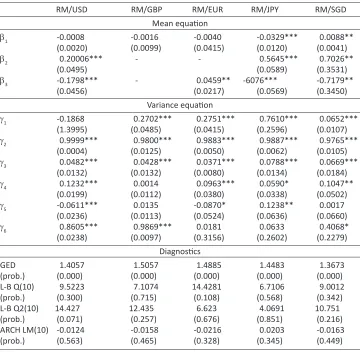
Table 2 presents estimates of the ARMA-ACGARCH model. With regard to RM/USD, ARMA (1, 1)-ACGARCH (1, 1) is estimated. Except for the constant term, the AR and MA terms are statistically significant at 1% level under mean equation implying that RM/USD return is influenced both by its own lag and residual lags. All the parameters in variance equation are statistically significant at 1% level with appropriate signs. Statistical significance of all parameters suggests that lagged residuals and lagged conditional variance are capable of explaining the conditional volatility and also that the shocks have both transitory and permanent effects on the volatility. The measure for long-run persistence parameter, γ2,
parameters of a GARCH(1, 1) model. In our CGARCH model, the calculation is performed by the following procedure. As γ2 measures long-run persistency, the half-life for long-run persistence is calculated as L . Since γ4 and γ6 measure transitory persistency, the half-life for transitory persistence is calculated as H.L .
The half-life of decay for RM/USD is 6932 days meaning the effects of shocks to the volatility in the long-run stays permanently or dies out extremely slowly. The half-life of decay for short-run persistence is 43 days or a slightly higher than a month.The sum
of transitory persistence parameters (γ4 and γ6) is less than the long-run persistence parameters; implying a slower mean reversion in the long-run. The asymmetry parameter,
γ5, is statistically significant at 1% level with a negative sign. The negative sign of γ5 implies that the negative shocks have a higher impact on the next period’s conditional volatility of exchange rate than positive shocks or in other words, depreciation shocks of RM against USD have a higher impact on the conditional volatility than appreciation shocks. This result is consistent with that of Tse and Tsui (1997).
For RM/GBP returns, ARMA (0, 0)-ACGARCH (1, 1) model suits well as suggested by the Box-Jenkins method. In this case, almost all parameters are statistically significant except for one of the transitory persistence parameter γ4 and asymmetry parameter γ5 implying the absence of asymmetric effects of shocks to the volatility or in other words, both positive and negative shocks have the same effects on the volatility of RM/GBP exchange rate returns. The long-run persistence parameter γ2 suggests moderate persistency of shocks to the volatility. The average half-life of decay of the effects of shock is 35 days. The half-life of transitory persistence is 58 days which is higher than long run persistence and which is also transitory in this case. The sum of transitory parameters, (γ4 and γ6), is
higher than the permanent persistence parameter indicating speedy mean reversion in the long-run or in other words the effects of shocks to the volatility die out very rapidly.
ARMA (0, 1)-ACGARCH (1, 1) model captures data well for RM/EURO exchange rate returns. All the parameters in variance equation are statistically significant except for γ6. The long-run persistence parameter signals relatively high persistence of shocks on the volatility. The average half-life of a shock to decay is around 60 days. The half-life in the short-run is just 1 day or almost no persistence. The sum of transitory parameters is lower than the permanent parameter, implying slower mean reversion in the long-run. The estimates also show that the asymmetry parameter γ5 is statistically significant and that it has a negative sign indicating that the negative shocks have higher impacts on the next period’s conditional volatility than the positive shocks.
The lower panel of Table 2 shows the results of diagnostic validity. It can be seen that the GED parameters for all models are less than 2 and are statistically significant at 1 % level of significance suggesting the possible violation of normality and appropriateness of using generalised error distribution instead of normal. No form of serious misspecification is detected as the Ljung-Box statistics at the level and squared along with ARCH-LM are not statistically significant at any level.
To sum up, the above discussion highlights that the RM/USD volatility maintains the same pattern for a long period as found in Tse and Tsui (1997), even after passing through the financial crises of 1997-98. Our study consistently reconfirms that any shock to RM/ USD maintains persistent and asymmetric effects on the volatility. The high persistence
RM/USD RM/GBP RM/EUR RM/JPY RM/SGD
Mean equation
β1 -0.0008 -0.0016 -0.0040 -0.0329*** 0.0088**
(0.0020) (0.0099) (0.0415) (0.0120) (0.0041)
β2 0.20006*** - - 0.5645*** 0.7026**
(0.0495) (0.0589) (0.3531)
β3 -0.1798*** - 0.0459** -6076*** -0.7179**
(0.0456) (0.0217) (0.0569) (0.3450)
Variance equation
γ1 -0.1868 0.2702*** 0.2751*** 0.7610*** 0.0652***
(1.3995) (0.0485) (0.0415) (0.2596) (0.0107)
γ2 0.9999*** 0.9800*** 0.9883*** 0.9887*** 0.9765*** (0.0004) (0.0125) (0.0050) (0.0062) (0.0105)
γ3 0.0482*** 0.0428*** 0.0371*** 0.0788*** 0.0669*** (0.0132) (0.0132) (0.0080) (0.0134) (0.0184)
γ4 0.1232*** 0.0014 0.0963*** 0.0590* 0.1047**
(0.0199) (0.0112) (0.0380) (0.0338) (0.0502)
γ5 -0.0611*** 0.0135 -0.0870* 0.1238** 0.0017
(0.0236) (0.0113) (0.0524) (0.0636) (0.0660)
γ6 0.8605*** 0.9869*** 0.0181 0.0633 0.4068*
(0.0238) (0.0097) (0.3156) (0.2602) (0.2279) Diagnostics
GED 1.4057 1.5057 1.4885 1.4483 1.3673
(prob.) (0.000) (0.000) (0.000) (0.000) (0.000)
L-B Q(10) 9.5223 7.1074 14.4281 6.7106 9.0012
(prob.) (0.300) (0.715) (0.108) (0.568) (0.342)
L-B Q2(10) 14.427 12.435 6.623 4.0691 10.751
(prob.) (0.071) (0.257) (0.676) (0.851) (0.216)
ARCH LM(10) -0.0124 -0.0158 -0.0216 0.0203 -0.0163
(prob.) (0.563) (0.465) (0.328) (0.345) (0.449)
Table 2. ARMA-ACGARCH estimation output of Malaysian exchange rate
of exchange rate shock of the RM against the USD can be attributed to heterogeneous expectations of the foreign exchange market participants following news in the market (Hogan & Melvin, 1994). As USD is the top traded currency in the world with almost 87% turnover, heterogeneous expectations from market participants are not surprising. It is expected that this result will help practitioners and policymakers to make the decisions based on the constant nature of the response of volatility to the shocks. The effects of shocks to the volatility of RM/GBP, RM/EURO, RM/JPY and RM/SGD are relatively less persistent with an average half-life of 1 month to 2 months in the long-run and a few days in the short-run. The persistency and asymmetric evidence provide implications for practitioners and policymakers. Persistence in the effects of shocks to the volatility indicates that a long hedging position can be taken to accommodate long-lasting shocks. As Malaysia is maintaining a free-float system of exchange rate within a certain band, currency intervention is no longer plausible. Monetary policies remain the appropriate policy tools to ease volatility, and the policy action should be taken based on whether the exchange rate shocks are negative or positive. If the effects are moderately persistent short-run smoothing policies may help. With evidence of the asymmetric effects of shocks on the volatility, investors may take different hedging strategies to make positive returns. To accommodate asymmetric effects of shocks countercyclical policies may help. If any boosting policy is undertaken during negative shock it should be continued even during positive shock period until full recovery (Alom, 2012; Bacon & Kojima, 2008).
5. Conclusion
The objective of this paper is to model the volatility of Malaysian exchange rates against selected currencies such as the USD, GBP, EURO, JPY, and SGD using a component GARCH modelling framework in order to evaluate the asymmetry and persistence of shocks on exchange rate volatility. The main findings of the study are as follows: (1) the estimated results exhibit that the volatility of Malaysia’s exchange rate returns can be modelled with ACGARCH conditional variance models with the model capturing the volatility characteristics well; (2) the shocks of volatility to the Malaysia’s exchange rate are found to be highly persistent against the USD while they are found to be reasonably persistent against the EURO, GBP, SGD, and JPY; and (3) mixed evidence of asymmetry is documented. The effect of shocks on the volatility of Malaysia’s exchange rate against the USD, EURO and JPY is asymmetric implying positive and negative shocks posture different effects on the volatility while it is symmetric against GBP and SGD implying positive and negative shocks pose similar effects on the rise or fall of the volatility.
References
Abdalla, S.Z.S. (2012). Modelling exchange rate volatility using GARCH models: Empirical evidence from Arab countries. International Journal of Economics and Finance, 4(3), p216.
Almeida, A., Goodhart, C., & Payne, R. (1998). The effects of macroeconomic news on high frequency exchange rate behavior. Journal of Financial and Quantitative Analysis, 33(03), 383-408. Alom, F. (2012). Volatility and spillover effects of oil and food price shocks: Application of time series
econometrics. LAP Lambert Academic Publishing Co. Ltd.
Baillie, R.T., & Bollerslev, T. (1989). The message in daily exchange rates: A conditional-variance tale. Journal of Business & Economic Statistics, 7(3), 297-305.
Black, A.J., & Mcmillan, D. G. (2004). Long run trends and volatility spillovers in daily exchange rates. Applied Financial Economics, 14(12), 895-907.
Bollerslev, T. (1986). Generalised autoregressive conditional heteroscedasticity. Journal of Econometrics, 31, 327-327.
Bollerslev, T. (1990). Modelling the coherence in short-run nominal exchange rates: a multivariate generalized ARCH model. The Review of Economics and Statistics, 498-505.
Box, G.E.P., & Jenkins, G.M. (1976). Time series analysis: forecasting and control. San Fransisco, CA: Holden-Day.
Carter, J.L. (1984). Exchange rate volatility and world trade (J. L. Carter Ed.). Washington D.C.: International Monetary Fund.
Christoffersen, P., Jacobs, K., Ornthanalai, C., & Wang, Y. (2008). Option valuation with long-run and short-run volatility components. Journal of Financial Economics, 90(3), 272-297.
Diebold, F.X., & Nerlove, M. (1989). The dynamics of exchange rate volatility: a multivariate latent factor ARCH model. Journal of Applied Econometrics, 4(1), 1-21.
Engel, C., & West, K.D. (2005). Exchange rates and fundamentals. Journal of Political Economy, 113(3), 485-517. doi: 10.1086/429137.
Engle, R.F. (1982). Autoregressive conditional heteroscedasticity with estimates of the variance of United Kingdom inflation. Econometrica, 50(4), 987-1007.
Engle, R.F. (2001). GARCH 101: the use of ARCH/GARCH models in applied econometrics. Journal of Economic Perspectives, 15(4), 157-168.
Engle, R.F., & Lee, G.G.J. (1993). A permanent and transitory component model of stock return volatility. Retrieved from ecn database. Department of Economics, UC San Diego, University of California at San Diego, Economics Working Paper Series.
Engle, R.F., & Patton, A.J. (2001). What good is a volatility model? Quantitative Finance 1(2), 237-245.
Erdemlioglu, D., Laurent, S., & Neely, C. J. (2012). Econometric modelling of exchange rate volatility and jumps . St Louis: R. Division, Trans, pp. 1-69.
Hasan, Z. (2002). The 1997-98 financial crisis in Malaysia: Causes, response and results. Islamic Economic Studies, 9(2), 1-16.
Hogan, K.C., & Melvin, M.T. (1994). Sources of meteor showers and heat waves in the foreign exchange market. Journal of International Economics, 37(3-4), 239-247.
Hsieh, D.A. (1989). Modeling heteroscedasticity in daily foreign-exchange rates. Journal of Business & Economic Statistics, 7(3), 307-317.
Insah, B. (2013). Modelling real exchange rate volatility in a developing country. Journal of Economics and Sustainable Development, 4(6), 61-69.
Karuthedath, S.K., & Shanmugasundaram, G. (2012). Foreigne exchange rate volatility of Indian Rupee/US Dollar. Paper presented at the XI Capital Markets Conference.
Kim, S.-J., McKenzie, M.D., & Faff, R.W. (2004). Macroeconomic news announcements and the role of expectations: evidence for US bond, stock and foreign exchange markets. Journal of Multinational Financial Management, 14(3), 217-232.
Laakkonen, H. & Pankki, S. (2004). The impact of macroeconomic news on exchange rate volatility: Bank of Finland.
Maana, I., Mwita, P.N., & Odhiambo, R. (2010). Modelling the volatility of exchange rates in the Kenyan market. African Journal of Business Management, 4(7), 1401-1408.
McKenzie, M., & Mitchell, H. (2002). Generalised asymmetric power ARCH modelling of exchange rate volatility. Applied Financial Economics, 12(8), 555-564.
Miron, D., & Tudor, C. (2010). Asymmetric conditional volatility models: Empirical estimation and comparison of forecasting accuracy. Romanian Journal of Economic Forecasting, 13(3), 74-92. Narayan, P.K., Narayan, S., & Prasad, A. (2008). Understanding the oil price-exchange rate nexus for
the Fiji islands. Energy Economics, 30(5), 2686-2696.
Pindyck, R.S. (2004). Volatility in natural gas and oil markets. Journal of Energy and Development, 30(1), 1-19.
Tse, Y.K., & Tsui, A.K.C. (1997). Conditional volatility in foreign exchange rates: Evidence from the Malaysian ringgit and Singapore dollar. Pacific-Basin Finance Journal, 5(3), 345-356. doi: http://
dx.doi.org/10.1016/S0927-538X(97)00002-4
Yasir, K., Usman, G., & Muhammad, M.K. (2012). Modeling the exchange rate volatility, using generalized autoregressive conditionally heteroscedastic (GARCH) type models: evidence from Pakistan. African Journal of Business Management, 6(8), 2830-2838.