Local Identifiability of
`
1-minimization Dictionary Learning:
a Sufficient and Almost Necessary Condition
Siqi Wu [email protected]
Bin Yu ∗ [email protected]
Department of Statistics University of California
Berkeley, CA 94720-1776, USA
Editor:Hui Zou
Abstract
We study the theoretical properties of learning a dictionary fromN signals xi ∈RK for i= 1, . . . , N via`1-minimization. We assume that xi’s arei.i.d.random linear
combina-tions of the K columns from a complete (i.e., square and invertible) reference dictionary D0 ∈RK×K. Here, the random linear coefficients are generated from either thes-sparse Gaussian model or the Bernoulli-Gaussian model. First, for the population case, we estab-lish a sufficient and almost necessary condition for the reference dictionaryD0to be locally identifiable, i.e., a strict local minimum of the expected`1-norm objective function. Our condition covers both sparse and dense cases of the random linear coefficients and signifi-cantly improves the sufficient condition by Gribonval and Schnass (2010). In addition, we show that for a complete µ-coherent reference dictionary, i.e., a dictionary with absolute pairwise column inner-product at mostµ∈[0,1), local identifiability holds even when the random linear coefficient vector has up to O(µ−2) nonzero entries. Moreover, our local identifiability results also translate to the finite sample case with high probability provided that the number of signalsN scales asO(KlogK).
Keywords: dictionary learning, `1-minimization, local minimum, non-convex optimiza-tion, sparse decomposition
1. Introduction
Expressing signals as sparse linear combinations of a dictionary basis has enjoyed great success in applications ranging from image denoising to audio compression. Given a known
dictionary matrixD∈Rd×K withK columns or atoms, one popular method to recover the
sparse coefficientsααα∈RK of a signalx∈Rdis through solving the convex`1-minimization
problem
minimizekαααk1 subject to x=Dααα.
This approach, known asbasis pursuit (Chen et al., 1998), along with many of its variants,
has been studied extensively in statistics and signal processing communities. See e.g.,
Donoho and Elad (2003); Fuchs (2004); Candes and Tao (2005).
For certain data types such as natural image patches, predefined dictionaries like the wavelets (Mallat, 2008) are usually available. However, for a less-known data type, a new
∗. Also in the Department of Electrical Engineering & Computer Science.
dictionary has to be designed to effectively represent the data. Dictionary learning, or sparse coding, learns adaptively a dictionary from a set of training signals such that they have sparse representations under this dictionary (Olshausen and Field, 1997). One formulation
of dictionary learning involves solving a non-convex `1-minimization problem (Zibulevsky
et al., 2001; Plumbley, 2007; Gribonval and Schnass, 2010; Geng et al., 2011). Concretely, define
l(x,D) = min
α α
α∈RK{kαααk1, subject to x=Dααα}. (1)
We learn a dictionary from theN signals xi∈Rdfori= 1, . . . , N by solving
min
D∈D LN(D) = minD∈D
1
N
N
X
i=1
l(xi,D). (2)
Here, D ⊂ Rd×K is a constraint set for candidate dictionaries. In many signal processing
tasks, learning an adaptive dictionary via the optimization problem (2) and its variants is empirically demonstrated to have superior performance over fixed standard dictionaries
(Elad and Aharon, 2006; Peyr´e, 2009; Grosse et al., 2012). For a review of dictionary learning
algorithms and applications, see Elad (2010); Rubinstein et al. (2010); Mairal et al. (2014). Apart from the empirical success of many dictionary learning formulations, recently there is a growing body of work on the theory of dictionary learning. One line of research
treats the problem ofdictionary identifiability: if the signals are generated using a dictionary
D0 referred to as the reference dictionary, under what conditions can we recover D0 by
solving the dictionary learning problem? Being able to identify the reference dictionary is important when there is a need to interpret the learned dictionary, see for example Wu et al.
(2016). Letαααi ∈RK fori= 1, . . . , N be some random vectors. A popular signal generation
model assumes that a signal vector can be expressed as a linear combination of the columns
of the reference dictionary: xi ≈ D0αααi (Gribonval and Schnass, 2010; Geng et al., 2011;
Gribonval et al., 2015). In this paper, we will study the problem of local identifiability of
`1-minimization dictionary learning (2) under this generating model.
Local identifiability. A reference dictionary D0 is said to be locally identifiable with
respect to an objective function L(D) if D0 is one of the strict local minima of L. The
pioneer work of Gribonval and Schnass (2010) (referred to as GS henceforth) analyzed
the `1-minimization problem (2) for noiseless signals (xi = D0αααi) and complete (K =
d and full rank) dictionaries. Under the sparse Bernoulli-Gaussian model for the linear
coefficients αααi’s, they showed that for a sufficiently incoherent reference dictionary D0,
N =O(KlogK) samples can guarantee local identifiability with respect to LN(D) in (2)
with high probability. Still in the noiseless setting, Geng et al. (2011) extended the analysis
to over-complete (K > d) dictionaries. More recently under the noisy linear generative
model with possible outliers, Gribonval et al. (2015) established local identifiability results
for (2) with l(x,D) replaced by the LASSO objective function of Tibshirani (1996). Other
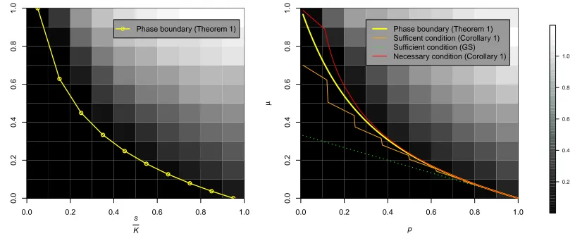
Contributions. There has not been much work on necessary conditions for local dictio-nary identifiability. Numerical experiments demonstrate that local identifiability undergoes a phase transition (Figure 1; see also Figure 3 of GS). The bound implied by the sufficient condition in GS falls well below the empirical phase boundary. Thus, even though theoret-ical results for the more general scenarios are available, we adopt the noiseless signals and complete dictionary setting of GS in order to find better local identifiability conditions. We summarize our main contributions below:
• For the population case whereN =∞, we establish a sufficient and almost necessary
condition for local identifiability under both thes-sparse Gaussian and the
Bernoulli-Gaussian models. For the Bernoulli-Bernoulli-Gaussian model, the phase boundary implied by our condition significantly improves the GS bound and agrees well with the empirical phase boundary (Figure 1).
• We provide lower and upper bounds to approximate the quantities in our local
iden-tifiability condition, as it generally requires to solve a series of second-order cone programs to compute those quantities.
• As a consequence, we show that aµ-coherent reference dictionary—a dictionary with
absolute pairwise column inner-product at most µ∈[0,1)—is locally identifiable for
sparsity level, measured by the average number of nonzeros in the random linear
coef-ficient vectors, up to the orderO(µ−2). Moreover, if the sparsity level is greater than
O(µ−2), the reference dictionary is generally not locally identifiable. In comparison,
the sufficient condition by GS demands the number of dictionary atomsK =O(µ−2),
which is a much more stringent requirement. For over-complete dictionaries, Geng
et al. (2011) requires the sparsity level to be of the order O(µ−1). It should also be
noted that Schnass (2015) establishes the bound O(µ−2) for approximatelocal
iden-tifiability under a new response maximization formulation of dictionary learning. To
the best of our knowledge, our result is the first in showing that O(µ−2) is achievable
and optimal for exact local recovery under the `1-minimization criterion.
• We also extend our identifiability results to the finite sample case. We show that for
a fixed sparsity level, we need N =O(KlogK) i.i.d. signals to determine whether or
not the reference dictionary can be identified locally. This sample requirement is the same as GS’s and is the best known sample requirement among all previous studies on local identifiability.
Other related works. Apart from analyzing the local minima of dictionary learning, another line of research aims at designing provable algorithms for recovering the reference dictionary. Georgiev et al. (2005) and Aharon et al. (2006a) proposed combinatorial algo-rithms and gave deterministic conditions for dictionary recovery which require sample size
N to be exponentially large in the number of dictionary atoms K. Spielman et al. (2012)
0.0 0.2 0.4 0.6 0.8 1.0
0.0
0.2
0.4
0.6
0.8
1.0
s
K
µ
●
●
●
●
●
●
● ●
● ●
o Phase boundary (Theorem 1)
0.0 0.2 0.4 0.6 0.8 1.0
0.0
0.2
0.4
0.6
0.8
1.0
p
µ
Phase boundary (Theorem 1) Sufficent condition (Corollary 1) Sufficient condition (GS) Necessary condition (Corollary 1)
0.2 0.4 0.6 0.8 1.0
Figure 1: Local recovery errors for thes-sparse Gaussian model (Left) and the Bernoulli(p
)-Gaussian model (Right). Under the s-sparse Gaussian model, the parameter
s∈ {1, . . . , K} is the number of nonzeros in each linear coefficient vector. Under
the Bernoulli(p)-Gaussian model, p ∈ (0,1] is the probability of an entry of the
linear coefficient vector being nonzero. The data are generated with the
refer-ence dictionaryD0 ∈R10×10 (i.e., K = 10) satisfying DT0D0 =µ11T + (1−µ)I
for µ ∈ [0,1), see Example 5 for details. For each (µ,Ks) or (µ, p) tuple, ten
batches of N = 2000 signals {xi}2000i=1 are generated according to the noiseless
linear model xi = D0αααi, with {αααi}2000i=1 drawn i.i.d. from the s-sparse Gaussian
model or i.i.d. from the Bernoulli(p)-Gaussian model. For each batch, the
dic-tionary is estimated through an alternating minimization algorithm in theSPAMS
package (Mairal et al., 2010), with initial dictionary set to beD0. The grayscale
intensity in the figure corresponds to the Frobenius error of the difference between
the estimated dictionary and the reference dictionary D0, averaged for the ten
batches. The “phase boundary” curve corresponds to the theoretical boundary that separates the region of local identifiability (below the curve) and the region of local non-identifiability (above the curve) according to Theorem 1 of this paper. The “Sufficient condition (Corollary 1)” and “Necessary condition (Corollary 1)” curves are the lower and upper bounds given by Corollary 1 to approximate the exact phase boundary. Finally, the “Sufficient condition (GS)” curve corresponds
to the lower bound by GS. Note that for thes-sparse Gaussian model, the
“Suf-ficient condition (Corollary 1)” and “Necessary condition (Corollary 1)” curves coincide with the phase boundary. See also Appendix Figures B.1 and B.2 for
recovers a complete reference dictionary for sparsity level up toO(K). While in this paper we do not provide an algorithm, our identifiability conditions suggest theoretical limits of dictionary recovery for all algorithms attempting to solve the optimization problem (2). In particular, in the regime where the reference dictionary is not identifiable, no algorithm can simultaneously solve (2) and recover the ground truth reference dictionary.
Other related works include generalization bounds for signal reconstruction errors under the learned dictionary (Maurer and Pontil, 2010; Vainsencher et al., 2011; Mehta and Gray, 2013; Gribonval et al., 2013), dictionary identifiability through combinatorial matrix theory (Hillar and Sommer, 2015), as well as algorithms and theories for the closely related inde-pendent component analysis (Comon, 1994; Arora et al., 2012b) and nonnegative matrix factorization (Arora et al., 2012a; Recht et al., 2012).
The rest of the paper is organized as follows: In Section 2, we give basic assumptions and describe the two probabilistic models for signal generation. Section 3 develops sufficient and almost necessary local identifiability conditions under both models for the population problem, and establishes lower and upper approximating bounds. In Section 4, we will present local identifiability results for the finite sample problem. Detailed proofs for the theoretical results can be found in the Appendix.
2. Preliminaries
In this section, we will introduce notations and basic assumptions for our analysis.
2.1 Notations
For a positive integerm, defineJmKto be the set of the firstmpositive integers,{1, . . . , m}.
The notation x[i] denotes thei-th entry of the vectorx∈Rm. For a non-empty index set
S ⊂JmK, we denote by |S|the set cardinality andx[S]∈R|S|the sub-vector indexed byS.
We definex[−j] := (x[1], . . . ,x[j−1],x[j+ 1], . . . ,x[m])∈Rm−1 to be the vectorxwithout
its j-th entry.
For a matrix A ∈ Rm×n, we denote by A[i, j] its (i, j)-th entry. For non-empty sets
S ⊂JmKand T ⊂JnK, denote by A[S, T] the sub-matrix of A with the rows indexed byS
and columns indexed byT. Denote byA[i,] andA[, j] the i-th row and thej-th column of
A respectively. Similar to the vector case, the notation A[−i, j]∈Rm−1 denotes the j-th
column of A without itsi-th entry.
For p ≥1, the `p-norm of a vector x∈Rm is defined as kxkp = (Pmi=1|x[i]|p)1/p, with
the convention that kxk0 =|{i: x[i]6= 0}| and kxk∞ = maxi|x[i]|. For any norm k.k on
Rm, the dual norm of k.k is defined as kxk∗ = supy6=0
xTy
kyk.
For two sequences of real numbers {an}∞n=1 and {bn}∞n=1, we denote by an = O(bn) if
there is a constantC >0 such that an≤Cbn for all n≥1. For a∈R, denote bybac the
integer part of a and dae the smallest integer greater than or equal toa. Throughout this
paper, we shall agree that 00 = 0.
2.2 Basic Assumptions
We denote byD ⊂Rd×K the constraint set of dictionaries for the optimization problem (2).
be theoblique manifold (Absil et al., 2008):
D=
D∈RK×K : kD[, k]k
2 = 1 for allk= 1, . . . , K .
We also call a dictionary column D[, k] an atomof the dictionary. Denote by D0 ∈ D
thereference dictionary, i.e., the ground truth dictionary that generates the signals. With these notations, we now give a formal definition for local identifiability:
Definition 1 (Local identifiability) Let L(D) : D → R be an objective function. We say that the reference dictionary D0 is locally identifiable with respect to L(D) ifD0 is a strict local minimum of L(D).
Sign-permutation ambiguity. As noted by previous works GS and Geng et al. (2011),
the `1-norm objective function L(D) = LN(D) of (2) has an intrinsic sign-permutation
ambiguity. LetD0=DPΛfor some permutation matrixPand diagonal matrixΛwith±1
diagonal entries. It is easy to see thatD0 and D have the same objective value. Thus, the
objective functionLN(D) has at least 2KK! local minima. We can only recoverD0 up to
column permutation and sign changes.
Note that if the dictionary atoms are linearly dependent, the effective dimension is
strictly less than K and the problem essentially becomes over-complete. Since dealing
with over-complete dictionaries is beyond the scope of this paper, we make the following assumption:
Assumption I (Complete dictionaries). The reference dictionary D0 ∈ D ⊂RK×K is
full rank.
Let M0 = DT0D0 be the dictionary atom collinearity matrix containing the
inner-products between dictionary atoms. Since each dictionary atom has unit`2-norm,M0[i, i] =
1 for all i∈JKK. In addition, as D0 is full rank, M0 is positive definite and |M0[i, j]|<1
for all i6=j.
We assume that a signal is generated as a random linear combination of the dictionary atoms. In this paper, we consider the following two probabilistic models for the random linear coefficients:
Probabilistic models for sparse coefficients. Denote byz ∈RK a random vector
from the K-dimensional standard normal distribution.
Model 1—SG(s). LetSbe a size-ssubset uniformly drawn from all size-ssubsets ofJKK.
Defineξξξ∈ {0,1}K by settingξξξ[j] =I{j∈S} forj∈
JKK, whereI{.}is the indicator
function. Letααα ∈RK be such thatααα[j] =ξξξ[j]z[j]. Then we sayααα is drawn from the
s-sparse Gaussian model, orSG(s).
Model 2—BG(p). Forj ∈JKK, letξξξ[j]’s bei.i.d. Bernoulli random variable with success
probability p ∈ (0,1]. Let ααα ∈ RK be such that ααα[j] = ξξξ[j]z[j]. Then we say ααα is
drawn from theBernoulli(p)-Gaussian model, orBG(p).
Assumption II (Signal generation). For i∈JNK, letαααi ∈RK be eitheri.i.d. s-sparse
Gaussian vectors ori.i.d.Bernoulli(p)-Gaussian vectors. The signalsxi ∈RK are generated
according to the noiseless linear model:
xi=D0αααi.
Remarks:
(1) The above two models and their variants were studied in a number of prior theoretical works, including Gribonval and Schnass (2010); Geng et al. (2011); Agarwal et al. (2014b); Sun et al. (2017).
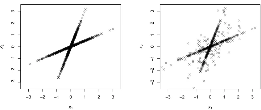
(2) By construction, a random vector generated from the s-sparse model has exactly s
nonzero entries. The data points xi’s therefore lie within the union of the linear spans of
s dictionary atoms (Figure 2 Left). The Bernoulli(p)-Gaussian model, on the other hand,
allows the random coefficient vector to have any number of nonzero entries ranging from 0
toK with a mean ofpK. As a result, some data points, called “non-sparse outliers” in GS,
can be outside of any sparse linear span of the dictionary atoms (Figure 2 Right and Figure 1 of GS). We refer readers to the remarks following Example 5 in Section 3 for a discussion of the effect of non-sparse outliers on local identifiability.
(3) Gribonval et al. (2015) assumed a more general distribution for the sparse coefficients. While our local identifiability results can potentially be extended to their model, such an extension would require significantly more complicated notations and make the correspond-ing results less interpretable. For the sake of accessibility and interpretability, we focus only on the two probabilistic models above.
In this paper, we study the problem of dictionary identifiability with respect to the
population objective functionELN(D) (Section 3) and the finite sample objective function
LN(D) (Section 4). In order to analyze these objective functions, it is convenient to define
the following “group LASSO”-type norms:
Definition 2 Let m≥1 be an integer andw∈Rm.
1. For k∈JmK, define
|||w|||k =
P
|S|=kkw[S]k2
m−1
k−1
.
2. For p∈(0,1), define
|||w|||p =
m−1
X
k=0
pbinom(k;m−1, p)|||w|||k+1,
where pbinom is the probability mass function of the binomial distribution:
pbinom(k;n, p) =
n k
pk(1−p)n−k.
Remarks:
−3 −2 −1 0 1 2 3
−3
−2
−1
0
1
2
3
x1 x2
−3 −2 −1 0 1 2 3
−3
−2
−1
0
1
2
3
x1 x2
Figure 2: Data generation forK = 2. Left: thes-sparse Gaussian model withs= 1; Right:
the Bernoulli(p)-Gaussian model with p = 0.2. The inner product between the
two dictionary atoms is 0.7. A sample ofN = 1000 data points are generated for
both models. For thes-sparse model, all data points are perfectly aligned with
the two lines corresponding to the two dictionary atoms. For the Bernoulli(p
)-Gaussian model, a number of data points fall outside the two lines. According to our Theorem 1 and 3, despite those outliers and the high collinearity between
the two atoms, the reference dictionary is still locally identifiable forN =∞ and
with high probability for finite samples.
with the random vectorαααdrawn fromSG(s) andBG(p) models respectively. For invertible
D∈ D, it can be shown that the objective function for one signalx=D0ααα is
l(x,D) =kHαααk1=
K
X
j=1
|H[j,]ααα|,
whereH=D−1D0. Thus, taking the expectation of the objective function with respect to
x, we end up with a quantity involving either PK
j=1|||H[j,]|||s or
PK
j=1|||H[j,]|||p. This is
the motivation of defining these norms.
(2) In particular, |||w|||1 =kwk1 and|||w|||m=kwk2.
(3) The norms defined above are special cases of the group LASSO penalty by Yuan and
Lin (2006). For |||w|||k, the summation covers all size-k subsets of JmK. The normalization
factor is the number of times w[i] appears in the numerator. Thus, |||w|||k is essentially
the average of the `2-norms of all size-k sub-vectors of w. On the other hand, |||w|||p is a
3. Population Analysis
In this section, we establish local identifiability results for the case where infinitely many
sig-nals are observed. Denote byEl(x1,D) the expectation of the objective functionl(x1,D) of
(1) with respect to the random signalx1. By the strong law of large numbers, as the number
of signals N tends to infinity, the empirical objective function LN(D) = N1
PN
i=1l(xi,D)
converges almost surely to its population meanEl(x1,D) for each fixedD∈ D. Therefore
the population version of the optimization problem (2) is
min
D∈D E l(x1,D) (3)
Since by assumption the reference dictionary D0 is full rank, we only need to work with
D ∈ D that is also full rank. Indeed, if the linear span of columns span(D) 6= RK, then
D0ααα1 6∈ span(D) with nonzero probability. Thus D is infeasible with nonzero probability
and so E l(x1,D) = +∞. For a full rank dictionary D, the following lemma gives the
closed-form expression for the expected objective function El(x1,D).
Lemma 1 (Closed-form objective functions) Let Dbe a full rank dictionary in Dandx1= D0ααα1, where ααα1∈RK is a random vector. For notational convenience, let H=D−1D0.
1. Ifααα1 is generated according to the SG(s) model withs∈JK−1K,
LSG(s)(D) :=El(x1,D) =
r
2
π s K
K
X
j=1
|||H[j,]|||s. (4)
2. Ifααα1 is generated according to the BG(p) model withp∈(0,1),
LBG(p)(D) :=El(x1,D) =
r
2
πp
K
X
j=1
|||H[j,]|||p. (5)
For the non-sparse cases where s=K and p= 1, we have
LSG(s)(D) =LBG(p)(D) =
r
2
π
K
X
j=1
kH[j,]k2.
Remarks: It can be seen from the above closed-form expressions that the two models are
closely related. First of all, it is natural to identifypwithKs, the fraction of expected number
of nonzero entries inααα1. Next, by definition,|||.|||p is a binomial average of |||.|||k. Therefore,
the Bernoulli-Gaussian objective functionLBG(p)(D) can be treated as a binomial average
of the s-sparse objective function LSG(s)(D).
By analyzing the above closed-form expressions of the `1-norm objective function, we
Theorem 1 (Population local identifiability) Recall that M0 = DT0D0 and M0[−j, j]
de-notes the j-th column of the off-diagonal part of M0. Let|||.|||∗s and |||.|||∗p be the dual norm of |||.|||s and |||.|||p respectively.
1. (SG(s) models) ForK ≥2 and s∈JK−1K, if
max
j∈JKK
|||M0[−j, j]|||∗s <1− s−1
K−1.
thenD0 is locally identifiable with respect to LSG(s).
2. (BG(p) models) ForK ≥2 and p∈(0,1), if
max
j∈JKK
|||M0[−j, j]|||∗p <1−p.
thenD0 is locally identifiable with respect to LBG(p).
Moreover, the above conditions are almost necessary in the sense that if the reversed strict inequalities hold, then D0 is not locally identifiable.
On the other hand, if s=K or p= 1, then D0 is not locally identifiable with respect to
LSG(s) or LBG(p).
Proof sketch. Let {Dt}t∈R be a collection of dictionaries Dt ∈ D indexed by t ∈ R
and L(D) =El(x1,D) be the population objective function. The reference dictionaryD0
is a strict local minimum of L(D) on the manifoldDif and only if the following statement
holds: for any {Dt}t∈R that is a smooth function of t with non-vanishing derivative at
t = 0, L(Dt) has a strict local minimum at t = 0. For a fixed {Dt}t∈R, to ensure that
L(Dt) achieves a strict local minimum at t= 0, it suffices to have the following one-sided
derivative inequalities:
lim
t↓0+
L(Dt)−L(D0)
t >0 and limt↑0−
L(Dt)−L(D0)
t <0.
It can be shown that the above inequalities are equivalent to:
max
j∈JKK
M0[−j, j]
Tw
<
1− s−1
K−1 forSG(s)
1−p forBG(p)
wherew∈RK−1 is a unit vector under norm|||.|||s or|||.|||p and corresponds to the direction
in whichDt approachesD0 asttends to zero. Sincet= 0 has to be a strict local minimum
for all smooth {Dt}t∈R or approaching directions, by taking the supremum over all such
unit vectors the LHS of the above inequality becomes the dual norm of|||.|||sor|||.|||p. On the
other hand,D0 is not a local minimum if limt↓0+(L(Dt)−L(D0))/t <0 or limt↑0−(L(Dt)−
L(D0))/t >0 for some{Dt}t∈R. Thus the sufficient condition is also almost necessary. We
refer readers to Section A.1.2 for the detailed proof.
Local identifiability phase boundary. Theorem 1 indicates that population local identifiability undergoes a phase transition. The following equations
max
j∈JKK
|||M0[−j, j]|||∗s = 1− s−1
K−1 and maxj∈JKK
define the phase boundaries which separate the regions of local identifiability and
non-identifiability under respective models. It is unclear whether D0 is locally identifiable on
the phase boundary. If either equality in (6) holds, the directional derivative of the objective
function at D0 become zero in certain directions. Hence analyzing local identifiability in
this case requires higher order derivative computations that quickly become complicated.
Collinearity and sparsity. These are the two factors that determine local
identifi-ability. Intuitively, for D0 to be locally identifiable, neither can the atoms of D0 be too
linearly dependent, nor can the random linear coefficients be too dense. For the s-sparse
Gaussian model, the quantity maxj∈JKK|||M0[−j, j]|||
∗
s measures the size of the off-diagonal
entries ofM0 and hence the collinearity of the dictionary atoms. In addition, that quantity
depends on the sparsity parameters. By Lemma 7 in the Appendix, maxj∈JKK|||M0[−j, j]|||
∗
s
is increasing with respect to s. Similar conclusion holds for the Bernoulli-Gaussian model.
Therefore, sparser linear coefficients will lead to less restrictive requirement on dictionary atom collinearity. See, for example, the phase boundaries in Figure 1.
Next, we will present a few examples to gain more intuition for the local identifiability conditions.
Example 1 (1-sparse Gaussian model) A full rank D0 is always locally identifiable at the
population level under a 1-sparse Gaussian model. Indeed, by Corollary 7 in the Appendix,
|||M0[−j, j]|||∗1 = maxi6=j|M0[i, j]| < 1 for all j ∈ JKK. Thus, a full rank dictionary D0
always satisfies the sufficient condition.
Example 2 ((K−1)-sparse Gaussian model) For j∈JKK, by Corollary 7, |||M0[−j, j]|||∗K−1 =kM0[−j, j]k2.
Therefore the phase boundary under the (K−1)-sparse model is
max
j∈JKK
kM0[−j, j]k2=
1
K−1.
Example 3 (Orthogonal dictionaries) If M0 =I, then
max
j∈JKK
|||M0[−j, j]|||∗s= max j∈JKK
|||M0[−j, j]|||∗p = 0.
Therefore orthogonal dictionaries are always locally identifiable if s < K or p <1.
Example 4 (Minimally dependent dictionary atoms) Let µ ∈ (−1,1). Consider a dictio-nary atom collinearity matrix M0 such that M0[1,2] = M0[2,1] = µ and M0[i, j] = 0 for
all other i6=j. By Corollary 8,
max
j∈JKK
|||M0[−j, j]|||∗s = max
j∈JKK
|||M0[−j, j]|||∗p=|µ|.
Thus the phase boundaries under respective models are
|µ|= 1− s−1
K−1 and |µ|= 1−p.
Example 5 (Constant inner-product dictionaries) LetM0 =µ11T+(1−µ)I, i.e.,D0[, i]TD0[, j] =
µ for 1 ≤i < j ≤ K. Note that M0 is positive definite if and only if µ∈ (−K1−1,1). By Corollary 9, we have
|||M0[−j, j]|||∗s=
√
s|µ|.
Thus for the s-sparse model, the phase boundary is
√
s|µ|= 1− s−1
K−1.
Similarly for the Bernoulli(p)-Gaussian model, we have
|||M0[−j, j]|||∗p =|µ|p(K−1)
KX−1
k=0
pbinom(k, K−1, p)
√
k
−1
.
Thus the phase boundary is
|µ|= 1−p
p(K−1)
K−1
X
k=0
pbinom(k, K−1, p)
√
k.
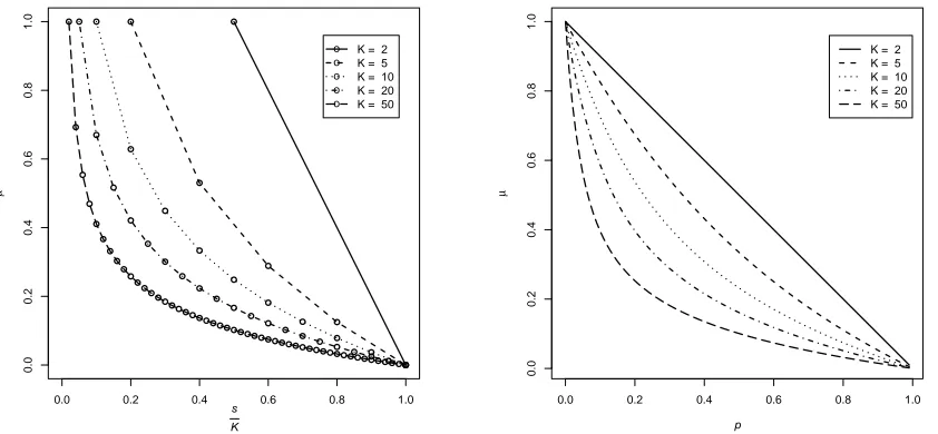
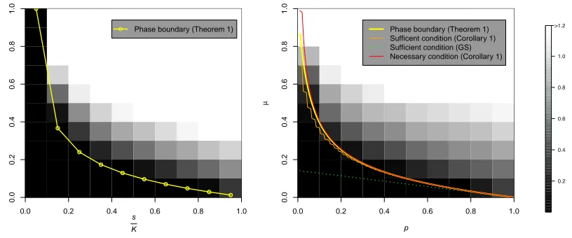
Figures 3 shows the phase boundaries for different dictionary sizes under the two models. As K increases, the phase boundary moves toward the lower left of the region. This observation indicates that recovering the reference dictionary locally becomes increasingly difficult for larger dictionary size. See also Appendix Figures B.1 and B.2 for simulation results with larger K’s.
The effect of non-sparse outliers. Example 5 demonstrates how the presence of non-sparse outliers in the Bernoulli-Gaussian model (Figure 2 Right) affects the requirements
for local identifiability. Setp= Ks in order to have the same level of sparsity with theSG(s)
model. Applying Jensen’s inequality, one can show that
1−p
p(K−1)
K−1
X
k=0
pbinom(k, K−1, p)
√
k < √1
s(1− s−1
K−1),
which indicates that the phase boundary of thes-sparse models is always above that of the
Bernoulli-Gaussian model with the same level of sparsity. The gap between the two phase
boundaries is the extra cost in terms of the collinearity parameterµ for locally recovering
the dictionary in the presence of non-sparse outliers. One extreme example is the case
where s = 1 and correspondingly p = K1. By Example 1, under a 1-sparse model the
reference dictionary D0 is always locally identifiable if|µ|<1. But for theBG(K1) model,
by the remarks under Corollary 1, D0 is not locally identifiable if |µ|>1−K1. Hence, the
requirement for µin the presence of outliers is at least K1 more stringent than that in the
case of no outliers.
However, such a difference diminishes as the number of dictionary atoms K increases.
Indeed, by Lemma 2, one can establish the following lower bound for the phase boundary
under the BG(p) model
1−p
p(K−1)
K−1
X
k=0
pbinom(k, K−1, p)√k≥ p 1−p
p(K−1) + 1 ≈
1
√
s(1− s−1
0.0 0.2 0.4 0.6 0.8 1.0
0.0
0.2
0.4
0.6
0.8
1.0
s K
µ
●
● ●
●
●
●
● ●
●
●
●
●
●
●
●
● ● ●
●
●
●
●
● ●
● ●
● ●
● ●
●
● ●
● ●
● ●
●
●
●
●
●
● ●
● ●
●
●●
●●
●●● ●
● ●● ●
● ● ●● ● ●
● ● ● ●● ● ● ●
● ● ● ● ●● ● ● ● ● ●
● ● ●
o o o o o
K = 2 K = 5 K = 10 K = 20 K = 50
0.0 0.2 0.4 0.6 0.8 1.0
0.0
0.2
0.4
0.6
0.8
1.0
p
µ
K = 2 K = 5 K = 10 K = 20 K = 50
Figure 3: Local identifiability phase boundaries for constant inner-product dictionaries,
un-der Left: the s-sparse Gaussian model; Right: the Bernoulli(p)-Gaussian model.
For each model, phase boundaries for different dictionary sizesKare shown. Note
that Ks ∈ {1
K,
2
K, . . . ,1} and p ∈(0,1]. The area under the curves is the region
where the reference dictionaries are locally identifiable at the population level.
Due to symmetry, we only plot the portion of the phase boundaries forµ >0.
for fixed sparsity levelp= Ks and large K.
In general, the dual norms |||.|||∗s and |||.|||∗p have no closed-form expressions. According
to Corollary 6 in the Appendix, computing those quantities involves solving a second order cone problem (SOCP) with exponentially many constraints. The following Lemma 2, on the other hand, gives computationally inexpensive approximation bounds.
Definition 3 (Hyper-geometric distribution related quantities) Let m be a positive integer andd, k ∈ {0}∪JmK. Denote byLm(d, k)the hypergeometric random variable with parameter
m, d and k, i.e., the number of 1’s after drawing without replacement k elements from d 1’s and m−d 0’s. Now for each d∈ {0} ∪JmK, define the function τm(d, .) with domain
on[0, m]as follows: set τm(d,0) = 0. For a∈(k−1, k] where k∈JmK, define
τm(d, a) =EpLm(d, k−1) + (EpLm(d, k)−EpLm(d, k−1))(a−(k−1)).
Lemma 2 (Lower and upper bounds for |||.|||∗s and |||.|||∗p) Let m be a positive integer and
z∈Rm.
1. For s∈JmK,
max kzk∞,
r
s mTmax⊂JmK
kz[T]k1
p |T|
!
≤ s
mTmax⊂JmK
kz[T]k1
τm(|T|, s)
≤ |||z|||∗s≤ max
2. For p∈(0,1),
max kzk∞,√p max
T⊂JmK
kz[T]k1 p
|T| !
≤p max
T⊂JmK
kz[T]k1
τm(|T|, pm)
≤ |||z|||∗p ≤ max
S⊂JmK,|S|=k
kz[S]k2.
where k=dp(m−1) + 1e.
Remarks:
(1) We refer readers to Lemma 10 and 11 for the detailed version of the above results.
(2) Since we agree that 00 = 0, the case where T =∅ does not affect taking the maximum
of all subsets.
(3) Consider a sparse vector z= (z,0, . . . ,0)T ∈Rm. By Corollary 8,
|||z|||∗s =|||z|||∗p =|z|=kzk∞= max
S⊂JmK,|S|=1
kz[S]k2.
So the all the bounds are achievable by a sparse vector.
(4) Now consider a dense vector z= (z, . . . , z)T ∈Rm. By Corollary 9,
|||z|||∗s=√s|z|=
r
s mTmax⊂JmK
kz[T]k1
p
|T| =S⊂JmaxmK,|S|=skz[S]k2.
Thus the bounds for|||z|||∗s can also be achieved by a dense vector. Similarly, by the
upper-bound for|||z|||∗p,
|||z|||∗p ≤ppm+ 1|z|.
On the other hand,
|||z|||∗p ≥√p max
T⊂JmK
kzk1
p
|T|=
√
p|z| max
T⊂JmK
p
|T|=√pm|z|.
Thus both bounds for|||z|||∗p are basically the same for large pm.
(5) Computation. To compute the lower and upper bounds efficiently, we first sort the
elements in|z|in descending order. Without loss of generality, we can assume that|z[1]| ≥
|z[2]| ≥. . .≥ |z[m]|. Thus the upper-bound quantity becomes
max
S⊂JmK,|S|=k
kz[S]k2 = (
k
X
i=1
z[i]2)1/2.
For the lower-bound quantities, note that
max
T⊂JmK
kz[T]k1
τm(|T|, k)
= max
d∈JmK
max
T⊂JmK,|T|=d
kz[T]k1
τm(d, k)
= max
d∈JmK
Pd
i=1|z[i]|
τm(d, k)
.
Thus, the major computation burden now is τm(d, k) = EpLm(d, k), for alld∈JmK. We
do not know a closed-form formula forEpLm(d, k) except ford= 1 ord=m. In practice,
we compute EpLm(d, k) using its definition formula. On an OS X laptop with 1.8 GHz
R can compute EpL2000(d,1000) for all d ∈ J2000K within 0.635 second. Note that the
number of dictionary atoms in most applications is typically smaller than 2000.
When m is too large, the LHS lower bounds can be used. Note that
max
T⊂JmK
kz[T]k1
p
|T| = maxd∈JmK
Pd
i=1√|z[i]|
d ,
which can be computed easily.
For notational simplicity, we will define the following quantities:
Definition 4 For a∈(0, K), define
νa(M0) = max
1≤j≤KS⊂maxJKK,j6∈S
kM0[S, j]k1
τK−1(|S|, a)
.
Definition 5 (Cumulative coherence) Fork∈JK−1K, define thek-th cumulative coherence of a reference dictionaryD0 as
µk(M0) = max
1≤j≤KS⊂JKKmax,|S|=k,j6∈S
kM0[S, j]k2.
Remarks: The above quantity is actually the`2analog of the`1 k-th cumulative coherence
defined in Gribonval et al. (2015). Also, notice that µ1(M0) = maxl=6 j|M0[l, j]| which is
the plain mutual coherence of the reference dictionary.
With the above definitions and as a direct consequence of Lemma 2, we obtain a sufficient condition and a necessary condition for population local identifiability:
Corollary 1 Under the notations of Theorem 1, we have
1. Let K≥2 and s∈JK−1K.
• If µs(M0)<1−Ks−−11, then D0 is locally identifiable with respect to LSG(s);
• If Ks−1νs(M0)>1−Ks−−11, then D0 is not locally identifiable with respect to LSG(s).
2. Let K≥2 and p∈(0,1).
• If µk(M0) < 1−p, where k = dp(K −2) + 1e, then D0 is locally identifiable with
respect to LBG(p);
• Ifpνk(M0)>1−p, wherek=p(K−1), thenD0 is not locally identifiable with respect
to LBG(p). Remarks:
(1) In particular, by Lemma 2, if µ1(M0) >1− Ks−−11 or µ1(M0) > 1−p, then D0 is not
locally identifiable.
(2) We can also replace Ks−1νs(M0) orpνk(M0) by the corresponding lower bound quantities
Comparison with GS. Corollary 1 enables us to compare our local identifiability
condition directly with that of GS. For the Bernoulli(p)-Gaussian model, the population
version of the sufficient condition for local identifiability by GS is:
µK−1(M0) = max
1≤j≤KkM0[−j, j]k2<1−p. (7)
Note thatµK−1(M0)≥µk(M0) for k≤K−1.
Thus, our local identifiability result implies that of GS. Moreover, the quantitykM0[−j, j]k2
in inequality (7) computes the`2-norm of the entireM0[−j, j] vector and is independent of
the sparsity parameterp. On the other hand, in our sufficient condition, max|S|=k,j6∈SkM0[S, j]k2
computes the largest`2-norm of all size-ksub-vectors ofM0[−j, j]. Sincek=dp(K−2) + 1e
is essentially pK, when the random linear coefficients are sparse, the sufficient bound by
GS is much more conservative compared to ours.
More concretely, let us consider constant inner-product dictionaries with parameter
µ > 0 as in Example 5. The sufficient conditions by GS and by our Corollary 1 are
respectively √
Kµ≤1−p and ppK+ 1µ≤1−p,
showing that the sufficient condition by GS is much more conservative for small value ofp.
See Figure 1, Appendix Figures B.1 and B.2 for a graphical comparison of the bounds for
K = 10,20 and 50.
Local identifiability for sparsity level O(µ−2). For notational convenience, let
µ=µ1(M0) be the mutual coherence of the reference dictionary. For thes-sparse model,
by Lemma 2,µs(M0)≤
√
sµ. Thus the first part of the corollary implies a simpler sufficient
condition:
√
sµ <1− s−1
K−1.
From the above inequality, it can be seen that if 1− s−1
K−1 > δfor some δ >0, the reference
dictionary is locally identifiable for sparsity level sup to the orderO(µ−2).
Similarly for the Bernoulli(p)-Gaussian model, since for k=dp(K−2) + 1e,
µk(M0)≤
p
pK+ 1µ,
we have the following sufficient condition for local identifiability:
p
pK+ 1µ≤1−p.
As before, if 1−p > δ for some δ > 0, the reference dictionary is locally identifiable for
sparsity level pK up to the order O(µ−2). On the other hand, the same arguments for the
condition by GS leads to K =O(µ−2), which, does not take advantage of sparsity.
In addition, by Example 5 and Remark (4) under Lemma 2, we also know that the
sparsity requirementO(µ−2) cannot be improved in general.
Our result seems to be the first to demonstrate that O(µ−2) is the optimal order of
sparsity level for exact local recovery of a reference dictionary. For a predefined
over-complete dictionary, classical results such as Donoho and Elad (2003) and Fuchs (2004)
up to the order O(µ−1). For over-complete dictionary learning, Geng et al. (2011) showed
that exact local recovery is also possible for s-sparse model with s up to O(µ−1). While
our results are only for complete dictionaries, we conjecture thatO(µ−2) is also the optimal
order of sparsity level for over-complete dictionaries. In fact, Schnass (2015) proved that the response maximization criterion—an alternative formulation of dictionary learning— can approximately recover the over-complete reference dictionary locally with sparsity level
sup toO(µ−2). It will be of interest to investigate whether the same sparsity requirement
hold for the `1-minimization dictionary learning (2) in the case of exact local recovery and
over-complete dictionaries.
A note on global identifiability. With the notations in Definition 1, we say that the
reference dictionary D0 is globally identifiable with respect to L(D) if (1) D0 is a global
minimum ofL(D), and (2) for any other dictionary D0 that cannot be transformed toD0
under any column permutation and sign changes, L(D0) < L(D0). It is easy to see that
global identifiability implies local identifiability, and so any necessary conditions for local identifiability are also necessary for global identifiability. Sufficient conditions for the global case are much harder to find. However, for dictionaries with orthogonal columns, we can show the following:
Corollary 2 Suppose that the reference dictionary D0 is orthogonal, i.e., M0=I.
1. D0 is globally identifiable with respect to LSG(s) if and only if Ks <1.
2. D0 is globally identifiable with respect to LBG(p) if and only if p <1.
The above result indicates that for orthogonal dictionaries, we have global identifiability
as long as the linear coefficientsαααi’s are not entirely dense. Note that these conditions are
exactly the same as in the local identifiability case, see Example 3. Naturally, it is of greater interest to derive global identifiability condition for non-orthogonal dictionaries. Simulation
results in Figure 3 of GS demonstrate that for K = 2, global identifiability seems to share
the same phase transition boundary with local identifiability, i.e., µ+p= 1. Furthermore,
the surface plot of the objective function in Figure 2 of GS shows no other spurious local minima. To establish global identifiability for non-orthogonal dictionaries, it is unavoidable to characterize global optima of the non-convex objective function. An on-going work of Y. Wang and the authors (Wang et al.) might help shed light on this challenging problem.
4. Finite Sample Analysis
In this section, we will present finite sample results for local dictionary identifiability. For notational convenience, we first define the following quantities:
P1(, N;µ, K) = 2 exp
− N
2
108Kµ
,
P2(, N;p, K) = 2 exp
−p N
2
18p2K+ 9√2pK
,
P3(, N;p, K) = 3
24
p + 1
K
exp
−pN
2
360
Recall thatM0=DT0D0andµ1(M0) is the mutual coherence of the reference dictionary
D0. The following two theorems give local identifiability conditions under the s-sparse
Gaussian model and the Bernoulli-Gaussian model:
Theorem 2 (Finite sample local identifiability for SG(s)) Let αααi ∈RK, i∈JNK, be i.i.d.
SG(s) random vectors with s ∈ JK −1K. The signals xi’s are generated as xi = D0αααi.
Assume 0< ≤ 1 2.
1. If
max
j∈JKK
|||M0[−j, j]|||∗s≤1−
s−1
K−1−
r
π
2,
thenD0 is locally identifiable with respect to LN(D) with probability exceeding
1−K2
P1(, N;µ1(M0), K) +P2(, N;
s
K, K) +P3(, N; s K, K)
.
2. If
max
j∈JKK
|||M0[−j, j]|||∗s≥1− s−1
K−1+
r
π
2,
thenD0 is not locally identifiable with respect to LN(D) with probability exceeding
1−KP1(, N;µ1(M0), K) +P2(, N;
s
K, K) +P3(, N; s K, K)
.
Theorem 3 (Finite sample local identifiability for BG(p)) Letαααi∈RK, i∈JNK, be i.i.d.
BG(p) random vectors with p ∈ (0,1). The signals xi’s are generated as xi = D0αααi. Let
Kp =K+ 2p−1 and assume 0< ≤ 12.
1. If
max
j∈JKK
|||M0[−j, j]|||∗p ≤1−p−
r
π
2,
thenD0 is locally identifiable with respect to LN(D) with probability exceeding
1−K2(P1(, N;µ1(M0), Kp) +P2(, N;p, Kp) +P3(, N;p, K)).
2. If
max
j∈JKK
|||M0[−j, j]|||∗p ≥1−p+
r
π
2,
thenD0 is not locally identifiable with respect to LN(D) with probability exceeding
1−K(P1(, N;µ1(M0), Kp) +P2(, N;p, Kp) +P3(, N;p, K)).
Remarks: The conditions for finite sample local identifiability are essentially identical to
their population counterparts. The main difference is an margin ofpπ
2on the RHS of the
inequalities. Such a margin appears as a result of our proof techniques: we show that the
derivative ofLN is within O() of its expectation and then apply local identifiability results
Sample size requirement. The theorems indicate that if the number of signals is a multiple of the following quantity,
ForSG(s): 1
2max
µ1(M0)KlogK, slogK,
K s Klog
K s
ForBG(p): 1
2max
µ1(M0)KlogK, pKlogK,
1
pKlog
1
p
then with high probability we can determine the conditions for local identifiability. Thus, in the worst case, the sample size requirements for the two models are respectively
O(Klogs K
K
) andO(KlogK
p ).
Our sample size requirement is similar to that of GS, who shows that O(Kp(1log−pK)) signals
is enough for locally recovering an incoherent reference dictionary. Our result indicates the
1−p factor in their denominator is not necessary.
The following two corollaries are the finite sample counterparts of Corollary 1.
Corollary 3 Under the same assumptions of Theorem 2,
1. (Sufficient condition for SG(s)) If
µs(M0)≤1−
s−1
K−1 −
r
π
2,
thenD0 is locally identifiable with respect to LN(D), with the same probability bound
in the first part of Theorem 2.
2. (Necessary condition for SG(s)) If
s
K−1νs(M0)≥1−
s−1
K−1 +
r
π
2,
then D0 is not locally identifiable with respect to LN(D), with the same probability
bound in the second part of Theorem 2.
Corollary 4 Under the same assumptions of Theorem 3,
1. (Sufficient condition for BG(p)) Let k=dp(K−1) + 1e. If
µk(M0)≤1−p−
r
π
2,
thenD0 is locally identifiable with respect to LN(D), with the same probability bound
2. (Necessary condition for BG(p)) Let k=p(K−1). If
pνk(M0)≥1−p+
r
π
2,
then D0 is not locally identifiable with respect to LN(D), with the same probability
bound in the second part of Theorem 3.
Remarks: As before, denote by µ∈ [0,1) the coherence of the reference dictionary. The above two corollaries indicate that the reference dictionary is locally identifiable with high
probability for sparsity levelsorpK up to the order O(µ−2).
Proof sketch for Theorem 2 and 3. Similar to the population case, by taking
one-sided derivatives ofLN(Dt) with respect totatt= 0 for all smooth{Dt}t∈R, we can derive
a sufficient and almost necessary algebraic condition for the reference dictionary D0 to be
a strict local minimum ofLN(D). Using the concentration inequalities in Lemma 3—5, we
show that the stochastic terms in the algebraic condition are close to their expectations with high probability. The population results for local identifiability can then be applied. The proofs for the two signal generation models are conceptually the same after establishing
Lemma 8 to relate the |||.|||∗p norm to the |||.|||∗s norm. The detailed proof can be found in
Section A.2.
Comparison with the proof by GS. The key difference between our analysis and that of GS is that we use an alternative but equivalent formulation of dictionary learning. Instead of (2), GS studied the following problem:
min D∈D,αααi
1
N
N
X
i=1
kαααik1 (8)
subject to xi =Dαααi for alli∈JNK.
Note that the above formulation optimizes jointly overDandαααifori∈JNK, as opposed
to optimizing with respect to the only parameterD in our case. For complete dictionaries,
this formulation is equivalent to the formulation in (2) in the sense that ˆDis a local minimum
of (2) if and only if ( ˆD,Dˆ−1[x1, . . . ,xN]) is a local minimum of (8), see Remark 3.1 of GS.
The number of parameters to be estimated in (8) is O(K2 +KN), compared to O(K2)
free parameters in (2). The growing number of parameters make the GS formulation less tractable to analyze under a signal generation model.
GS did not directly study the population case. They first obtained an algebraic condition for local identifiability that is sufficient and almost necessary. However, the condition is
convoluted and hard to interpret due to its direct dependence on the signals xi’s. In
order to determine the number of signals required for successful local recovery, they further investigated their condition under the Bernoulli-Gaussian model. During the probabilistic analysis, the sharp algebraic condition was weakened, resulting in a sufficient condition that is far from being necessary.
In contrast, we start with probabilistic generative models. The number of parameters
and to apply concentration inequalities for the finite sample problem. Therefore, studying the optimization problem (2) instead of (8) is the key to establishing an interpretable sufficient and almost necessary local identifiability condition.
5. Conclusions and Future Work
We have established sufficient and almost necessary conditions for local dictionary
identifia-bility under both thes-sparse Gaussian model and the Bernoulli-Gaussian model in the case
of noiseless signals and complete dictionaries. For finite samples with a fixed sparsity level,
we have shown that as long as the number of i.i.d.signals scales as O(KlogK), with high
probability we can determine the local identifiability conditions of a reference dictionary.
There are several directions for future research. In this paper, we focused mainly on the
local behaviors of the`1-norm objective function. As we previously discussed, investigating
global identifiability conditions is a natural next step. Simulations in GS suggest a close connection between local and global identifiability. To understand this problem further, we need to characterize global optima of the non-convex objective function. In an on-going work of Y. Wang and the authors, we are developing promising techniques to analyze global
properties of `1-minimization dictionary learning in the non-orthogonal case.
Moreover, one can extend our results to a wider class of sub-Gaussian distributions other than the standard Gaussian distribution considered in this paper. We foresee little technical difficulty for this extension. However, it should be noted that the quantities
in-volved in our local identifiability conditions, i.e., the|||.|||∗sand|||.|||∗pnorms, are consequences
of the standard Gaussian assumption. Under a different distribution, it can be even more computationally challenging to verify the resulting local identifiability conditions.
Finally, it would be also desirable to improve the sufficient condition by Geng et al. (2011) and Gribonval et al. (2015) for over-complete dictionaries and noisy signals. One interesting implication of our results is that local recovery is possible for sparsity level up
to the orderO(µ−2) for a µ-coherent reference dictionary. We conjecture the same sparsity
requirement for the over-complete and/or noisy signal cases. In either scenario, the closed-form expression for the objective function is no longer available. A full characterization of local dictionary identifiability demands novel techniques for analyzing the local behaviors of the objective function.
Acknowledgments
Appendix A. Proofs
Let L(D) be the dictionary learning objective function and {Dt}t∈R be the collection of
dictionaries Dt ∈ D parameterized by t ∈ R. By definition, {Dt}t∈R passes through the
reference dictionary D0 at t= 0. Similar to Gribonval and Schnass (2010), to ensure that
D0 is a strict local minimum ofL(D), it suffices to have
lim
t↓0+
L(Dt)−L(D0)
t >0 and limt↑0−
L(Dt)−L(D0)
t <0,
for all {Dt}t∈R that is a smooth function of t with rate of approaching D0 bounded away
from zero. On the other hand, if either of the above strict inequalities holds in the reversed
direction for some smooth{Dt}t∈R, thenD0 is not a local minimum of L(D).
Since D0 is full rank by assumption, the minimum eigenvalue ofM0=DT0D0 is strictly
greater than zero. By continuity of the minimum eigenvalue of DTtDt(see e.g., the
Bauer-Fike Theorem), Dt should also be full rank whent is sufficiently small. Thus without loss
of generality we can only consider full rank dictionariesDt. For any full rankD∈ D, there
is an invertible matrixA∈RK×K such thatD=D0A. For anyk∈JKK, by the constraint
kD[, k]k2 = 1,A[, k]TM0A[, k] = 1. Define the set for all suchA’s as
A={A∈RK×K :A is invertible and A[, k]TM0A[, k] = 1 for all k∈JKK}. (9)
It follows immediately that the set {D0A:A∈ A}is the collection ofD∈ D such that D
is full rank. Thus, to ensure that D0 is a strict local minimum ofL(D), it suffices to show
∆+(L,{At}t) := lim
t↓0+
L(D0At)−L(D0)
t >0, (10)
∆−(L,{At}t) := lim
t↑0−
L(D0At)−L(D0)
t <0, (11)
for all smooth functions{At}t∈R with At∈ A,A0 =I and nonzero derivative att= 0. In
addition, to demonstrate that D0 is not a local minimum of L(D), it suffices to have (10)
or (11) to hold in the reversed direction for some{At}twith the aforementioned properties.
We will be using this characterization of local minimum to prove local identifiability results for both the population case and the finite sample case.
A.1 Proofs of the Population Results
A.1.1 Proof of Lemma 1
Proof SinceE||Hααα1||1=PKj=1E|H[j,]ααα1|, it suffices to computeE|H[j,]ααα1|. LetSbe any
nonempty subset ofJKK. Recall that the random variableS1 ⊂JKKdenotes the support of
random coefficient ααα1. Conditioning on the event{S1 =S}, the random variable H[j,]ααα1
follows a normal distribution with mean 0 and standard deviationkH[j, S]k2. Hence
E|H[j,]ααα1|=E[E[|H[j,]ααα1| |S1]] =
r
2
(1) Under the s-sparse Gaussian model,P(S1 =S) = Ks
−1
for any |S|=s. Thus we have
EkH[j,S1]k2=
K s
−1
X
S:|S|=s
kH[j, S]k2 = s
K|||H[j,]|||s.
Hence the objective function for the s-sparse Gaussian model is
LSG(s)(D) =
K
X
j=1
E|H[j,]ααα1|=
r
2
π s K
K
X
j=1
|||H[j,]|||s.
In particular, for s=K,|||H[j,]|||K =kH[j,]k2 and so
LSG(s)(D) =
r
2
π
K
X
j=1
kH[j,]k2.
(2) Under the Bernoulli(p)-Gaussian model,P(S1 =S) =p|S|(1−p)K−|S|. So we have
E[kH[j,S1]k2] =
K
X
k=1
X
S:|S|=k
pk(1−p)K−kkH[j, S]k2
=p
K−1
X
k=0
pbinom(k;K−1, p)|||H[j,]|||k+1.
Therefore forp∈(0,1), the objective function under the Bernoulli-Gaussian model is
LBG(p)(D) =
K
X
j=1
E|H[j,]ααα1|=
r
2
πp
K
X
j=1
|||H[j,]|||p.
Finally, if p= 1, we have
LBG(p)(D) =
r
2
π
K
X
j=1
kH[j,]k2.
A.1.2 Proof of Theorem 1
Proof (1) Let us first consider thes-sparse Gaussian model. By (10) and (11), to ensure
thatD0 is a local minimum of LSG(s)(D), it suffices to show
∆+(LSG(s),{At}t)>0 and ∆−(LSG(s),{At}t)<0, (12)
for all smooth functions{At}t withAt∈ A,A0 =Iand nonzero derivative at t= 0. Note
that by Lemma 1,
∆+(LSG(s),{At}t) =
r
2
π s K
K
X
j=1
lim
t↓0+
1
t
A−t1[j,]
s− |||I[j,]|||s
For eachj∈JKK, we have
K−1
s−1
A−t1[j,]
s= X
S:|S|=s,j∈S
kA−t1[j, S]k2+
X
S:|S|=s,j6∈S
kA−t1[j, S]k2 (14)
Denote by ˙A0 ∈RK×K the derivative of{At}t att= 0. SinceAt ∈ Afor all t∈R, it can
be shown that
M0[, k]TA˙0[, k] = 0 for allk∈JKK. (15)
By (15), we have
˙
A0[j, j] =−
X
i6=j
M0[i, j] ˙A0[i, j] for all j∈JKK. (16)
Now notice that
dA−t1
dt t=0
=−A−01A˙0A0−1 =−A˙0. (17)
Combining the above equality with Lemma 14 and 15, we have
lim
t↓0+
1
t kA
−1
t [j, S]k2− kI[j, S]k2
=
−A0˙ [j, j] ifj ∈S
kA˙0[j, S]k2 ifj 6∈S
Therefore
lim
t↓0+
1 t
A−t1[j,]
s− |||I[j,]|||s
=−A˙0[j, j] +
K−1
s−1
−1
X
S:|S|=s,j6∈S
kA˙0[j, S]k2. (18)
Combining (13), (14), (16) and (18), we have
r
π
2
K
s∆
+(L
SG(s),{At}t) =− K
X
j=1
˙
A0[j, j] +
K−1
s−1
−1
X
j
X
S:|S|=s,j6∈S
||A0˙ [j, S]||2
=
K
X
j=1
X
i6=j
M0[i, j] ˙A0[j, i] +
K−1
s−1
−1
X
S:|S|=s,j6∈S
kA0˙ [j, S]k2
.
Similarly, one can show
r π 2 K s∆ −
(LSG(s),{At}t) = K
X
j=1
X
i6=j
M0[i, j] ˙A0[j, i]−
K−1
s−1
−1
X
S:|S|=s,j6∈S
kA0˙ [j, S]k2
.
Thus fors∈JK−1K, to establish (12) it suffices to require for each j∈JKK,
X
i6=j
M0[i, j] ˙A0[j, i]
<
K−s
K−1
K−2
s−1
−1
X
S:|S|=s,j6∈S
kA0˙ [j, S]k2 =
K−s
K−1
A0˙ [j,−j]
for any ˙A0 such that ˙A0[j,−j] 6= 0. Since ˙A0[j, i] is a free variable for i 6= j, (19) is
equivalent to
M0[−j, j]
Tw
<
K−s
K−1,
for all w∈RK−1 such that |||w|||s = 1. Thus by the definition of the dual norm, it suffices
to have
|||M0[−j, j]|||∗s = sup
|||w|||s=1
M0[−j, j]
Tw
<
K−s
K−1.
Therefore, the condition
max
1≤j≤K|||M0[−j, j]|||
∗
s <
K−s
K−1 = 1−
s−1
K−1. (20)
is sufficient forD0 to be locally identifiable with respect to the objective function LSG(s).
Similarly, one can check that if the reversed strict inequality in (20) holds, D0 is not a
local minimum ofLSG(s)(D). Thus we complete the proof for thes-sparse model.
(2) Now consider the Bernoulli(p)-Gaussian model for p∈(0,1). First of all, note that we
have r π 2 1 p∆ ±
(LBG(p),{At}t) = K
X
j=1
lim
t→0±
1 t
A−t1[j,]
p− |||I[j,]|||p
= K X j=1 X
i6=j
M0[i, j] ˙A0[j, i]±(1−p)
K−2
X
k=0
pk(1−p)K−2−k X
S:|S|=k+1,j6∈S
kA0˙ [j, S]k2
= K X j=1 ˙
A0[j,−j]TM0[−j, j]±(1−p)
K−2
X
k=0
pbinom(k;K−2, p)
˙
A0[j,−j]
k+1 = K X j=1 ˙
A0[j,−j]TM0[−j, j]±(1−p)
A0˙ [j,−j]
p .
Thus, similar to thes-sparse Gaussian case, it can be shown that a sufficient condition for
local identifiability is
M0[−j, j]Tw
<1−p,
for allj ∈JKKand all w∈RK−1 such that |||w|||
p = 1. The above condition is equivalent
to
max
1≤j≤K|||M0[−j, j]|||
∗
p<1−p.
The rest of the proof can be proceeded as in the case of thes-sparse Gaussian model.
(3) Let us consider the non-sparse case where s = K or p = 1. In this case, since the
objective functions are the same under both models (see Theorem 1), we only need to
consider the s-sparse Gaussian model. If s = K, the RHS quantity in Inequality (19) is
zero. Thus, the reference dictionary is not locally identifiable if
M0[−j, j]
Tw
for some j ∈JKKand w∈RK−1. Thus, if M
0 is not the identity matrix, or equivalently,
if the reference dictionary D0 is not orthogonal, D0 is not locally identifiable.
Next, let us deal with the case where D0 is orthogonal. Let D ∈ D be a full rank
dictionary and W =D−1. Since D
0 is orthogonal, kW[j,]D0k2 =kW[j,]k2. By the fact
thatWD=IandkD[, j]k2= 1, we have 1 =W[j,]D[, j]≤ kW[j,]k2kD[, j]k2 =kW[j,]k2,
where the equality holds if and only ifW[j,]T =±D[, j].
Under the K-sparse Gaussian model,
LSG(K)(D) =
r
2
π
K
X
j=1
kW[j,]D0k2=
r
2
π
K
X
j=1
kW[j,]k2≥
r
2
πK =LSG(K)(D0),
where the equality holds for anyDsuch thatDTD=I. Thus,LSG(K)(D0) =LSG(K)(D0U)
for any orthogonal matrixU ∈RK×K, i.e., the objective function remains the same as we
rotateD0. Therefore,D0 is not a strict local minimum of LSG(K).
In conclusion, D0 is not locally identifiable whens=K orp= 1.
A.1.3 Proof of Corollary 2
Proof Let D∈ Dbe a full rank dictionary and W=D−1. Under theK-sparse Gaussian
model,D0 is not locally identifiable by Theorem 1. Hence it is not a strict local minimum
of LSG(K)(D) and cannot be a strict global minimum.
Now suppose s < K, by Lemma 1 and 7,
LSG(s)(D) =
r
2
π s K
K
X
j=1
|||W[j,]D0|||s≥ r
2
π s K
K
X
j=1
kW[j,]D0k2 ≥
r
2
πs=LSG(s)(D0).
So D0 is a global minimum. Next we will showD0 is the only strict global minimum
up to column permutation and sign changes. In the above formula, for the first equality
to hold, we have |||W[j,]D0|||s =kW[j,]D0k2 for all j, implying that the vector W[j,]D0
has at most one nonzero entry, see Lemma 7. For the second inequality to hold,W[j,]T =
±D[, j], see arguments in Part (3) of the Theorem 1 proof. Combining these two conditions,
kW[j,]D0k2=kD[j,]k2= 1 and so the nonzero entry can only be ±1. Therefore, WD0 is
an identity matrix after proper column permutation and sign changes. The proof for the Bernoulli-Gaussian model is similar and hence omitted.
A.2 Proofs of the Finite Sample Results: Theorem 2 and Theorem 3
Proof We will first recall the signal generation procedure in Section 2. Let z be a K
-dimensional standard Gaussian vector, andξξξ∈ {0,1}K be either ans-sparse random vector
or a Bernoulli random vector with probabilityp. Letz1, . . . ,zN andξξξ1, . . . , ξξξN be identical
αααi[j] =zi[j]ξξξi[j]. ForS ⊂JKK, define
χi(S) =
1 ifξξξi[k] = 1 for all k∈S andξξξi[k] = 0 for all k∈Sc,
0 otherwise.
As in the population case, in the following analysis we will work with full rank dictionaries. First of all, notice that
l(D,xi) =kD−1xik1 =kD−1D0αααik1 =
K
X
j=1
A−1[j,]αααi
=
K
X
j=1
K
X
k=1
X
S:|S|=k
|A−1[j, S]zi[S]|χi(S)
.
Next, we have
∆+(l(.,xi),{At}t) = lim t↓0+
1
t(l(D0At,xi)−l(D0,xi))
=
K
X
j=1
−
K
X
k=1
X
S:j∈S,|S|=k
˙
A0[j, j]|zi[j]|χi(S)
−sgn(zi[j]) K
X
k=2
X
S:j∈S,|S|=k
X
l∈S,l6=j
˙
A0[j, l]zi[l]χi(S)
+
K−1
X
k=1
X
S:j6∈S,|S|=k
|A˙0[j, S]zi[S]|χi(S)
. (21)
Here sgn(x) is the sign function of x ∈ R such that sgn(x) = 1 for x > 0, sgn(x) = −1
for x <0 andsgn(x) = 0 for x= 0. By (16), the first term in (21) can be rearranged as follows
−
K
X
j=1
|zi[j]| K
X
k=1
X
S:j∈S,|S|=k
˙
A0[j, j]χi(S) = K
X
j=1
|zi[j]| K
X
k=1
X
S:j∈S,|S|=k
X
l6=j
M0[l, j] ˙A0[l, j]χi(S)
=
K
X
j=1
X
l6=j
M0[j, l] ˙A0[j, l]
|zi[l]|
K
X
k=1
X
S:l∈S,|S|=k
χi(S)
.
The second term in (21) can be rewritten as
−
K
X
j=1
sgn(zi[j])×
X
l6=j
( ˙A0[j, l]zi[l])× K
X
k=2
X
S:{j,l}∈S,|S|=k
χi(S).
Forj, l∈JKKsuch that j6=l, define the following quantities
Fi[l, j] =M0[j, l]|zi[l]| K
X
k=1
X
S:l∈S,|S|=k
χi(S), (22)
Gi[l, j] =sgn(zi[j])zi[l] K
X
k=2
X
S:{j,l}∈S,|S|=s