Blind Separation of Post-nonlinear Mixtures using Linearizing
Transformations and Temporal Decorrelation
Andreas Ziehe [email protected]
Motoaki Kawanabe [email protected]
Stefan Harmeling [email protected]
Fraunhofer FIRST.IDA
Kekul´estr. 7, 12489 Berlin, Germany
Klaus-Robert M ¨uller [email protected]
Fraunhofer FIRST.IDA
Kekul´estr. 7, 12489 Berlin, Germany and
Department of Computer Science University of Potsdam
August-Bebel-Strasse 89, 14482 Potsdam, Germany
Editors: Te-Won Lee, Jean-Franc¸ois Cardoso, Erkki Oja and Shun-Ichi Amari
Abstract
We propose two methods that reduce the post-nonlinear blind source separation problem (PNL-BSS) to a linear BSS problem. The first method is based on the concept of maximal correlation: we apply the alternating conditional expectation (ACE) algorithm—a powerful technique from non-parametric statistics—to approximately invert the componentwise nonlinear functions. The second method is a Gaussianizing transformation, which is motivated by the fact that linearly mixed signals before nonlinear transformation are approximately Gaussian distributed. This heuristic, but simple and efficient procedure works as good as the ACE method. Using the framework provided by ACE, convergence can be proven. The optimal transformations obtained by ACE coincide with the sought-after inverse functions of the nonlinearities. After equalizing the nonlinearities, temporal decorrelation separation (TDSEP) allows us to recover the source signals. Numerical simulations testing “ACE-TD” and “Gauss-TD” on realistic examples are performed with excellent results.
Keywords: Blind Source Separation, Post-nonlinear Mixture, Gaussianization, Maximal
Correla-tion, Temporal Decorrelation
1. Introduction
linear combination of m≤n statistically independent signals, mathematically speaking
xi[t] = m
∑
j=1
Ai jsj[t].
Since the source signals sj[t]and the coefficients Ai jof the mixing matrix A are unknown, they have to be estimated from the observed signals x[t]. The goal is to find a separating matrix B and signals u[t] =Bx[t]which are estimates for s[t].
A challenging research topic is to extend this model to nonlinear transformations. In general, the nonlinear mixing model is of the form
x[t] = f(s[t]) (1)
where f is an arbitrary nonlinear transformation which must be at least approximately invertible. An important special case is the so-called post-nonlinear (PNL) mixture,
x[t] = f(As[t]),
where f is an invertible nonlinear function that operates componentwise and A is a linear mixing matrix, more detailed:
xi[t] = fi m
∑
j=1 Ai jsj[t]
!
, i=1, . . . ,n. (2)
The PNL model was introduced by Taleb and Jutten (1997). It represents an important subclass of the general nonlinear model and has therefore attracted the interest of several researchers (e.g. Lee et al., 1997, Yang et al., 1998, Taleb and Jutten, 1999, Ziehe et al., 2001, Achard et al., 2001, Taleb, 2002, Jutten and Karhunen, 2003). Applications are found, for example, in the fields of telecommunications, where power efficient wireless communication devices with nonlinear class C amplifiers are used (Larson, 1998) or in the field of biomedical data recording, where sensors can have nonlinear characteristics (Ziehe et al., 2000).
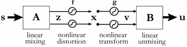
Figure 1: Building blocks of the PNL mixing model and the separating system.
2003). However, these methods—except the method of Harmeling et al. (2003)—are often compu-tationally very demanding and may face convergence problems in higher dimensions. In contrast, algorithms tailored to the PNL problem (Taleb and Jutten, 1999, Ziehe et al., 2001, Achard et al., 2001) are usually much simpler than those for the general problem, see Equation (1), since they only need to invert one-dimensional nonlinear functions, see Equation (2).
In this contribution, we propose a decoupled two-stage process to solve the PNL-BSS problem: first, we estimate the inverse functions gi of the component-wise non-linearities fi using the ACE algorithm (as described in Ziehe et al., 2001) or alternatively by applying a Gaussianizing transfor-mation (as in Ziehe et al., 2003a). After having equalized the nonlinearities, we can apply in the second step standard linear BSS techniques to recover the underlying source signals ( Figure 1).
Since the two stages—equalizing and unmixing—are independent from each other, the method can be easily generalized to handle also convolutive mixtures with PNL distortions, that is, mixed signals that are modeled as
x[t] = f
∑
τ A[τ]s[t−τ]
,
where A[τ]is an n×m filter matrix for eachτ. The sources s[t]can be simply recovered by replacing the BSS algorithm for instantaneous mixture with a method for convolutive unmixing (e.g. Parra and Spence, 2000, Murata et al., 2001).
The paper is organized as follows: in Subsection 2.1, we briefly introduce the ACE framework and prove that the algorithm converges to the correct inverse nonlinearities—provided that they exist. After that we propose an alternative linearization procedure employing Gaussianizing trans-formations in Subsection 2.2. In Section 3 we discuss some implementation issues and describe numerical simulations that illustrate our method. Finally, we give a conclusion in Section 4.
2. Methods
For the sake of simplicity, we introduce our method for the 2×2 case. The extension to the general case is briefly explained in the appendix. Let us consider the two-dimensional post-nonlinear mixing model:
x1= f1(A11s1+A12s2) x2= f2(A21s1+A22s2)
where s1and s2are independent source signals with time-structure, x1and x2 are the observed sig-nals, A= (Ai j)is the mixing matrix and f1and f2are the componentwise nonlinear transformations which are invertible.1
2.1 Maximizing Correlations with the ACE Algorithm
In order to invert the nonlinear functions f1and f2, we propose to maximize the correlation
corr(g1(x1),g2(x2)) (3)
with respect to some nonlinear functions g1and g2. That means, we want to find transformations g1 and g2of the observed signals such that the relationship between the transformed variables becomes linear. Intuitively speaking, the nonlinear transformation bends the data in a scatter plot away from a
straight line. Thus we have to find a transformation that nonlinearly squeezes and stretches the data in the scatter plot until the transformed signals have maximal correlation in order to undo the effect of the distortion (see Figure 4 for an illustration of this process). Under certain conditions that we will state in detail later, this problem is solved by the ACE method that finds so-called optimal transformations g∗1 and g∗2 which maximize Equation (3). Breiman and Friedman (1985) showed existence and uniqueness of those optimal transformations and proved that the ACE algorithm, which is described in the following, converges to these solutions (see Figure 4).
The ACE algorithm is an iterative procedure for finding the optimal nonlinear functions g∗1and g∗2. Starting from the observation that for fixed g1the optimal g2is given by
g2(x2) =E{g1(x1)|x2}, and conversely, for fixed g2the optimal g1is
g1(x1) =E{g2(x2)|x1},
we are ready to understand the key idea of the ACE algorithm that is to compute these conditional expectations alternately until convergence has been reached. To avoid trivial solutions g1(x1) is normalized in each step by using the function norm || · ||:= E{·}21/2
. The algorithm for two variables is summarized below. It is also possible to extend the procedure to the multivariate case, which is explained in Appendix A (for further details see Hastie and Tibshirani, 1990, Breiman and Friedman, 1985).
Algorithm 1 The ACE algorithm for two variables
{initialize}
g(0)1 (x1)← x1/||x1|| repeat
g(2k+1)(x2) ← E{g(1k) (x1)|x2}
˜
g(1k+1)(x1) ← E{g(2k+1)(x2)|x1}
g(1k+1)(x1) ← g˜(1k+1)(x1)/||g˜(1k+1)(x1)||
until E{g1(x1)−g2(x2)}2fails to decrease
The ACE algorithm was originally introduced to solve a special kind of regression problem, where one wants to find nonlinear transformations g1(·)and g2(·)such that g2(x2)explains g1(x1) optimally. The optimality is defined by the least squares criterion, that is,
min g1,g2
E{g1(x1)−g2(x2)}2
Eg21(x1) ,
where the denominator prevents scale indeterminacy. Interestingly, the optimal transformation in the least squares sense is equivalent to the transformation with maximal correlation,
max g1,g2
corr(g1(x1),g2(x2) ),
An important point in the implementation of the ACE algorithm is the estimation of the condi-tional expectations from the data. Usually, condicondi-tional expectations are computed by data smoothing for which numerous techniques exist (Breiman and Friedman, 1985, H ¨ardle, 1990). Our implemen-tation uses a nearest neighbor smoothing that applies a simple moving average filter to appropriately sorted data. Here the size of the moving average filter is a parameter to balance the trade-off between over- and under-smoothing.
In the following we want to verify that applying g∗1and g∗2 to the mixed signals x1 and x2, re-moves the effect of the nonlinear functions f1 and f2. To this end we show for z1=A11s1+A12s2 and z2=A21s1+A22s2that g∗1and g∗2obtained from the ACE procedure are the desired inverse func-tions given that z1and z2are jointly normally distributed, with other words we prove the following relationship:
h∗1(z1) := g1∗(f1(z1))∝z1 h∗2(z2) := g2∗(f2(z2))∝z2.
(4)
The proof proceeds exactly along the lines of Breiman and Friedman (1985). Noticing that the correlation of two signals does not change, if we scale one or both signals and following Proposition 5.4. and Theorem 5.3. of Breiman and Friedman (1985), we know that:
g∗1(x1)∝E{g∗2(x2)|x1} g∗2(x2)∝E{g∗1(x1)|x2}.
Here the conditional expectation E{g∗2(x2)|x1}is a function of x1and the expectation is taken with respect to x2, analogously for the second expression.
Since g∗1(x1) =h∗1(z1)and g∗2(x2) =h∗2(z2), furthermore x1= f1(z1)and x2= f2(z2)we get: h∗1(z1)∝E{h∗2(z2)|f1(z1)}
h∗2(z2)∝E{h∗1(z1)|f2(z2)}.
Because f1 and f2 are invertible functions they can be omitted in the condition of the conditional expectation, leading us to:
h∗1(z1)∝E{h∗2(z2)|z1} h∗2(z2)∝E{h∗1(z1)|z2}.
(5)
Assuming that the vector(z1,z2)>is normally distributed and the correlation coefficient corr(z1,z2)
is non-zero, a straightforward calculation shows
E{z2|z1}∝z1 E{z1|z2}∝z2.
This means that z1 and z2 satisfy Equation (5), which then immediately implies our claim Equa-tion (4).
It is favorable to our intended application that the above assumptions are usually fulfilled be-cause mixtures of independent signals have a distribution that is closer to a Gaussian according to the central limit theorem and that they are more correlated than unmixed signals. In practice, we see that the ACE algorithm is able to equalize the nonlinearities rather well, even if the assump-tions are not perfectly met, though there might be difficulties in the presence of strong noise or low correlations.
2.2 Transformations to Gaussian Random Variables
In the previous section we have argued that linearly mixed signals are most likely subject to Gaussian distributions due to the central limit theorem. This fact gives rise to a simple alternative for the ACE procedure in the first stage of our PNL-BSS method by making use of this Gaussianity assumption directly.
We propose to estimate the inverse functions of the true nonlinearities by finding transformations which convert each component into a Gaussian random variable (Gaussianization). Our Gaussian-ization technique is inspired by algorithms commonly used in random number surrogate generators and adaptive bin size methods (Pompe, 1993, Kantz and Schreiber, 1997). The goal is to find func-tions gi(·)such that
gi(xi)∼N(0,σ2i).
whereσ2i is set to a constant (e.g. σ2i =1) which can be done without loss of generality because scaling factors do not matter. The method, which is based on the ranks of samples and percentiles of the Gaussian distribution, proceeds as follows: suppose that the observed samples x[1], . . . ,x[T]
fulfill an ergodicity assumption and T is sufficiently large. Let r[t]be the rank of the t-th sample x[t]andΦ(·)be the cumulative distribution function of the standard Gaussian N(0,1). The ranks r are assumed to be ordered from the smallest value to the largest, e.g. r[t] =1 for t=argmintx[t]and r[t] =T for t=argmaxtx[t]. Then, the transformed samples
v[t] =Φ−1
r[t]
T+1
, t=1, . . . ,T
that is, the real values v[t]such thatΦ(v[t]) = Tr[+1t] can be regarded as realizations from the standard Gaussian distribution (c.f. Billingsley, 1995). Note that, adding 1 to the denominator is needed to avoid v=±∞. Furthermore, to limit the influence of outliers, we recommend to compute modified
versions of v[t]according to
v[t] =Φ−1
c r[t]
T+1+ (1−c) 1 2
, with 0<c<1.
The choice of c depends on the application, but is not critical. We used c=0.97 in our numerical experiments.
2.3 Source Separation
For a separation of the signals we could in principle apply any BSS technique that can solve linear problems. However, experiments show that second-order methods which use temporal information are more robust than higher-order based methods and allow to recover the sources more reliably in most natural applications.
Therefore we propose to use second-order BSS techniques that are based on the different time structure of the source signals. These methods (see Molgedey and Schuster, 1994, Belouchrani et al., 1997, Kawamoto et al., 1997, Pham and Garrat, 1997, Ziehe and M ¨uller, 1998, Yeredor, 2000) rely on the special structure of time-shifted covariance matrices of the mapped signals v[t] =g(x[t]). The key insight is that the pairwise cross-correlation functions of the components of the original signal s are zero for certain time lagsτ, that is,
Let u[t] =Bv[t]be an estimator of the original signal s[t]and
R(τ; B):= 1
2(T−τ)
T−τ
∑
t=1
n
u[t]u>[t+τ] +u[t+τ]u>[t]o,
be the symmetrized lagged covariance matrix of the estimator u, provided that u is already centered at 0. When we derive an estimator u close to the signal s, every lagged covariance matrix R(τ; B)
becomes approximately diagonal. Therefore, the task is to identify the demixing matrix B such that the covariance matrices R(0; B)and R(τk; B), k=1, . . . ,K are diagonal. This can be done by a joint diagonalization method, that is, to minimize the following criterion w.r.t. B under certain restrictions
L(B) =
∑
i6=j
R2i j(0; B) +
K
∑
k=1i
∑
6=jR2i j(τk; B),
where Ri j’s are the(i,j)-th components of the matrix R.
In the literature several methods to solve this constrained optimization problem exist (Cardoso and Souloumiac, 1996, Yeredor, 2000, Pham, 2001, Ziehe et al., 2003b). Here we use TDSEP, an im-plementation based on the efficient extended Jacobi method by Cardoso and Souloumiac (1996) for the simultaneous diagonalization of several time-delayed correlation matrices (Belouchrani et al., 1997, Ziehe and M ¨uller, 1998, M ¨uller et al., 1999).
3. Numerical Simulations
¿From now on we call the procedure based on ACE “ACE-TD” and analogously, the procedure based on Gaussianization “Gauss-TD”. To demonstrate the performance of the proposed approaches we apply these two methods to several post-nonlinear mixtures, both instantaneous and convolutive.
3.1 Toy Data: AR Processes
The first data set consists of Gaussian AR-processes of the form:
si[t] = M
∑
m=1
αmsi[t−m] +ξi[t], i=1, . . . ,n
whereξi[t]is white Gaussian noise with mean zero and varianceσ2. For the experiment we choose σ2=1, M=3, n=2 and generate 2000 data points. To the linearly mixed signals z we apply strong nonlinear distortions as in Taleb and Jutten (1999):
x1[t] = f1(z1[t]) =z31[t], (6)
x2[t] = f2(z2[t]) =tanh(10z2[t]).
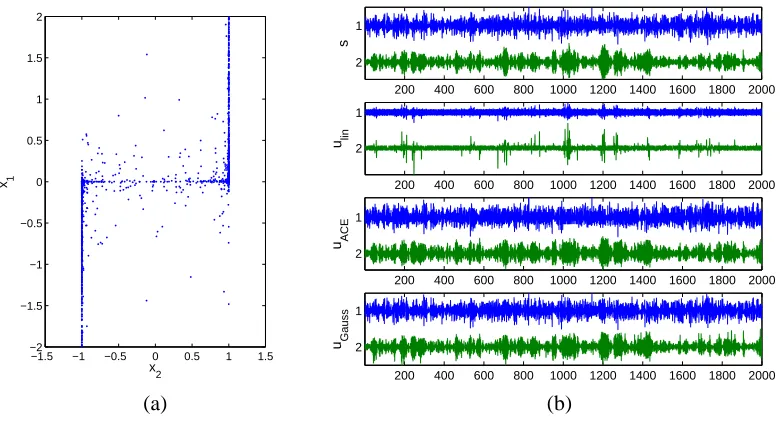
The distribution of these mixed signals has a highly nonlinear structure which is clearly visible in the scatter plot in Figure 2.
−1.5 −1 −0.5 0 0.5 1 1.5 −2 −1.5 −1 −0.5 0 0.5 1 1.5 2 x2 x1
200 400 600 800 1000 1200 1400 1600 1800 2000 2
1
s
200 400 600 800 1000 1200 1400 1600 1800 2000 2
1
u lin
200 400 600 800 1000 1200 1400 1600 1800 2000 2
1
u ACE
200 400 600 800 1000 1200 1400 1600 1800 2000 2
1
u Gauss
(a) (b)
Figure 2: (a) Scatter plot of the mixed AR-processes (x1[t]vs x2[t]) and (b) waveforms of the original sources
(first row), the linearly unmixed signals (second), recovered sources by ACE-TD (third) and those by Gauss-TD (fourth). The smoother for ACE has length 101. For Gauss-TDSEP we used time lagsτ=0. . .20.
−1 −0.5 0 0.5 1 −1 −0.5 0 0.5 1 f1
−1 −0.5 0 0.5 1 −1 −0.5 0 0.5 1 f2 (a)
−4 −2 0 2 4 −2 −1 0 1 2 g 1
−1.5 −1 −0.5 0 0.5 1 1.5 −1 −0.5 0 0.5 1 g 2 (b)
−4 −2 0 2 4 −2 −1 0 1 2 g 1
−1.5 −1 −0.5 0 0.5 1 1.5 −1 −0.5 0 0.5 1 g 2 (c)
Figure 3: (a) Nonlinear functions f1and f2. (b) True (thin line) and estimated (bold line) inverse functions g1and g2by the ACE method. (c) The same plots by the Gaussianizing transformation.
smoother (window length 101) has been used to compute the conditional expectation. We note that the remaining mismatch observed in Figure 3 (b) could be improved further by better smoothers.
iteration
0
scatter v histogram v1 histogram v2 g1 g2
2
30
Figure 4: Monitoring of the iterative ACE procedure. The rows correspond to snapshots of the iteration at initialization and after two resp. thirty steps. The columns show a scatter plot of transformed data v (first column), histograms of v1(second) and v2(third), estimated inverse functions g1(fourth) and g2(fifth).
−3 −2 −1 0 1 2 3
−4 −3 −2 −1 0 1 2 3 4
−3 −2 −1 0 1 2 3
−4 −3 −2 −1 0 1 2 3 4
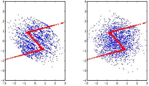
Figure 5: Left panel: scatter plot of the output distribution of a linear (’+’) and the proposed nonlinear ACE-TD algorithm (’.’). Right panel: similar plot with the nonlinear Gauss-TD algorithm (’.’).
Figure 2 (b) shows that the waveforms of the recovered sources by ACE-TD (the third row) and by Gauss-TD (the fourth row) closely resemble the original ones, while the result of the linear unmixing of the PNL mixture (the second row) can not recover the sources as is expected. This is also confirmed by comparing the output distributions that are shown in Figure 5. The left panel shows the scatter plots of the distributions obtained by TDSEP and ACE-TD, respectively. In the right panel we show the corresponding scatter plots for TDSEP and Gauss-TD, which indeed looks much more Gaussian.
3.2 Instantaneously Mixed Speech Data
The source signals are linearly mixed by a 4×4 random matrix A, i.e. z[t] =As[t]. After the linear mixing the following nonlinearities were applied:
f1(z1) = 0.1z1+0.1z31 f2(z2) = 0.3z2+tanh(3z2) f3(z3) = tanh(2z3)
f4(z4) = z34.
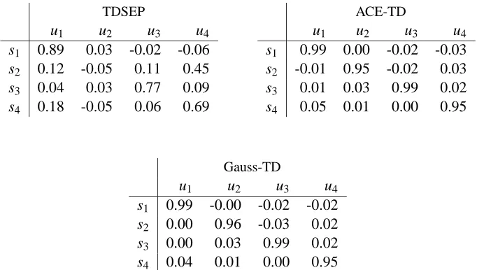
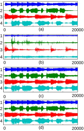
In order to apply the ACE-TD method to this dataset, we have to employ the multivariate version of the ACE algorithm which is explained in Appendix A. As in the two-variables case, the extended version of ACE guarantees the identifiability of the inverses g1(·), . . . ,gn(·) under the Gaussianity assumption, although there is an asymmetry in the treatment of these functions (for details see Ap-pendix A). On the other hand, the extension of Gauss-TD to the multivariate case is straightforward. Figure 6 shows the results of the separation using ACE-TD (with smoothing window length 101 and time delaysτ=0. . .30) and Gauss-TD (with time delaysτ=0. . .30) in the panels (c) and (d). We observe again very good separation performances that are quantified by calculating the cor-relation coefficients between the source signals and the extracted components (see Table 1). This is also confirmed by listening to the separated audio signals, where we perceive almost no crosstalk, although the noise level is slightly increased (c.f. the silent parts of signal 2 in Figure 6 (a), (c) and (d)).
TDSEP
u1 u2 u3 u4
s1 0.89 0.03 -0.02 -0.06 s2 0.12 -0.05 0.11 0.45
s3 0.04 0.03 0.77 0.09
s4 0.18 -0.05 0.06 0.69
ACE-TD
u1 u2 u3 u4
s1 0.99 0.00 -0.02 -0.03 s2 -0.01 0.95 -0.02 0.03
s3 0.01 0.03 0.99 0.02
s4 0.05 0.01 0.00 0.95
Gauss-TD
u1 u2 u3 u4
s1 0.99 -0.00 -0.02 -0.02 s2 0.00 0.96 -0.03 0.02
s3 0.00 0.03 0.99 0.02
s4 0.04 0.01 0.00 0.95
Table 1: Correlation coefficients for the signals shown in Figure 6 .
20000
4
3
2
1
(a)
0
20000
4
3
2
1
(b)
0
20000
4
3
2
1
(c)
0
20000
4
3
2
1
(d)
0
Figure 6: Four channel audio dataset: (a) waveforms of the original sources, (b) linearly unmixed sig-nals with TDSEP, (c) recovered sources using ACE-TD and (d) recovered sources using Gauss-TD. A smoother with window length 101 was used in ACE and time lags τ=0. . .30 were employed for the separation. The audio files corresponding to these experiments are also available on the web page
algorithms statistics s1 s2 s3 s4
TDSEP median 0.7285 0.6341 0.6710 0.6448
#{corr>0.9} 3 1 1 1
ACE-TD median 0.9585 0.9480 0.9527 0.9533
(window length 101) #{corr>0.9} 77 66 73 75
ACE-TD median 0.9084 0.8918 0.8946 0.9125
(window length 17) #{corr>0.9} 56 45 45 57
Gauss-TD median 0.9831 0.9800 0.9790 0.9748
#{corr>0.9} 94 93 89 86
Table 2: Maximum correlation between sources and recovered signals. ’median’ denotes the median of the 100 trials and ’#{corr>0.9}’ is the number of trials which gave correlations larger than 0.9. In ACE, besides the smoother with window length 101, we also used a shorter window length (=17), which however resulted in under-smoothed nonlinearity estimators. In the separation with TDSEP time lagsτ=0. . .30 have been used.
window length (H¨ardle, 1990); however, the detailed analysis of this issue exceeds the scope of this contribution.
3.3 Speech Data: Convolutive Mixtures
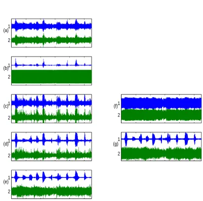
The third experiment gives an example of applying our method to convolutive mixtures with a PNL distortion. With nonlinear transfer functions as in our first example (c.f. Equation (6)), we delib-erately distorted real-room recordings2 of speech and background music (from Lee et al., 1998). For the separation we apply a convolutive BSS algorithm of Parra and Spence (2000) that requires only second-order statistics and exploits the non-stationarity of the signals. While an unmixing of the distorted recordings obviously fails, we could achieve a good separation after the unsupervised linearization by the ACE procedure or the Gaussianization (c.f. Figure 7).
3.4 Comparison to Taleb and Jutten (1999)
The standard method for PNL-BSS (due to Taleb and Jutten, 1999), abbr. TJ, estimates simultane-ously the linear and the nonlinear part of the mixing model. This is done by minimizing a contrast function based on mutual information. For this the densities have to be estimated which is a difficult problem on its own. In contrast, Gauss-TD decouples the linear and the nonlinear stages and solves each one separately by simple methods (Gaussianization and TDSEP).
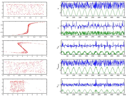
To keep the computational efforts for TJ within a reasonable range, we use a dataset with two channels and 500 samples for the simulation. The sources are random uniform noise and a sinusoidal signal as shown in the upper panel of Figure 9. The sources were mixed with a 2×2 mixing matrix and componentwise distorted using the nonlinear transfer functions:
x1[t] = f1(z1[t]) =z31[t],
x2[t] = f2(z2[t]) =tanh(2z2[t]).
2 1 (a)
2 1 (b)
2 1 (c)
2 1 (d)
2 1 (e)
2 1 (f)
2 1 (g)
Figure 7: Two channel audio dataset: (a) waveforms of the recorded (undistorted) microphone signals, (b) observed PNL distorted signals, (c) result of ACE (smoothing window length 101), (d) recovered sources using ACE and a convolutive BSS algorithm and (e) for comparison convolutive BSS separation result for undistorted signals from (a). The right panels: (f) result of Gaussianizing transformation and (g) recovered sources using Gaussianization and a convolutive BSS algorithm. For listening to these audio data we refer to
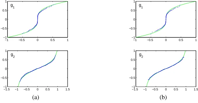
This data is shown in the second row of Figure 9. A linear separation of these signals obviously fails as can be seen in the third row of Figure 9. Only after the non-linear distortions have been equalized by the estimated inverse functions (shown in Figure 8), blind separation is successful and yields signals that closely resemble the underlying sources. The last row of Figure 9 shows the results of Taleb and Jutten’s method. We observe a good separation except for a few points at the edges of the scatter plot. These problems are possibly due to the fixed bin size in the kernel density estimators used by this method. This emphasizes again the need for better smoothers and adaptive bin size methods. However, since Gauss-TD results are comparable (c.f. 4th and 5th row of Figure 9), Gauss-TD is often due to its simplicity the method of choice.
−1 −0.5 0 0.5 1
−1 −0.5 0 0.5 1
g
1
−1.5 −1 −0.5 0 0.5 1 1.5 −1
−0.5 0 0.5 1
g
2
(a)
−1 −0.5 0 0.5 1
−1 −0.5 0 0.5 1
g
1
−1.5 −1 −0.5 0 0.5 1 1.5 −1
−0.5 0 0.5 1
g
2
(b)
Figure 8: (a) True (thin line) and estimated (bold line) inverse functions g1and g2obtained by the
Gaussian-ization method. (b) The same plots for the Taleb-Jutten (TJ) algorithm.
4. Discussion and Conclusion
In this work we proposed a simple technique for blind separation of linear mixtures with post-nonlinear distortions based on ACE resp. Gaussianization with a subsequent application of BSS: ACE-TD and Gauss-TD. The algorithms proceed in two steps: first, ACE-TD searches nonlinear transformations that maximize the linear correlations between the transformed variables. Hereby it approximates the inverses of the nonlinearities. This search can be done efficiently by applying the ACE technique (Breiman and Friedman, 1985) from non-parametric statistics that performs an alternating estimation of conditional expectations by the smoothing of scatter plots. The bottom line is that the nonlinear re-transformation reduces the PNL mixing problem to a linear one. This allows us to apply a linear BSS algorithm as a second step. While in principle any ICA/BSS method could be used, second-order techniques (e.g. Belouchrani et al., 1997, Ziehe and M ¨uller, 1998) are more consistent with the Gaussianity assumptions, because in higher-order ICA methods the source signals are required to be non-Gaussian. Second-order methods are less influenced by remaining, small non-linear distortions.
−2 −1.5 −1 −0.5 0 0.5 1 1.5 2 −2 −1 0 1 2
−0.8 −0.6 −0.4 −0.2 0 0.2 0.4 0.6 −1
−0.5 0 0.5 1
−4 −3 −2 −1 0 1 2 3 4 5
−2 −1 0 1 2
−2 −1.5 −1 −0.5 0 0.5 1 1.5 2 −2
−1 0 1 2
−3 −2 −1 0 1 2 3 4 5 6
−2 −1 0 1 2
50 100 150 200 250 300 350 400 450 500 2
1
s
50 100 150 200 250 300 350 400 450 500 2
1
x
50 100 150 200 250 300 350 400 450 500 2
1
ulin
50 100 150 200 250 300 350 400 450 500 2
1
uGauss
50 100 150 200 250 300 350 400 450 500 2
1
uTJ
Figure 9: Scatter plots and waveforms for the sources, mixed and unmixed signals (c.f. Figure 1). From top to bottom row we see true source signals, observed post-nonlinear mixtures, linearly unmixed signals, separation results of Gauss-TD, separation results of Taleb and Jutten’s algorithm.
1985, H¨ardle, 1990). Furthermore, Gauss-TD is a computationally simpler alternative of ACE-TD, since the former estimates the inverses of the nonlinearities directly by Gaussianizing the individual components. Gaussianization was also employed as an initialization of a more sophisticated PNL algorithm and turned out to improve computational speed substantially (Sol ´e et al., 2003). Both al-gorithms have theoretical guarantees to yield the correct results, if the linearly mixed signals before the PNL distortion are Gaussian distributed and provided that there is none or only low additive noise present after the post-nonlinearity. Because of the central limit theorem, the Gaussianity as-sumption usually holds approximately in practice, especially if the number of sources are large and the mixing matrix is not sparse. While the Gaussianization gives satisfactory results under these as-sumptions, the ACE method may run into difficulties if the correlations of the linearly mixed signals are low (see also the discussion in Breiman and Friedman, 1985).
In contrast to methods that simultaneously estimate the mixing matrix, the nonlinear equaliza-tion funcequaliza-tions and the distribuequaliza-tions of sources (like e.g. Taleb and Jutten, 1999, Achard et al., 2001, S. Achard and Jutten, 2003), our two-stage procedures are computational more attractive. They work well with large data sets and scale linearly with respect to the number of sources. Interest-ingly, our methods can be easily applied to convolutive mixtures, which is important for solving the real-room “cocktail-party” problem with BSS (see also Koutras, 2002). Here occasionally nonlinear transfer functions of the sensors (microphones) or the use of class C amplifiers can hinder a proper separation.
Concluding, the proposed framework gives simple algorithms of high efficiency with a solid theoretical background for signal separation in applications with a PNL distortion that are of im-portance, for example, in real-world sensor technology. In our simulations the simpler Gauss-TD algorithm compares favorably to ACE-TD and to mutual information based methods as proposed by Taleb and Jutten (1999). However, it is conceivable that further improvements of the smoothing pro-cedure will lead to increased performance of the ACE and other methods relying on non-parametric density estimation. Future research will therefore be concerned with incorporating domain knowl-edge for a better tuning of the smoothers to improve and robustify the separation performance.
Acknowledgements
This work is the extended version of Ziehe et al. (2001, 2003a). This work has been partially supported by the European Community under the Information Society Technology (IST) RTD pro-gramme, contract IST-1999-14190-BLISS. The authors are solely responsible for the content of this article. It does not represent the opinion of the European Community, and the European Community is not responsible for any use that might be made of data appearing therein.
Appendix A. The Multi-dimensional ACE Algorithm
Whenever there are more than two sensors, we apply the multivariate ACE algorithm (Breiman and Friedman, 1985, Hastie and Tibshirani, 1990, H¨ardle, 1990):
Algorithm 2 The ACE algorithm for multi-dimensional cases
{initialize}
g(0)1 (x1)← x1/||x1||and g(0)2 (x2), . . . ,g(0)n (x2) =0 repeat
for i=2 to n do: g(ik+1)(xi) ← E{g(
k)
1 (x1)−∑j<ig (k+1)
j (xj)−∑j>ig (k)
j (xj)|xi} end for loop
g1(k+1)(x1) ← E{∑nj=2g(jk+1)(xj)|x1}/kE{∑nj=2g (k+1)
j (xj)|x1}k until E{g1(x1)−∑nj=2gj(xj)}2fails to decrease
This general ACE algorithm yields transformations g1(·), . . . ,gn(·) which minimize the least squares error
min g1,...,gn
E{g1(x1)−∑nj=2gj(xj)}2 Eg2
1(x1)
As in the case of two variables, it has been proven in Breiman and Friedman (1985) that the opti-mal transformations in the least squares sense are equivalent to the transformations with maxiopti-mal correlation,
max g1,...,gn
corr(g1(x1),
n
∑
j=2
gj(xj) ),
up to scaling factors.
Hence, if the linearly mixed signals z are jointly Gaussian distributed, we can recover the inverse functions g1(·), . . . ,gn(·)of the true nonlinearities with the multi-dimensional ACE algorithm. For details we refer to the proof presented in Breiman and Friedman (1985).
As a final remark, we note that in the original ACE algorithm one component—e.g. x1—is treated somewhat special as the “response” variable, while the BSS problem is intrinsically sym-metric with respect to the components x1, . . . ,xn. Therefore, the development of a symmetric version of this algorithm is left as a topic for further research.
References
S. Achard, D.-T. Pham, and C. Jutten. Blind source separation in post nonlinear mixtures. In T.-W. Lee, editor, Proc. Int. Workshop on Independent Component Analysis and Blind Signal Separation (ICA2001), pages 295–300, San Diego, California, 2001.
S. Amari, A. Cichocki, and H.-H. Yang. A new learning algorithm for blind source separation. In D. S. Touretzky, M. C. Mozer, and M. E. Hasselmo, editors, Advances in Neural Information Processing Systems, volume 8, pages 757–763. MIT Press, Cambridge, MA, 1996.
A.J. Bell and T.J. Sejnowski. An information-maximization approach to blind separation and blind deconvolution. Neural Computation, 7:1129–1159, 1995.
A. Belouchrani, K. Abed Meraim, J.-F. Cardoso, and E. Moulines. A blind source separation tech-nique based on second order statistics. IEEE Trans. on Signal Processing, 45(2):434–444, 1997.
P. Billingsley. Probability and Measure. John Wiley & Sons, New York, 1995.
L. Breiman and J.H. Friedman. Estimating optimal transformations for multiple regression and correlation. Journal of the American Statistical Association, 80(391):580–598, 1985.
J.-F. Cardoso and A. Souloumiac. Blind beamforming for non Gaussian signals. IEE Proceedings-F, 140(6):362–370, 1993.
J.-F. Cardoso and A. Souloumiac. Jacobi angles for simultaneous diagonalization. SIAM J.Mat.Anal.Appl., 17(1):161–164, 1996.
P. Comon. Independent component analysis—a new concept? Signal Processing, 36:287–314, 1994.
G. Deco and D. Obradovic. Linear redundancy reduction learning. Neural Networks, 8(5):751–755, 1995.
S. Harmeling, A. Ziehe, M. Kawanabe, and K.-R. M ¨uller. Kernel feature spaces and nonlinear blind source separation. In T.G. Dietterich, S. Becker, and Z. Ghahramani, editors, Advances in Neural Information Processing Systems, volume 14, pages 761–768. MIT Press, 2002.
S. Harmeling, A. Ziehe, M. Kawanabe, and K.-R. M ¨uller. Kernel-based nonlinear blind source separation. Neural Computation, 15:1089–1124, 2003.
T.J. Hastie and R.J. Tibshirani. Generalized Additive Models, volume 43 of Monographs on Statis-tics and Applied Probability. Chapman & Hall, London, 1990.
A. Hyv¨arinen, J. Karhunen, and E. Oja. Independent Component Analysis. Wiley, 2001.
A. Hyv¨arinen and E. Oja. A fast fixed-point algorithm for independent component analysis. Neural Computation, 9(7):1483–1492, 1997.
C. Jutten and J. H´erault. Blind separation of sources, part I: An adaptive algorithm based on neu-romimetic architecture. Signal Processing, 24:1–10, 1991.
C. Jutten and J. Karhunen. Advances in nonlinear blind source separation. In Proc. of the 4th Int. Symp. on Independent Component Analysis and Blind Signal Separation (ICA2003), pages 245–256, Nara, Japan, April 1-4 2003. Invited paper in the special session on nonlinear ICA and BSS.
H. Kantz and T. Schreiber. Nonlinear time series analysis. Cambridge University Press, Cambridge, UK, 1997.
M. Kawamoto, K. Matsuoka, and M. Oya. Blind separation of sources using temporal correlation of the observed signals. IEICE Trans. Fundamentals, E80-A(4):695–704, 1997.
A. Koutras. Blind separation of nonlinear convolved speech mixtures. In Proc. ICASSP 2002, pages 913–919, Orlando, Florida, 2002.
L. E. Larson. Radio frequency integrated circuit technology low-power wireless communications. IEEE Personal Communications, 5(3):11–19, 1998.
T.-W. Lee, B.U. Koehler, and R. Orglmeister. Blind source separation of nonlinear mixing models. IEEE International Workshop on Neural Networks for Signal Processing, pages 406–415, 1997.
T.-W. Lee, A. Ziehe, R.Orglmeister, and T.J. Sejnowski. Combining time-delayed decorrelation and ICA: Towards solving the cocktail party problem. In Proc. ICASSP98, volume 2, pages 1249–1252, Seattle, 1998.
J. K. Lin, D. G. Grier, and J. D. Cowan. Faithful representation of separable distributions. Neural Computation, 9(6):1305–1320, 1997.
G. Marques and Luis B. Almeida. Separation of nonlinear mixtures using pattern repulsion. In Proc. Int. Workshop on Independent Component Analysis and Signal Separation (ICA’99), pages 277–282, Aussois, France, 1999.
K.-R. M¨uller, S. Mika, G. R¨atsch, K. Tsuda, and B. Sch ¨olkopf. An introduction to kernel-based learning algorithms. IEEE Transactions on Neural Networks, 12(2):181–201, 2001.
K.-R. M¨uller, P. Philips, and A. Ziehe. JADET D: Combining higher-order statistics and temporal information for blind source separation (with noise). In Proc. Int. Workshop on Independent Component Analysis and Signal Separation (ICA’99), pages 87–92, Aussois, France, 1999.
N. Murata, S. Ikeda, and A. Ziehe. An approach to blind source separation based on temporal structure of speech signals. Neurocomputing, 41(1-4):1–24, 2001.
P. Pajunen, A. Hyv¨arinen, and J. Karhunen. Nonlinear blind source separation by self-organizing maps. In Proc. Int. Conf. on Neural Information Processing, pages 1207–1210, Hong Kong, 1996.
P. Pajunen and J. Karhunen. A maximum likelihood approach to nonlinear blind source separation. In Proceedings of the 1997 Int. Conf. on Artificial Neural Networks (ICANN’97), pages 541–546, Lausanne, Switzerland, 1997.
P. Pajunen and J. Karhunen, editors. Proc. of the 2nd Int. Workshop on Independent Component Analysis and Blind Signal Separation (ICA200). Otamedia, Helsinki, Finland, 2000.
L.C. Parra and C. Spence. Convolutive blind source separation of non-stationary sources. IEEE Trans. on Speech and Audio Processing, 8(3):320–327, 2000. US Patent US6167417.
D.-T. Pham. Joint approximate diagonalization of positive definite matrices. SIAM J. on Matrix Anal. and Appl., 22(4):1136–1152, 2001.
D.-T. Pham and P. Garrat. Blind separation of mixture of independent sources through a quasi-maximum likelihood approach. IEEE Trans. on Signal Processing, 45(7):1712–1725, 1997.
B. Pompe. Measuring statistical dependences in a time series. J. Stat. Phys., 73:587–610, 1993.
D.-T. Pham S. Achard and C. Jutten. Quadratic dependence measure for nonlinear blind sources separation. In Proc. 4th Intern. Symp. on Independent Component Analysis and Blind Signal Separation (ICA2003), pages 263–268, Nara, Japan, 2003.
B. Sch¨olkopf and A.J. Smola. Learning with Kernels. MIT Press, Cambridge, MA, 2002.
B. Sch¨olkopf, A.J. Smola, and K.-R. M ¨uller. Nonlinear component analysis as a kernel Eigenvalue problem. Neural Computation, 10:1299–1319, 1998.
J. Sol´e, M. Babaie-Zadeh, C. Jutten, and D.-T. Pham. Improving algorithm speed in PNL mixture separation and Wiener system inversion. In Proc. Int. Conf. on Independent Component Analysis and Signal Separation (ICA2003), Nara, Japan, April 2003.
A. Taleb. A generic framework for blind source separation in structured nonlinear models. IEEE Trans. on Signal Processing, 50(8):1819–1830, 2002.
A. Taleb and C. Jutten. Source separation in post-nonlinear mixtures. IEEE Trans. on Signal Processing, 47(10):2807–2820, 1999.
H. Valpola, X. Giannakopoulos, A. Honkela, and J. Karhunen. Nonlinear independent component analysis using ensemble learning: Experiments and discussion. In Proc. Int. Workshop on Inde-pendent Component Analysis and Blind Signal Separation (ICA2000), pages 351–356, Helsinki, Finland, 2000.
H. Valpola, E. Oja, A. Ilin, A. Honkela, and J. Karhunen. Nonlinear blind source separation by variational Bayesian learning. IEICE Transactions (Japan), E86-A(3), March 2003. To appear in a Special Section on Blind Signal Processing (Invited paper).
V. N. Vapnik. Statistical Learning Theory. Wiley, New York, 1998.
H.-H. Yang, S. Amari, and A. Cichocki. Information-theoretic approach to blind separation of sources in non-linear mixture. Signal Processing, 64(3):291–300, 1998.
A. Yeredor. Blind separation of gaussian sources via second-order statistics with asymptotically optimal weighting. IEEE Signal Processing Letters, 7(7):197–200, 2000.
A. Ziehe, M. Kawanabe, S. Harmeling, and K.-R. M ¨uller. Separation of post-nonlinear mixtures using ACE and temporal decorrelation. In T.-W. Lee, editor, Proc. Int. Workshop on Indepen-dent Component Analysis and Blind Signal Separation (ICA2001), pages 433–438, San Diego, California, 2001.
A. Ziehe, M. Kawanabe, S. Harmeling, and K.-R. M ¨uller. Blind separation of post-nonlinear mixtures using gaussianizing transformations and temporal decorrelation. In Proc. 4th In-tern. Symp. on Independent Component Analysis and Blind Signal Separation (ICA2003), pages 269–274, Nara, Japan, April 2003a.
A. Ziehe, P. Laskov, K.-R. M ¨uller, and G. Nolte. A linear least-squares algorithm for joint diag-onalization. In Proc. 4th Intern. Symp. on Independent Component Analysis and Blind Signal Separation (ICA2003), pages 469–474, Nara, Japan, 2003b.
A. Ziehe and K.-R. M ¨uller. TDSEP–an efficient algorithm for blind separation using time structure. In Proc. Int. Conf. on Artificial Neural Networks (ICANN’98), pages 675–680, Sk ¨ovde, Sweden, 1998.