Efficient SVM Training Using Low-Rank Kernel
Representations
Shai Fine [email protected]
Human Language Technologies Department IBM T. J. Watson Research Center
P.O. Box 218, Yorktown Heights, NY 10598, USA
Katya Scheinberg [email protected]
Mathematical Science Department IBM T. J. Watson Research Center
P.O. Box 218, Yorktown Heights, NY 10598, USA
Editors:Nello Cristianini, John Shawe-Taylor and Bob Williamson
Abstract
SVM training is a convex optimization problem which scales with the training set size rather than the feature space dimension. While this is usually considered to be a desired quality, in large scale problems it may cause training to be impractical. The common techniques to handle this difficulty basically build a solution by solving a sequence of small scale subproblems. Our current effort is concentrated on the rank of the kernel matrix as a source for further enhancement of the training procedure. We first show that for a low rank kernel matrix it is possible to design a better interior point method (IPM) in terms of storage requirements as well as computational complexity. We then suggest an efficient use of a known factorization technique to approximate a given kernel matrix by a low rank matrix, which in turn will be used to feed the optimizer. Finally, we derive an upper bound on the change in the objective function value based on the approximation error and the number of active constraints (support vectors). This bound is general in the sense that it holds regardless of the approximation method.
Keywords: Support Vector Machine, Interior Point Method, Cholesky Product Form, Cholesky Factorization, Approximate Solution
1. Introduction
(Platt, 1999), which sequentially update one or two (resp.) Lagrange multipliers at every training step, and active set methods, such as Chunking (Boser et al., 1992), Decomposition (Osuna et al., 1997) and Shrinking (Joachims, 1999), which gradually build the (hopefully) small set of active constraints by feeding a generic optimizer (usually an interior point algorithm) with small scale subproblems.
Our current effort is concentrated on the numerical rank of the kernel matrix as a source for further enhancement of the performance of the IPM. To this end we make the following three key observations:
1. If the kernel matrix has low rank, then it is possible to design an efficient interior point method that scaleslinearlywith the size of data set.
2. If the kernel matrix has full rank (or almost so), it may be possible to approximate it by a low rank positive semidefinite matrix (which in turn can be used to feed the optimizer).
3. By using an approximation matrix instead of the original kernel matrix we obtain a perturbed optimization problem, which requires less computational effort to solve. In general, the optimal value of the objective function of the perturbed problem is different than the optimal value of the original problem. However, the size of the difference can be explicitely controlled by the quality of the approximation.
We assume that the positive semidefinite kernel matrix, Qn×n, is totally dense and too
large to handle, however its rank,k, is significantly smaller than n(“significantly” may be defined according to the context). This means that Q can be represented as Q = V VT, whereV is a matrix withkcolumns andnrows. The most expensive step at every iteration of an IPM (applied to an SVM problem) is inverting or factorizing a matrix of the form
D+Q, where D is a diagonal (positive) matrix and Q is as described above. In general, this operation requires O(n2) storage space and takesO(n3) arithmetic operations, but by handling the linear algebra in a special way we can reduce the complexity to O(nk2) and the storage to O(nk).
There are two possible approaches that achieve the same complexity. The first approach is based on the Sherman-Morrison-Woodbury formula for a low rank update of an inverse of a matrix. The Sherman-Morrison-Woodbury formula has been used widely in the context of interior point methods for linear programming (Choi et al., 1990, Marxen, 1989). In that context, however, the method often runs into numerical difficulties. The second approach is based on product form Cholesky factorization and is described in Section 3. This method is somewhat more expensive than the first: its workload is about twice and the storage requirement is three times the storage needed for the first method. On the other hand, the second method was shown to be numerically stable (experimentally and theoretically) in the context of interior point methods for LP and quadratically constrained quadratic problems (Goldfarb and Scheinberg, 1999). Some examples that we present in Section 3 suggest that the first method may also have numerical difficulties in the context of our QP problems. The second method works well numerically for all problems that we tried.
of Q is close to (or equal to) n, Q can be approximated by a low rank symmetric posi-tive semidefinite matrix ˜Q. In this case one can apply incomplete Cholesky factorization method with symmetric pivoting to obtain the desired representation ofQor its approxima-tion. This procedure requiresO(nk2) operations, where kis the number of nonzero pivots in the procedure, which is the same as the rank of matrixQ or of its low rank approxima-tion. The storage requirements reduces to O(nk). It is possible to trace the quality of the approximation and apply an appropriate stopping criteria without an extra effort. This and the overall complexity makes this method compare favorably with other recently suggested approximation techniques (Smola and Sch¨olkopf, 2000, Williams and Seeger, 2001).
Finally, the last observation leads us to derive a bound on the quality of the solution obtained by solving the perturbed problem using a low rank approximation toQ. We show that if the approximation errorQ−Q˜ is bounded (in some sense) by, then the difference between the optimal objective function values of the original problem and the perturbed problems is bounded bylc2, where c is the penalty (cost) parameter of the training error
and lis the number of active points in the training set of the perturbed problem.
The rest of this paper is organized as follows: In the next section we present the convex QP that we are interested in solving, and the interior point method that we use. In Section 3 we describe the Sherman-Morrison-Woodbury method and the product form Cholesky factorization method, as means for low rank updates. Section 4 is devoted to issues related to approximating the kernel matrix by a low-rank positive semidefinite matrix. We present the algorithm to find such an approximation and a theorem in which we derive the above mentioned bound. Experiments, which demonstrate the utility of the suggested method, are presented in Section 5. We wrap things up in Section 6 with some concluding remarks and leading directions for further study.
1.1 Notation
In general we denote scalars and vectors in lower case letters (we make an explicit distinction when it is not clear from the context), and we use upper case letters to denote matrices. We use subscript indices to indicate elements of a vector or a matrix and we use superscript to label a whole matrix of a vector with an index.
The description in this paper follows the traditional notation used in the optimization literature, which is slightly different from the one used in most SVM papers. The main difference is in the identification of the primal and dual problems (which switch roles) and the convention used to denote the unknowns with x, y, while in the SVM literature x and
y are used to denote the input vectors and their labels, resp. Hence, the SVM training problem with 1-norm soft margin is
minξ,w,b
1
2w, w+c
n
i=1 ξi
(SV M) s.t. ai(w, vi+b)≥1−ξi, i= 1, . . . , n
ξi≥0, i= 1, . . . , n
shorthand for the labeled kernel matrix, i.e.
Qi,j =aiajK(vi, vj)
whereK(·,·) is a (Mercer) kernel function representing dot-products in the feature (RKHS) space.
We will use an equivalent form of the above problem (with somewhat different notation) which we will refer to as the dual problem (see problem (D) in the next section). The dual of the (SV M) problem is thus called theprimalproblem (see problem (P) in the next section).
2. An Interior Point Method
We consider the following convex quadratic programming problem.
minx
1 2x
T
Qx−eTx
(P) s.t. aTx= 0,
0≤x≤c,
where x∈Rn is the vector of primal variables, e is the vector of all 1’s of lengthn and a
is a vector of labels, 1’s and −1’s. c is the penalty parameter associated with the training error. In general it may be desirable to use different penalty parameters for different data points. In this case c should be treated as an n-dimensional vector. However, for the sake of simplicity we assume thatcis a positive scalar. All our analysis and results extend easily to the more general case. Similarly, one might want to solve a problem with a slightly more general objective function 12xTQx+qTx, whereqis somen-dimensional vector (e.g., a small scaled optimization problem arising within a chunking-like meta algorithms). Our analysis and results extend easily to this case as well.
The dual to the above problem is
maxy,s −
1 2x
T
Qx−c n
i=1 ξi
(D) s.t. −Qx+ay+s−ξ=−e,
s≥0, ξ≥0,
Here y is the scalar dual variable (it is equal to the negative bias) and s and ξ are the
n-dimensional vectors of dual variables.
Both (P) and (D) have finite optimal solutions and any optimal primal-dual pair of solutions satisfies the Karush-Kuhn-Tucker (KKT) necessary and sufficient optimality con-ditions:
Xs= 0,
aTx= 0,
−Qx+ay+s−ξ =−e,
0≤x≤c, s≥0, ξ≥0.
By X (S, C−X) we denote the diagonal matrix whose diagonal entries are the elements of the vectorx (s,c−x). For optimality conditions of QP and details of applying IPMs to QP (see Wright, 1997) and references therein.
The perturbed KKT optimality conditions
Xs=σµe,
(C−X)ξ =σµe
(CPµ) a
T x= 0,
−Qx+ay+s−ξ=−e,
0≤x≤c, s≥0, ξ≥0
have a unique solution for any positive values of the parameter µ and σ. The trajectory of solutions to the above system of equations for all values of µ ∈ (0,∞) with some fixed positive value of σ is called the central path. The central path converges to an optimal solution. A path-following primal-dual interior point method tries to follow the central path towards the optimal solution by iteratively approximating solutions on the path by applying the Newton method to the above system of nonlinear equations, while reducing the value of parameterµ on each iteration.
Any typical interior point method solves a linearization of the above system of nonlinear equations. We use the so-called Mehrotra predictor-corrector algorithm (Mehrotra, 1992), which is considered to be one of the most efficient in practice, however the ideas presented in Section 3 on reducing the per-iteration complexity apply to any other interior point method. At every iteration there are two basic steps - the predictor step and the corrector step. The idea behind this algorithm is to start with “predicting” the best reduction in the duality gap, by evaluating a step directly towards the optimality. Such step, however, is not taken, since it may ruin the “centrality” of the iterates. A corrector step is computed instead. The corrector step enforces the centrality and also takes into account the approximate curvature of the central path predicted by the predictor step.
Predictor step is a Newton step towards the solution of the system with σ = 0 (which is the same as the system of the KKT conditions). Then, using this step, a value for σ is chosen and a better step (corrector step) towards solution of the above system with this value of σ is taken.
For the predictor step we compute (∆x,∆y,∆s,∆ξ), satisfying
−Q a I −I
aT 0 0 0
S 0 X 0
−Ξ 0 0 (C−X)
∆x ∆y ∆s ∆ξ = rc rb −Xs
−(C−X)ξ
where rb = −a T
x, rc = −e+Qx−ay−s+ξ. If the current solution is primal and dual
By eliminating ∆s, ∆ξ and consequently ∆x from the system we obtain an expression for ∆y: aT(Q+D)−1a∆y = r, where D = SX−1+ Ξ(C −X)−1 and r is a right hand side that depends on (Q+D)−1 and other parameters of the system. Solving for ∆y we substitute it back to find ∆x, ∆sand ∆ξ. The maximum possible step length is determined by computing α≤1 such that 0≤x+α∆x≤c, 0≤s+α∆sand 0≤ξ+α∆ξ.
To compute the corrector step, we set dx = ∆x, ds = ∆s and dξ = ∆ξ and ˆµ = (x +dx)T(s+ds) + (c−x−dx)T(ξ +dξ) (from the predictor step) and compute new (∆x,∆y,∆s,∆ξ), satisfying
−Q a I −I
aT 0 0 0
S 0 X 0
−Ξ 0 0 (C−X)
∆x ∆y ∆s ∆ξ = rc rb
σµ−dXds−Xs σµ+dXdξ−(C−X)ξ
whereσ is defined by
σ = ˆ µ µ 3 .
We solve this system similarly to the system for the predictor step, compute the largest possible step (but actually take 99% of that step to avoid hitting the boundaries of the feasible region or else the new solution would not be in the interior), and update the current solution.
The stopping criteria is formed by checking the duality gap and the primal and dual feasibility against a predetermined tolerance. If these conditions are still not met, we compute a new value for the parameterµand repeat the iteration. This algorithm converges to an optimal solutions from any strictly interior starting point (a point that lies inside all inequality constraints). In theory, it takes O(nln(1/)) iterations to converge, where is the relative accuracy. However, in practice, an interior point method rarely takes more than 50 iterations, regardless of the problem’s size.
The most time consuming operation on every step is obtaining a vector of the form
u= (Q+D)−1w (e.g., during the computation of the predictor step such operation is done twice - once during computation of the right hand side vectorrand once during computation of aT(Q+D)−1a). Since Q+Dis a dense n×n, symmetric positive definite matrix, then
in general obtaining the vectoru requiresO(n3) operations. Typically this can be done by either computing the inverse or factorizing1 Q+D.
The main point of the next section is to show that ifQcan be represented asQ=V VT, whereV isn×kmatrix (wherek << n), then vectorucan be obtained inO(k2n) operations. 3. Low-rank updates
There are two methods which efficiently solve the system (D+V VT)u=w by taking into consideration the special form of the matrix of the system (i.e., the fact that it is a diagonal matrix plus a low-rank symmetric positive semidefinite matrix). Both of these methods requireO(nk) storage andO(nk2) arithmetic operations, wherekis the number of columns
inV. Thus, ifk << nthen the two methods provide significant savings in terms of workload and storage.
The first method is somewhat cheaper than the second. Its workload is about half of that of the second method and the storage requirement is one third of the storage of the second method. On the other hand, the first method may experience numerical instability.
3.1 Sherman-Morrison-Woodbury update
We consider a classical method for a low-rank update of an inverse of a matrix. This update is usually called the Sherman-Morrison-Woodbury (SMW) update or formula:
(D+V VT)−1=D−1−D−1V(I+VTD−1V)−1VTD−1.
Since we would like to avoid storing the matrix D+V VT, we also would like to avoid storing its inverse. We can apply the above formula to solve the system (D+V VT)u=w
as follows:
u=D−1w−D−1V(I+VTD−1V)−1VTD−1w.
Hence, compute
z:=D−1w
t: (I +VTD−1V)t=VTz u:=z−D−1V t.
The system in the second step is k×k symmetric positive definite and can be solved by computing Cholesky factorization of (I +VTD−1V). The work required to compute such factorization is O(k3), which is small if k is small with respect to n. Computing the matrix of that system takes nk2/2 +O(nk) multiplications (and the same number of additions). The overall work, in terms of the number of multiplications, required to solve (D+V VT)u=wis nk2/2 plus smaller order terms.
The Sherman-Morrison-Woodbury has been used widely in the context of interior point methods for linear programming, (Choi et al., 1990, Marxen, 1989). In that context, how-ever, the method often runs into numerical difficulties. There are few modifications of the method that have been proposed to deal with the numerical instability (Andersen, 1996, Scheinberg and Wright, 2000). However, these modifications do not always help, and they increase the computational cost.
It is not easy to point out rigorously the situations for which the SMW formula is numerically unstable. The intuition suggests that it happens when matrixD+V VT or just
Dis not well conditioned. Consider the following small example:
Example 1 Let
D=
2
1
and V =
1
−1
.
D+V VT ≈
1 −1
−1 2
. (1)
Now consider solving (D+V VT)u = w, where w =
w1
w2 and w1 and w2 are Θ(1).
Clearly
u≈
2w1+w2 w1+w2 .
(2)
Let us apply the Sherman-Morrison-Woodbury formula to this example.
z=
w1
2 w2
(VTD−1V +I)t= (2 + 1
2)t and V T
z= w1
2 −w2.
Because of round-off errors VTD−1V +I is computed as 1/2 and VTz as w1/2. Hence t=w1,
u=z−D−1V t=
w1
2 − w1
2 w2+w1 =
0
w2+w1 .
Clearly, the computed solution is not even close to the approximately correct solution (2).
A tuation similar to the above example happens often in linear programming. For our QP problems such a situation is less natural, but still possible. The diagonal elements ofDare
si/xi+ξi/(c−xi). By complementarity, asµapproaches zero, eithersi →0 andxi →x∗i >0
or xi → 0 and si → s∗i > 0 (analogously, either ξi → 0 and xi → x∗i < c or xi → c and ξi →ξi∗>0). Moreover, whenever a variable converges to zero, it converges with the same
rate as the parameter µ. Thus, whenever si and ξi both converge to zero (which happens
for the points that are in the active optimal set), then Di converges to zero with the same
rate asµ. Otherwise,Di converges to infinity with the same rate as 1/µ. Ifµ= 10−8, then
some elements ofDare of the order 10−8 and the others are of the order 108. If we scaleD
andQby 10−8 thenDlooks similar to the diagonal matrix in the example; i.e., some of the
elements are of the order of 1 and some are of the order of 10−16(which often is the order of the machine precisions). To have matrixQandV consistent with the example, we need the elements of scaled matrix 10−8Qto be of the order of 1. This will happen if the elements of V, e.g. the data points, are of the order 104. In section 5 we briefly discuss some examples of practical SVM problems for which our implementation of the interior point method with the SMW update failed to converge.
In the next subsection we present an alternative method, which avoids many of the numerical difficulties of the SMW update.
3.2 Product-Form Cholesky Factorization
Here a Cholesky factorization of a symmetric positive semidefinite matrixM ∈Rn×n is defined asM =LΛLT, whereLis a lower triangular matrix with ones on the diagonal, and Λ is a nonnegative diagonal matrix. A product form Cholesky factorization, in general, is of the form ˜L1L˜2. . .L˜kΛ˜k( ˜Lk)T. . .( ˜L2)T( ˜L1)T, where each ˜Li is a lower triangular matrix and ˜Λk is a nonnegative diagonal matrix.
To solve a system of linear equations M u=w, one has to solve the following sequence of linear systems: ˜L1u1 =w, ˜L2u2 =u1,. . . , ˜Lkuk = uk−1, ( ˜Lk)Tuk+1 = (Λk)−1uk, . . . , ( ˜L1)Tu =u2k−1. Each such system has a lower triangular or an upper triangular matrix, and, in a general dense case, solving each such system takesO(n2) operations. However, if
each ˜Li has a special structure (such as we will see below) then solving each system takes only O(n) operations.
Let us assume that we have a Cholesky factorization of a matrix M: M =LΛLT. We would like to obtain a product form factorization of M +vvT, where v ∈ Rn is a vector (hence,vvT is a rank-one n×nmatrix):
LΛLT +vvT =L(Λ +ppT)LT =LL˜Λ ˜˜LTLT,
wherep is the solution of the equationsLp =v and ˜LΛ ˜˜LT is the Cholesky factorization of Λ +ppT.
˜
L has a special form
˜
L=
1
p2β1 1
p3β1 p3β2 1
..
. ... ... . ..
pn−1β1 pn−1β2 pn−2β3 · · · 1 pnβ1 pnβ2 pnβ3 · · · pnβn−1 1
, (3)
where β ∈ Rn and ˜Λ = diag{λ˜1, . . . ,λ˜n} can be computed from the following recurrence
relations:
t0 := 1,
forj= 1,2, . . . , n
tj :=tj−1+p2j/λj,
˜
λj :=λjtj/tj−1, βj :=pj/(λjtj).
Various versions of this method for updating Cholesky factorization by a rank-one term were proposed by Bennet (1965), Fletcher and Powell (1974) and Gill et al. (1975).
If we allow someλjto be zero, then it is easy to verify that the above recurrence relations
become:
It is often important for the purpose of numerical stability to consider λj as equal to
t0:= 1,
forj= 1,2, . . . , n
if tj−1 =∞
if λj = 0
tj :=tj−1+p2j/λj,
˜
λj :=λjtj/tj−1, βj :=pj/(λjtj).
else
if pj = 0
tj :=∞
˜
λj :=p2j/tj−1, βj := 1/pj.
else
tj :=tj−1
˜
λj := 0 βj := 0
else
tj :=∞
˜
λj :=λj, βj := 0.
Figure 1: Rank-One update for Product-Form Cholesky Factorization
Now assume that we have a factorization LΛLT and we want to obtain a product form factorization ofLΛLT+v1(v1)T+v2(v2)T+. . .+vk(vk)T. By repeating the above procedure
k times, once for each rank-one term vi(vi)T, we can obtain the product from Cholesky factorizationLL˜1L˜2. . . ,L˜kΛ˜k( ˜Lk)T. . .( ˜L2)T( ˜L1)TLT from the following:
Procedure 1.
1. Set ˜Λ0 := Λ, 2. Fori= 1, . . . , k
(i) Solve Lq0,i=vi forq0,i;
(ii) For j= 1, . . . , i−1, solve ˜Ljqj,i=qj−1,i forqj,i;
In the case of our QP problems, we need to compute product form Cholesky factorization of a matrixM =D+V VT, whereDis a diagonal matrix inRn×n,V is a rectangular matrix in Rn×k (assuming k << n), and V VT =ki=1vi(vi)T, where vi is thei-th column ofV. Thus, we can apply the above Procedure 1 by setting initial Λ to equal Dand L toIn, an n×nidentity matrix.
To store information about the product form Cholesky factorization of (D+V VT) we need to store the matrix V, the diagonal elements of Λk, k vectors pi and k vectors βi,
i= 1, . . . k. Overall, our memory requirement for the factorization is 3knplus smaller order terms.
To compute the vectorspi andβi,i= 1, . . . , k, we need to solve (k−1)(k−2)/2 systems of the form ˜Lq =r (by ˜L, without an index, we mean any matrix of the form of Eq. (3)). Due to the special structure of ˜Lsuch solution can be obtained by the following procedure:
Procedure 2. Given p,β andr;
1. Setq:=r andσ :=q1β1;
2. Forj= 2, . . . , n
Setqj :=qj−pjσ,
σ :=σ+qjβj
This procedure requires 2nmultiplications (and the same number of additions). Recur-sions in Fig. 1 requireO(n) operations for eachi= 1, . . . , k. Hence, overall, the computation of the product from Cholesky factorization of D+V VT requires k2n ( plus smaller order term) multiplications.
Clearly, solving the system of equations of the form ˜LTq = r, and performing matrix multiplicationq = ˜Lrorq= ˜LTreach can be done by a procedure which takes into account the special structure of ˜L, similarly to Procedure 2, and requires O(n) operations. Thus, once the factorization of D+V VT is computed, solving (D+V VT)u = w requires only
O(kn) operations. The overall complexity in terms of the number of multiplications is then
k2nplus smaller order term. This is about twice as much as the complexity of solving this system using the SMW update. However, ifk << nthis complexity is still a very significant improvement overO(n3) operations required to solve (D+V VT)u=w directly.
the case of linear programming. The proof of numerical stability does not apply directly, and extending it is tedious and beyond interest of this paper; however, similar intuition applies. Computational experiments show that the product form Cholesky factorization method avoids numerical difficulties even when the initial data is not well conditioned.
4. Approximating the Kernel Matrix
It is often the case that the exact low-rank representation of the kernel matrix Q=V VT
is not given, or even does not exist, i.e. the rank of Q is large. In these cases we may hope that Q can at least be approximated2 by a low rank matrix ˜Q. However, finding a good approximation while keeping its rank low is not trivial. In this section we address the following problem: given a symmetric positive semidefinite matrix, Q, construct a matrix
˜
Qsuch that its rankk and the bound on the error ∆Q=Q−Q˜ are acceptably small. Recently, Smola and Sch¨olkopf (2000) suggested a method for approximating the data set in the feature space by a set in a low-dimensional subspace. The authors suggested to select (via random sampling) a small subset of data points to form the basis of the approximating subspace3 . All other data points are then approximated by linear combinations of the elements of the basis. The basis is build iteratively, each new candidate element is chosen by a greedy method to reduce the bound on the approximation error ∆Q=Q−Q˜ as much as possible. The authors use the value tr(∆Q) as the bound on the norm of ∆Q, and hence, as a stopping criteria: the algorithm stops when tr(∆Q) is below some tolerance, say tol.
Let us assume that k points are already in the basis. To compute the reduction of the approximation bound for each of the remainingn−kpoints extraO(nk(n−k)) operations are required. This is clearly too expensive. The authors suggest at each iteration to randomly selectN candidates for the basis and apply their greedy approach only to those candidates. Thus, the overall complexity isO(N nk2).
Here we present a way of constructing ˜Qby directly approximating the Cholesky factor-ization ofQ. The proposed algorithm has complexity O(nk2) and takes the full advantage of the greedy approach for the best reduction in the approximation bound tr(∆Q).
Any positive definite matrix Q can be represented by its Cholesky factorization Q =
GGT, where G is a lower triangular matrix4 (see Golub and Van Loan, 1996, Ch. 4). If
Qis positive semidefinite and singular, then it is still possible to compute an “incomplete” Cholesky factorization GGT, where some columns of Gare zero. Such procedure requires
O(k2n) operations, where k is the number of nonzero pivots in the procedure, which is the same as the rank of matrix Q. This procedure can also be applied to almost singular matrices by skipping pivots that are below a certain threshold (see Golub and Van Loan, 1996). If the eigenvalues ofQare distinctly separated into a group of very small eigenvalues and relatively large eigenvalues then by choosing an appropriate value of the threshold such procedure will produce both: very small numerical error and a good approximation
2. Indeed in the context of SVMit was already been noted that typicallyQhas rapidly decaying eigen-values (Williamson et al., 1998, Smola and Sch¨olkopf, 2000) although there exist kernels for which their eigenspectrum is flat (Oliver et al., 2000).
3. Also see Williams and Seeger (2001) for another random sampling technique for low rank approximation. 4. This is the traditional definition of Cholesky factorization. It relates to the definition presented at Section
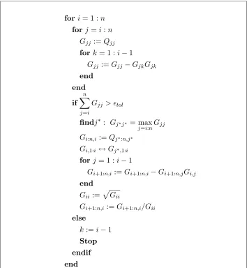
(see Wright, 1996). If, however, the eigenvalues of Q have a more complicated structure (varying from very small to relatively large), then a symmetric permutation of rows and columns ofQmay be necessary during the Cholesky factorization procedure to stabilize the computations and guarantee a good approximation. Symmetric permutations (sometimes referred to as “symmetric pivoting”, cf. 4.2.9 of Golub and Van Loan 1996) are also crucial in case when one is trying to find the best possible approximation while keeping the rank of the approximating matrix below a prescribed bound. Figure 2 present an algorithm which computes an approximation ˜Q=GGT of Qusing incomplete Cholesky factorization with symmetric permutations. Note that this procedure generates theCholesky triangle G
column by column, while keeping in memory only the diagonal elements of Q. All other entries ofQare needed only once and thus can be computed on demand. Hence it is easy to derive a “kernelized” version of the suggested procedure, assuming an access to the input vectors and the kernel function.
fori= 1 :n
for j=i:n
Gjj:=Qjj
fork= 1 :i−1
Gjj :=Gjj−GjkGjk
end
end
if
n
j=i
Gjj > tol
findj∗: Gj∗j∗ = max j=i:nGjj Gi:n,i:=Qj∗:n,j∗
Gi,1:i ↔Gj∗,1:i
forj= 1 :i−1
Gi+1:n,i:=Gi+1:n,i−Gi+1:n,jGi,j
end
Gii:=
Gii
Gi+1:n,i:=Gi+1:n,i/Gii
else
k:=i−1 Stop
endif
end
The computational complexity of this procedure is O(nk2), since the only extra work is in computing diagonal elementsGjj, which requiresO(nk) operations at each iteration. The
storage requirement isO(nk). Symmetric permutations provide a greedy way of building the approximation ofQ. After i iterations of the Cholesky factorization procedure the matrix
Gi =G1:n,1:i is such that Gi(Gi) T
= ˜Qi, where ˜Qi is an approximation of Q subject to a symmetric permutation of rows and columns. For simplicity, let us assume that the rows and columns ofQare ordered “correctly” and no permutation is necessary (this assumption does not affect our analysis). Let ∆Qi =Q−Q˜i. LetGi1:i be the matrix composed of the
first irows ofGi and Gii+1:nin the matrix composed of the last n−icolumns. Then
∆Qi =
0 0
0 Qi+1:n,i+1:n−Gii+1:n(Gi1:i)−1Q1:i,i+1:n
.
From the properties of Cholesky factorization, ∆Qi is positive semidefinite and it is easy to see that after updatingGjj for allj=i+ 1, . . . , nat thei-th iteration,nj=iGjj = tr ∆Qi.
Thus, when the above algorithm stops (afterkiteration), we have tr ∆Q≤tol.
4.1 Bound on the error in the optimal objective value
Consider the perturbed optimization problem ( ˜P), which is constructed by replacing the kernel matrixQ by a low-rank approximation ˜Q, i.e.
minx
1 2x
T ˜
Qx−eTx
( ˜P) s.t. aTx= 0,
0≤x≤c.
A natural question to ask is: How close is the solution of the perturbed problem to the solution of the original problem.
Let x∗ denote an optimal solution of the original problem (P) and let ˜x∗ denote an optimal solution of the perturbed problem ( ˜P). Also let f denote the objective function of (P), and ˜f be the objective function of ˜P. We would like to estimate|f(x∗)−f˜(˜x∗)|. The feasible sets of P and ˜P are the same, hence a feasible solution of one problem is feasible for the other.
From optimality of ˜x∗ f˜(˜x∗) ≤ f˜(x∗) = f(x∗) + 12(x∗)T∆Qx∗. We know that ∆Q =
Q−Q˜ is positive semidefinite, thus ˜f(˜x∗) ≤f˜(x∗)≤f(x∗); i.e. optimal objective value of the perturbed problem is always smaller than the optimal objective value of the original problem5.
On the other hand, optimality of x∗ f(x∗) ≤ f(˜x∗), hence f(x∗)−f˜(˜x∗) ≤ f(˜x∗)− ˜
f(˜x∗) = 12(˜x∗)T∆Qx˜∗ ≤ 12λ1(∆Q)||x˜∗||2 ≤ 12tr (Q−Q˜)||x˜∗||2. Let l be the number of
positive components of ˜x∗. From the feasibility constraints 0≤x≤cthese components are bounded from above by c. Let ∆Ql be the principal sub-matrix of ∆Qthat corresponds to
positive components of ˜x∗. The above yields the bound
0≤f(x∗)−f˜(˜x∗)≤ 1 2x(0)
T
∆Qx(0)≤ c
2l
2 .
Hence we have the following theorem:
Theorem 1 If (Q−Q˜)is positive semidefinite andtr (Q−Q˜)≤then the optimal objective value of the original problem is larger than the optimal objective value of the perturbed problem and their difference is bounded byc2l/2, wherelis the number of active constraints (support vectors) in the perturbed problem.
The above error bound does not require approximation matrix ˜Q to be obtained by Cholesky factorization with permutations. Theorem 1 holds for any ˜Q such that Q−Q˜ is positive semidefinite and it’s trace is bounded by . If Q−Q˜ is not positive semidefinite, then it is still possible to provide a bound on the change in the optimal value function through a bound on the norm of ∆Q(see Fine and Scheinberg 2001 for more details).
5. Experiments
In this section we compare performances of the suggested method to state-of-the-art SVM training procedures, construct a simple toy example to demonstrate the numerical instabil-ity of the Sherman-Morrison-Woodbury update, and examined the impact of approximating the SVM solution from both the optimization problem and the classification problem per-spectives.
5.1 Cholesky Product Form QP vs. SMO
We’ve modeled 150 different Speaker Id binary problems6, in the following way: For each speaker we trained a mixture of 4 Gaussians, 25 dimensions7, diagonal covariance. We then applied Fisher kernel methodology (Jaakkola and Haussler, 1999), which resulted in transforming the original data vectors to a 204 dimensional space. We further applied linear normalization transformation to each dimension to balance the transformed vectors. This caused the transformed vectors to be fully dense. The size of the training set in a typical problem ranges from 6500 to 7000 vectors, roughly equally divided to positive and negative example. We chose a dot-product kernel and compared our technique with the SMO algorithm to find a maximal margin linear separator. Our choice was motivated by former evidences which support the claim that most of the work in separating the positive and negative points is carried out through the transformation represented by the Fisher kernel. In the current setting the choice of a dotproduct kernel served another purpose -to obtain results of the SMO at the peek of its performance. To this end we used a special designed variant of SMO which takes advantage of the fact that the kernel operations are just dot-products (for further discussion see Platt, 1999). The comparison in CPU time (depicted at Fig. 3) clearly favors our method. Note also that we have gained roughly a
6. This is part of a much larger multi-class Speaker ID system (Fine, Navr´atil, and Gopinath, 2001). 7. 13 dimension cepstrum, augmented with first derivatives (‘delta’) and finally discarding the energy
0 50 100 150 102
103 104 105
SpeakerID using Fisher Kernel
Binary Problems
CPU: log(sec)
DotProduct SMO Cholesky Product Form QP
Figure 3: Cholesky Product Form QP vs. SMO
factor of 1100 in computational complexity and a factor of 33 in the storage requirements over traditional IPMs.
5.2 Cholesky Product Form QP vs. SVMlight
1 2 3 4 5 6 7 8 9 10 100
101 102 103 104
SVMlight vs. CholQP on Abalone data set (4177 x 10)
Chunk size (x10)
CPU: log(sec)
Svmlight C=0.2 Svmlight C=1 Svmlight C=10 CholQP C=0.2,1,10
Figure 4: Cholesky Product Form QP vs. SVMlight
problem, while our method (denoted “CholQP” it the figure) is stable for all levels of difficulty.
5.3 Example of failure of the Sherman-Morrison-Woodbury update
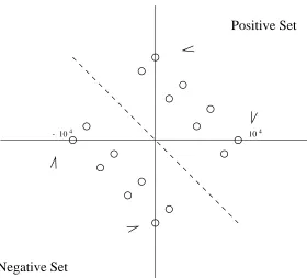
We constructed a small example in the spirit of the one described in Section 3 to demon-strate possible numerical instability of the Sherman-Morrison-Woodbury update. Figure 5 illustrates the data in the example. There are two crucial features: the set of active support vectors is redundant (so the problem is degenerate) and the support vectors are scaled by a large number (104). On this problem an interior point method using SMW update failed to converge after achieving only 2 digits of accuracy. The same IPM with the product form Cholesky update converged to 8 digits of accuracy.
To demonstrate that such failures can happen in practice we applied the Sherman-Morrison-Woodbury version of the code to an approximate problem arising from Abalone data set using polynomial kernel (as described in the next subsection). The algorithm stalled after achieving only 5 digits of accuracy, whereas the product form Cholesky version converged to 12 digits of accuracy.
5.4 Incomplete Cholesky Factorization (ICF)
4
Negative Set
Positive Set
104
- 10
Figure 5: Example for the failure of SMW update
at (Smola and Sch¨olkopf, 2000) on the Abalone data set8 using polynomial kernels, i.e.
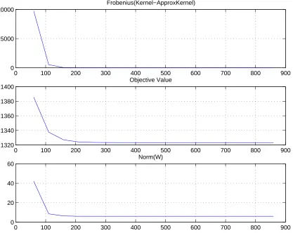
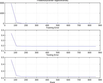
k(x, y) = (x, y+const)d. Thus we actually used the “kernelized” version of the factor-ization algorithm (cf. Section 4). We examined the resulted factorfactor-ization from two stand points: Figure 6 demonstrates the impact of the low-rank approximation on the solution of the optimization problem as a function of the rank, i.e. the optimal value of the objec-tive function9 and the norm of the separating hyperplane. Figure 7 shows the impact of the low-rank approximation from the classification performances perspective, i.e. training and testing errors. Both figures are scaled with a graph which measures the quality of the approximation in Frobenius norm (the square root of the sum of squares of the matrix elements) with respect to the original kernel matrix.
6. Concluding Remarks
Our experiments show that an IPM (with the proposed approach to linear algebra) can be more efficient than other state-of-the-art methods for QP problems arising in the course of training support vector machines, if the kernel matrix has a low rank (compared to the size of the data) or if it can be approximated by a low-rank positive semidefinite matrix. We considered two possible ways of handling linear algebra. We showed that Sherman-Morrison-Woodbury update may be numerically unstable. However, if accuracy is not a
8. The data set was preprocessed as described in Section 5.2, and we used the first 3000 points for training and the remaining 1177 points for testing.
0 100 200 300 400 500 600 700 800 900 0
5000 10000
Frobenius(Kernel−ApproxKernel)
0 100 200 300 400 500 600 700 800 900
1320 1340 1360 1380 1400
Objective Value
0 100 200 300 400 500 600 700 800 900
0 20 40 60
Norm(W)
Figure 6: Incomplete Cholesky Factorization for Poly Kernel (input dim = 10, poly degree = 5) on the Abalone data set. The optimization problem perspective: optimal value of the objective function and norm of the separating hyperplane. X axis is the rank (note that the feature space dim≈3000).
high priority one might prefer to use the SMW method over the product form Cholesky factorization, since it is faster and requires less storage.
For massive data sets which do not fit the memory restrictions, an IPM may still be the most efficient approach to solve smaller subproblems. This motivates an effort to em-bed our approximation technique and QP solver in a Chunking/Shrinking meta algorithm. Such a scheme is expected to enhance performance in terms of storage requirement and computational complexity and, thus, it will enable to efficiently handle larger chunks.
0 100 200 300 400 500 600 700 800 900 0
5000 10000
Frobenius(Kernel−ApproxKernel)
0 100 200 300 400 500 600 700 800 900
0.1 0.2 0.3 0.4 0.5
Training Error
0 100 200 300 400 500 600 700 800 900
0.2 0.3 0.4 0.5
Testing Error
Rank
Figure 7: Incomplete Cholesky Factorization for Poly Kernel (input dim = 10, poly degree = 5) on the Abalone data set. The classification problem perspective: training and testing errors. X axis is the rank (note that the feature space dim≈3000).
Working out a bound for the approximation error that will ensure the identification of the active set is a subject for future research.
Acknowledgments
The authors wishes to thank Ramesh Gopinath for pointing out a shorter proof of Theorem 1, and to the anonymous referees for their useful comments and suggestions.
References
J. M. Bennet. Triangular factors of modified matrices.Numerisches Mathematik, 7:217–221, 1965.
C. L. Blake and C. J Merz. UCI repository of machine learning databases, 1998. URL
http://www.ics.uci.edu/∼mlearn/MLRepository.html.
B. Boser, I. Guyon, and V. N. Vapnik. A training algorithm for optimal margin classifiers. In D. Haussler, editor,Proceedings of the 5th Annual ACM Workshop on Computational Learning Theory, pages 144–152. ACM Press, 1992.
I. C. Choi, C. L. Monma, and D. F. Shanno. Further development of primal-dual interior point methods. ORSA J. on Computing, 2(4):304–311, 1990.
S. Fine, J. Navr´atil, and R. A. Gopinath. A hubrid gmm/svm approach to speaker iden-tification. In Proc. of the International Conference on Acoustics, Speech, and Signal Processing (ICASSP), 2001.
S. Fine and K. Scheinberg. Efficient application of interior point methods for quadratic problems arising in support vector machines using low-rank kernel representation. Sub-mitted to Mathematical Programming, 2001.
R. Fletcher and M. J. D. Powell. On the modification ofldlT factorization. Mathematics of Computation, 28(128):1067–1087, 1974.
T. T. Friess, N. Cristianini, and C. Campbell. The kernel-adaraton algorithm: A fast simple learning procedure for support vector machines. InProceedings of the 15th International Conference on Machine Learning, pages 188–196. Morgan Kaufman, 1998.
Ph. E. Gill, W. Murray, and M. A. Saunders. Methods for computing and modifying the ldv factors of a matrix. Mathematics of Computation, 29:1051–10, 1975.
D. Goldfarb and K. Scheinberg. A product-form cholesky factorization method for handling dense columns in interior point methods for linear programming. Submitted, 1999.
G. H. Golub and Ch. F. Van Loan. Matrix Computations. The Johns Hopkins University Press, Baltimore and London, 3 edition, 1996.
T. S. Jaakkola and D. Haussler. Exploiting generative models in discriminative classifiers. In M. S. Kearns, S. A. Solla, and D. A. Cohn, editors, Advances in Neural Information Processing Systems, volume 11. MIT Press, 1999.
T. Joachims. Making large-scale support vector machine learning practical. In B. Sch¨olkopf, C. C. Burges, and A. J. Smola, editors, Advances in Kernel Methods, chapter 12, pages 169–184. MIT Press, 1999.
A. Marxen. Primal barrier methods for linear programming. Technical report, Dept. of Operations Research, Stanford University, Stanford, CA, 1989.
N. Oliver, B. Sch¨olkopf, and A. J. Smola. Natural regularization from generative models. In A. J. Smola, B. Sch¨olkopf, P. L. Bartlett, and D. Schuurmans, editors, Advances in Large Margin Classifiers, chapter 4, pages 51–60. MIT Press, 2000.
E. Osuna, R. Freund, and F. Girosi. An improved training algorithm for support vector ma-chines. InProceedings of the IEEE Neural Networks for signal Processing VII Workshop, pages 276–285. IEEE, 1997.
J. C. Platt. Fast trining support vector machines using sequential mininal optimization. In B. Sch¨olkopf, C. C. Burges, and A. J. Smola, editors, Advances in Kernel Methods, chapter 12, pages 185–208. MIT Press, 1999.
K. Scheinberg and S. Wright. A note on modified cholesky and schur complement in interior point methods for linear programming. Manuscript, 2000.
A. J. Smola and B. Sch¨olkopf. Sparse greedy matrix approximation for machine learning. In Proceedings of the 17th International Conference on Machine Learning, pages 911–918, Stanford University, CA, 2000. Morgan Kaufmann Publishers.
V. N. Vapnik. The Nature of Statistical Learning Theory. Springer-Verlag, 1995.
C. Williams and M. Seeger. Using the nystr¨om method to speed up kernel machines. In Todd K. Leen, Thomas G. Dietterich, and Volker Tresp, editors, Advances in Neural Information Processing Systems 13, pages 682–688. MIT Press, 2001.
R. C. Williamson, A. J. Smola, and B. Sch¨olkopf. Generalization performance of regulariza-tion networks and support vector machines via entropy numbers of compact operators. NeuroCOLT NC-TR-98-019, Royal Holloway College, University of London, UK, 1998.
S. Wright. Modified cholesky factorizations in interior point algorithms for linear program-ming. Preprint anl/mcs-p600-0596, Argonne National Laboratory, Argonne, IL, 1996.