Jointly Informative Feature Selection Made Tractable by Gaussian Modeling

(1)

Jointly Informative Feature Selection Made Tractable by

Gaussian Modeling

Leonidas Lefakis∗ [email protected]

Zalando Research Zalando SE Berlin, Germany

Fran¸cois Fleuret [email protected]

Computer Vision and Learning group Idiap Research Institute

Martigny, Switzerland

Editor:Amos Storkey

Abstract

We address the problem of selecting groups of jointly informative, continuous, features in the context of classification and propose several novel criteria for performing this selection. The proposed class of methods is based on combining a Gaussian modeling of the feature responses with derived bounds on and approximations to their mutual information with the class label. Furthermore, specific algorithmic implementations of these criteria are presented which reduce the computational complexity of the proposed feature selection algorithms by up to two-orders of magnitude. Consequently we show that feature selection based on the joint mutual information of features and class label is in fact tractable; this runs contrary to prior works that largely depend on marginal quantities. An empirical evaluation using several types of classifiers on multiple data sets show that this class of methods outperforms state-of-the-art baselines, both in terms of speed and classification accuracy.

Keywords: feature selection, mutual information, entropy, mixture of Gaussians

1. Introduction

Given a collection of data in RD it is often advantageous to reduce its dimensionality by either extracting (Hinton and Salakhutdinov, 2006) or selecting (Guyon and Elisseeff, 2003) a subset ofdDfeatures, which carry “as much information as possible”. The motivation behind this dimensionality reduction can be either to control over-fitting by reducing the capacity of the classifier space or to improve the computational overhead by reducing the optimization domain. It can also be used as a tool to facilitate the understanding or the graphical representation of high-dimensional data.

In the present work we focus on the selection, rather than extraction, of features. In general feature selection methods can be divided into two large families: Techniques from the first group,filters, are predictor agnostic as they do not optimize the selection of features

(2)

for a specific prediction method. They are usually based on classical statistics or informa-tion theoretic tools; the novel methods we propose in this article belong to this category. Techniques from the second group, wrappers, choose features to optimize the performance of a certain predictor. They usually require the retraining of the predictor at each step of a greedy search. Consequently they are typically computationally more expensive than filters. Furthermore, as the selected features are tailored to a specific predictor, they often do not work well with other families of predictors.

In the following we present a filter approach to feature selection in the context of classi-fication based on the maximization of the mutual information between the selected features and the class to predict. The use of mutual information as a criterion for feature selec-tion has been extensively studied in the literature, and can be motivated in the context of classification by Fano’s inequality

H(Y|Yˆ)≤1 +P(e) log (|Y|-1)

whereY,Yˆ are the true and predicted labels respectively, whileeis the event thatY 6= ˆY. Combining the above with the data processing inequality (specifically the chain Y →X →

ˆ

Y) results in the following lower bound on the probability of an incorrect classification PE

by

P(e)≥ H(Y)−I(X;Y)−1

(|Y|-1)

whereH(Y) is the entropy of the class prior andI(X;Y) is the mutual information between the output (Y) and input (X) features.

An important issue that arises in this context, is that of the joint “informativeness” of the selected features. Though wrappers by their very nature tend to select features which are jointly informative, this issue is only partially addressed for filters due to the resulting computational complexity and need for very large training sets. Most existing methods (Peng et al., 2005; Fleuret, 2004; Hall and Smith, 1999; Liu and Yu, 2003) typically compromise by relying on the mutual information between individual features or very small groups of features (pairs, triplets) and the class. We argue however, that rather than compromising on the joint behavior of the selected features, it is preferable to accept a compromise on the density model, which will allow to analyze this joint behavior in an efficient manner.

In a classification task with continuous features context, if we aim at taking into account the joint behavior of features, a Gaussian model is a natural choice. This unfortunately leads to a technical difficulty: If such a model is used for the conditional distributions of the features given the class then the non-conditioned distribution is a mixture of Gaussians and its entropy has no simple analytical form. There is extensive prior work on the problem of approximating the entropy of a mixture of Gaussians (Hershey and Olsen, 2007), but most of the existing approximations are too computationally intensive to be used during an iterative optimization process which requires the estimation of the mutual information of a very large number of subsets of features with the class to predict.

(3)

on updating the inverses of covariance matrices iteratively instead of computing them from scratch drastically reducing the computational cost during the optimization of the selected feature set.

2. Related Works

When selecting d features from a pool of D candidates in the context of a classification task, it does not suffice to select features independently informative with respect to the class. When such greedy strategies are employed the risk of acquiring redundant, or even identical, features increases. Thus, it is also important that these features exhibit low redundancy between them: joint informativeness is at the core of feature selection.

As mentioned in the introduction, wrappers, due to their very nature, address this issue by creating subsets of features that perform well when combined with a specific predictor. Examples of such methods include iteratively training a SVM , removing at each itera-tion the features with the smallest weights (Guyon et al., 2002) or employing Adaboost in connection with decision stumps to perform feature selection (Das, 2001). Other wrapper methods impose sparsity on the resulting predictor thus implicitly performing feature selec-tion, for instance by using a Laplacian prior to perform sparse logistic regression (Cawley et al., 2006), casting a l0 regularized SVMas a mixed integer programming problem (Tan et al., 2010), or imposing sparsity via a l1-norm regularizer (Argyriou et al., 2008) or l1 -clipped norm (Xu et al., 2014). Such wrappers, that train predictors only once, tend to be much faster, however like other wrappers they tend not to generalize well across predic-tors.A wrapper approach that shares similarities with the algorithm proposed here, forward regression (Das and Kempe, 2011) iteratively augments a subset of features to build a linear regressor which is near-optimal in a least-squared error sense.

In the context of filters, the simplest methods are those that calculate statistics on indi-vidual features and then rank these features based on these values, keeping thedfeatures of highest rank. Examples of such statistics are Fisher score, mutual information between the feature and the class (information gain),χ2etc. Though quick to compute, such approaches typically result in large feature redundancy and sub-optimal performance.

A slightly more computationally complex approach, the RelieFF algorithm (Robnik-ˇ

Sikonja and Kononenko, 2003), looks at individual features assigning a score by randomly selecting samples and calculating for that feature and for each sample the difference in distance between the random sample and the nearest sample of the same class, dubbed “nearest hit”, and the random sample and the nearest sample of a different class, dubbed “nearest miss”. Despite looking at features in isolation, it has been shown to perform well in practice.

(4)

mRMR though it provides a ranking of features as opposed to the greedy selection process of mRMR.

Another approach (Vasconcelos, 2003) based on mutual information attempts to di-versify the conditional distributions pX|Y by greedily choosing features that maximize the

Kullback-Leibler divergence between the conditionals and the priorpX. However only the

marginal distributions pertaining to individual features are used and as such no joint infor-mativeness of features is exploited.

The FCBFalgorithm (Liu and Yu, 2003) uses symmetrical uncertainty _H₍I_X(X₎₊;_XY)₍_Y₎ as a quantitative criterion and adds features to a pool based on a novel concept of predominant correlation, namely that the feature is more highly correlated with the class than any of the features already in the pool. CFS(Hall and Smith, 1999) similarly combines symmetric uncertainty with Pearson’s correlation to add features exhibiting low correlation with the features already in the pool.

Redundancy may also be addressed via the concept of a Markov Blanket (Margaritis, 2009). The Markov blanket of a variable X is defined as the set of variables S such that

X is independent of the remaining variables D\(S∪X) given the values of the variables in S. Based on this concept, the authors in (Fleuret, 2004) select features that have high mutual information with the class when conditioned on one of the features already in the pool. The resulting algorithm is suitable only for binary data. Here however we explicitly address the problem of feature selection in a continuous domain.

Closely related, at least conceptually, to the work presented here is prior work (Torkkola, 2003) which similarly attempts to find features that are jointly informative by resorting to a Gaussian modeling. In that work however the aim is feature extraction and the mutual information is used as an objective to guide a gradient ascent algorithm.

Another promising line of work is that of (Song et al., 2012) which avoids density estima-tion necessary in mutual informaestima-tion based approaches by considering the Hilbert-Schmidt Independence Criterion. The authors show how to obtain unbiased estimates of the HSIC quantity. Furthermore the method can be kernelized thus allowing for the discovery of dependencies in high-(possibly infinite) dimensional feature space. The Hilbert-Schmidt Independence Criterion has also been used in conjunction with l1-norm regularization (Ya-mada et al., 2014).

Finally, we note a family of feature selection algorithms, which have become very popular in recent years, based on spectral clustering. In such approaches, features can be selected based on their influence on the affinity graph Laplacian (Jiang and Ren, 2011), or by analyzing the spectrum of the Laplacian matrix (Wolf and Shashua, 2005).

3. Feature Selection Criteria

We propose two novel criteria which characterize the informativeness of a set of features in a classification context using their mutual information with the class under a Gaussian model of the features given the class. While this approach is conceptually straight-forward, it requires the evaluation of the entropy of a mixture of Gaussians for which no closed-form expression is available.

(5)

Table 1: Notation

F ={X1, X2, . . . , XD}the set of candidate features Xj a single feature

Y the class label

S a subset of F

Sn−1 the set of features selected up until iteration n ΣS the covariance matrix of the features inS

Σj,S the covariance vector of featureXj and the features inS σ_i,j2 the covariance of features Xj and Xi

σ_i2 the variance of featurei

Σy_S the variance of the features in S conditioned onY =y

σ_j2_|_S the variance of featureXj conditioned on the value of the features in S fy the density of a normal approximation of the class conditional distributions f∗ the Gaussian approximation of the joint lawP

ypyfy py the prior on the class variableY

Our second approach, described in § 3.2.2 is based on a decomposition of the mutual information, in the binary class case, as a sum of Kullback-Leibler divergence terms, which can be efficiently approximated. The n-class case is addressed by averaging the obtained quantity over the one-vs-all sub-problems.

3.1 Mutual Information and the Gaussian Model

Given a continuous variableX and a finite variable Y, their mutual information is defined as

I(X;Y) =H(X)−H(X|Y) (1)

=H(X)−X

y

H(X|Y =y)P(Y =y). (2)

Using a Gaussian density model for continuous variables is a natural strategy, due in part to the simplicity of its parametrization, and to its ability to capture the joint behavior of its components. Moreover, the entropy of an-dimensional multivariate GaussianX∼ N(µ,Σ) has a simple and direct expression, namely

H(X) = 1

2log(|Σ|) +

n

2 (log 2π+ 1).

3.2 Bounds on the Mutual Information and the Entropy

(6)

We propose to mitigate this problem by deriving upper bounds and approximations with tractable forms. Let fy, y = 1, . . . , C denote Gaussian densities on RD,py a discrete

distribution on {1, . . . , C}, and f∗ the Gaussian approximation of the joint law

f =X

y fypy,

that is the Gaussian density of same expectation and covariance matrix as the mixture. Let Y be a random variable of distribution py and X a continuous random variable with

conditional distributionsµX|Y=y =fy.

3.2.1 Gaussian Compromise Criterion

As mentioned, we propose here to use an approximation of H(f) based on the entropy of

H(f∗). While modelingf as a Gaussian is not consistent with the Gaussian models of the conditioned densities, estimating the mutual information with it still has all the important properties one desires for continuous feature selection:

• It captures the information content of individual features, since adding a non infor-mative feature would change by the same amount all the terms of equation (2).

• It accounts for redundancy, since linearly dependent features would induce a small determinant of the covariance matrix and by extension small mutual information. This can be seen if we consider that the determinant of a matrix which has rows (or columns) which are linearly dependent is 0.

• It normalizes with respect to any affine transformation of the features, since such a transformation changes by the same amount all the densities in equation (2). This can be seen if we consider that translation has no effect on the covariance matrix and that a linear transformationA gives

H(AX) = 1

2log(|AΣA

T_|_{) +}n

2(log 2π+ 1) =H(X) + log(|A|).

However, this first-order approximation suffers from a core weakness, namely that the entropy of f∗ can become arbitrarily larger than the entropy of P

ypyfy (see figure 1).

This leads to degenerated cases where families of features look “infinitely informative”. This effect can be mitigated by considering the following upper bound on the true entropy

H(P

ypyfy).

We have by definition

I(X;Y) =H X y

fypy

!

−X

y

H(fy)py.

Since f∗ is a Gaussian density, it has the highest entropy for a given variance, and thus

H(f∗)≥H(P

yfypy), hence

I(X;Y)≤H(f∗)−X

y

(7)

1.4 1.6 1.8 2 2.2 2.4 2.6

0 1 2 3 4 5 6 7 8

Entropy

Mean difference f

f* Disjoint GC

(8)

The mutual information between X and Y is upper bounded by the entropy ofY as Y is discrete, hence

I(X;Y)≤H(Y) =−X

y

pylogpy,

from which we get

I(X;Y)≤X

y

(H(fy)−logpy)py−

X

y

H(fy)py. (4)

Taking the min of inequalities (3) and (4), we obtain the following upper bound

I(X;Y)≤min H(f∗),X y

(H(fy)−logpy)py

!

−X

y

H(fy)py. (5)

Figure 1 illustrates the behavior of this bound in the case of two 1D Gaussians. An upper bound onH(X) follows directly.

From the concavity of the entropy function we obtain the following lower bound

H(X)≥X

y

pyH(fy). (6)

Combining eq. (5),(6) gives

min H(f∗),X y

(H(fy)−log(py))py

!

≥H(f)≥X

y

pyH(fy).

Note that the difference between upper and lower bound is itself bounded

−X

y

pylog(py)≥min H(f∗),

X

y

(H(fy)−log(py))py

!

−X

y

pyH(fy).

The proposed GC criterion is based on an approximation to H(X), namely

˜

H(f) =X

y

pymin (H(f∗), H(fy)−log(py)).

We note that this approximation is also upper bounded by

min H(f∗),X y

(H(fy)−log(py))py

!

≥H˜(f).

Furthermore, since ∀y

H(fy)−log(py)> H(fy),

it follows that if ∀y

(9)

then

˜

H(f)≥X

y

pyH(fy),

meaning the approximation ˜H(f) also lies between the two bounds and by extension

−X

y

pylog(py)≥

˜

H(f)−H(f)

.

For (7) to hold it suffices that

λ∗_i ≥λy_i,∀i, y (8)

where λ∗_i, λy_i are the ith (sorted by magnitude) eigenvalues of Σ∗ and Σy respectively, in

which case

Y

i

λ∗_i ≥Y

i λy_i.

That is to say a sufficient condition is that the variance of f∗ when projected along any of the eigenvectors of the covariance matrix Σ∗ is at least as large as the variance offy when projected along the corresponding eigenvector of Σy_, _∀_y_{. Alternatively, for (7) to hold it}

suffices that∀x, y (and in particular ∀x which are eigenvectors of Σy)

xTΣ∗x≥xTΣyx.

Given that

Σ∗=X

y

pyΣy+

X

y

py(µy−µ∗)(µy−µ∗)T (9)

this translates to

X

y

pyxTΣyx+

X

y

pyxT(µy−µ∗)(µy−µ∗)TxT ≥xTΣyx.

That is to say that it suffices that the variance offy along any direction can be accounted

for either by the variances of the mixture components along this direction or by the variance of the mixture means in this direction. Note that in this case (8) also holds.

Based on the above, we use the following approximation to the mutual information to perform feature selection

˜

I(X;Y) =X

y

min(H(f∗), H(fy)−logpy)py−

X

y

H(fy)py. (10)

(10)

0 0.5 1 1.5 2 2.5 3

M.I. approximation

M.I.

f* Disjoint GC

(11)

3.2.2 KL-based Bound

We derive here a more general bound in the case of a distribution f which is a mixture of two distributions f =p1f1+p2f2.In this case we have:

H(f) =−

Z ∞

−∞

p1f1(u) log (p1f1(u) +p2f2(u)) +p2f2(u) log (p1f1(u) +p2f2(u))du. Working with the first term in the above integral we have:

−

Z ∞

−∞

p1f1(u) log (p1f1(u) +p2f2(u))du = −

Z ∞

−∞

p1f1(u) log

1 +p2f2(u)

p1f1(u)

du

−

Z ∞

−∞

p1f1(u) log (p1f1(u))du =c−

Z ∞

−∞

p1f1(u) log

1 +p2f2(u)

p1f1(u)

du+p1H(f1(u))

≤c−

Z ∞

−∞

p1f1(u) log

p2f2(u)

p1f1(u)

du+p1H(f1(u)) =p1DKL(f1(u)kf2(u)) +p1H(f1(u)) +c0,

where c, c0 are constants related to the mixture coefficients and the inequality comes from the fact that log(1 +x)≥log(x). Similarly for the second term we have:

−

Z ∞

−∞

p2f2(u) log (p1f1(u) +p2f2(u))du ≤ p2DKL(f2(u)kf1(u)) +p2H(f2(u)) +c00. Based on this we have:

H(f) ≤ p2DKL(f2(u)kf1(u)) +p2H(f2(u)) +p1DKL(f1(u)kf2(u)) +p1H(f1(u)) +c000, and by extension we have the following bound on the mutual information:

I(X;Y)≤p2DKL(f2(u)kf1(u)) +p1DKL(f1(u)kf2(u)) +c000.

In the case where f1 = N(µ1,Σ1) and f2 = N(µ2,Σ2) are both multivariate Gaussian distributions of dimensionality D, we have that:

DKL(f1kf2) = 1 2

tr Σ2−1Σ1−ln|Σ1|

|Σ2|−D

+ 1

2(µ2−µ1)

T

Σ2−1(µ2−µ1). In the case of a binary classification problem, we can directly work with the above quantity for our mixture of two Gaussians. In the case where |Y|>2, we consider the resulting |Y|

one-against-all binary classification problems and attempt to maximize the average of the upper bounds of the |Y|mutual information values.

For each class y we consider the following mixture model:

f =pyfy+ (1−py)fY\y

where the fY\y is the conditional distribution of X|Y 6= y. We then calculate the upper

(12)

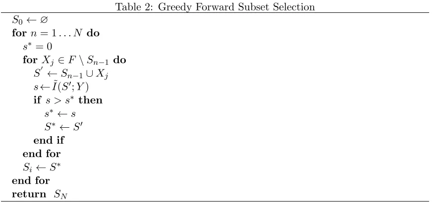
Table 2: Greedy Forward Subset Selection

S0 ←∅

for n= 1. . . N do s∗ = 0

forXj ∈F \Sn−1 do

S0 ←Sn−1∪Xj s←I˜(S0;Y) if s > s∗ then

s∗ ←s S∗ ←S0 end if end for Si←S∗

end for return SN

3.3 Greedy Forward Selection

The derived bounds and approximations provide measures for assessing the optimal set of featuresS_N∗ of sizeN. However as there are _N_!(_FF₋!_N_)! possible setsSN of sizeN finding the

optimal one by checking all the candidate sets is computationally intractable. Due to this intractability we employ a greedy optimization process in order to find a good approximation

˜

SN.

In particular, we use greedy forward selection (see table 2) to iteratively build a sequence of sets Sn withn= 1, . . . , N where each setSn is built by adding one feature Xj(n) to the previous setSn−1,i.e.Sn=Sn−1∪Xj(n). At a given iterationn, the greedy forward selection algorithm calculates for every candidate feature Xj ∈ F \Sn−1, the mutual information between the set S_n0 =Sn−1∪ {Xj} and the label Y. It then creates the set Sn by adding

that feature which leads to the largest value of the optimization criterion.

3.4 Complexity of the Gaussian Compromise Method

Though forward selection leads to a computationally tractable feature selection algorithm, it remains nonetheless very expensive. In the case of the Gaussian compromise approach, at each iteration n and for each feature Xj not in Sn−1, forward selection requires the

estimation of an approximation ofI(Sn−1∪ {Xj};Y), which in turn requires the estimation

of|Y|+ 1 determinants of the sizen×ncovariance matrices. A naive approach would be to calculate these determinants from scratch, incurring a cubic cost ofO(n3) for the calculation of each determinant and a O(|Y||F \Sn−1|n3) cost per iteration with a O(|Y|n2) memory requirement for storing the covariance matrices and their inverses.

As shown in previous work (Lefakis and Fleuret, 2014) however it is possible to de-rive both an O(|Y||F \Sn−1|n2) algorithm with O(|Y|n2) memory requirements and an

(13)

present an approach that allows for a O(|Y||F \Sn−1|n) with O(|Y|n2 +|Y||F \Sn−1|) memory requirements.

In order to speed up computations, we first note that for three random variables X,Y,

Z

I(X, Z;Y) =I(Z;Y) +I(X;Y |Z)

which in the context of our forward selection algorithm, ∀Xj ∈ F \Sn−1, and with S_n0 =

Sn−1∪ {Xj}, translates to

I(S_n0;Y) =I(Sn−1;Y) +I(Xj;Y |Sn−1).

The first term in the above expression is common for all candidate featuresXj, meaning

that finding the featureXj that maximizesI(Sn0;Y) is equivalent to finding the feature that

maximizes I(Xj;Y |Sn−1). If σ_j2_|_S_n₋₁ denotes the variance of feature j conditioned on the

features inSn−1 andσ_j2_|_y,S

n−1 the variance conditioned on the features inSn−1 and the class

Y =y, we have

argmax

Xj∈F\Sn−1

I(Xj;Y |Sn−1) = argmax

Xj∈F\Sn−1

(H(Xj |Sn−1)−H(Xj |Y, Sn−1)) (11)

= argmax

Xj∈F\Sn−1

logσ2_j_|_S_n₋₁ −X

y

P(Y =y) logσ2_j_|_y,S_n₋₁

!

(12)

where here and in the following, we slightly abuse notation and use Sn to denote both

the set and its contents, which of the two is meant will in any case be clear from context. To derive equation 12 we have exploited the fact that the conditional variance σj|Sn−1 is independent of the specific values of the features in Sn−1 and thus the integrations of the entropies over the conditioned values are straightforward. That is

H(Xj |Sn−1) =

Z

R|Sn−1|

H(Xj |Sn−1=s)µSn−1(s)ds

= 1 2logσ

2

j|Sn−1 + 1

2(log 2π+ 1).

Under the Gaussian assumption, we have

σ_j2_|_S

n−1 =σ 2

j −ΣTj,Sn−1Σ −1

Sn−1Σj,Sn−1.

From the above we can derive anO(|Y||F\Sn−1|n2) withO(|Y|n2) memory requirements by noting that computing ΣT_j,S

n−1Σ −1

Sn−1Σj,Sn−1 incurs a cost of O(n

2_{) and that this must} be done for every candidate featurej and every class y.

3.4.1 Efficient Computation of σ_j2|Sn−1

As stated, we can further speed-up the proposed algorithm by a factor of nby considering more carefully the calculation of σ_j2_|_S

n−1. IfSn−1=Sn−2∪Xi, we have

ΣT_j,S_n₋₁Σ−1_S_n₋₁Σj,Sn−1 =

h

ΣT_j,S_n₋₂σ2_ji

i

Σ−1_S_n₋₁

Σj,Sn−2.

σ2_ij

(14)

We note that ΣSn−1 differs from ΣSn−2 by the addition of a row and a column

ΣSn−1 =

ΣSn−2 Σi,Sn−2 ΣT_i,S_n₋₂ σ_i2.

Thus ΣSn−1 is the result of a rank-two update to the augmented matrix

ΣSn−2 0n−2 0T

n−2 σ2i

,

specifically a one rank-one update corresponding to changing the final row and a rank-one update corresponding to changing the final column. By applying the Sherman-Morrison formula twice to update Σ−1_S

n−2 to Σ −1

Sn−1, we can obtain

1 _{an update formula of the form}

Σ−1_S

n−1 =

"

Σ−1_S

n−2 − 1 βσ2 i u − 1 βσ2 i

uT _βσ12

i

#

+ 1

βσ2_i

u

0

uT ₀

(14)

where

u= Σ−1_S

n−2Σi,Sn−2 and

β = 1− 1

σ2_iΣ T i,Sn−2Σ

−1

Sn−2Σi,Sn−2. From equation (13) and (14) we have

σ_j2_|_S_n₋₁ =σ_j2−ΣT_j,S_n₋₁

"

Σ−1_S

n−2 − 1 βσ2 i u − 1 βσ2 i

uT _βσ12

i # + 1 βσ2 i u 0

uT 0

!

Σj,Sn−1

=σ_j2−ΣT_j,S_n₋₂Σ−1_S

n−2Σj,Sn−2 +

σ2_ji βσ2

i

uTΣj,Sn−2

−ΣT_j,S_n₋₁

" − 1 βσ2 i u 1 βσ2 i #

σ_ji2

− 1

βσ2_i

ΣT_j,S_n₋₁

u

0

uT ₀

ΣjSn−1

(15)

In eq (15) the main computational cost is incurred by the calculation of ΣT_j,S_n₋₂Σ−1_S

n−2Σj,Sn−2 which costsO(n2). However this quantity has been already calculated∀jduring the previous iteration of the algorithm since this involves calculating

σ_j2_|_S

n−2 =σ 2

j −ΣTj,Sn−2Σ −1

Sn−2Σj,Sn−2.

Thus we only need carry this result over from the previous iteration incurring an additional memory load ofO(|Y||F \Sn−1|).

The remaining terms in equation (15) can be calculated in O(n) givenβ and u. As β

and u depend only on the feature i selected in the previous iteration, remaining constant throughout iterationn, they can be pre-computed once at the beginning of each iteration. Thus the cost of calculating σ_j2_|_S

n−2 can be reduced toO(n) and the overall computational cost per iteration to O(|Y||F\Sn−1|n).

(15)

3.5 Complexity of the KL-based Algorithms

In the case of the KL-based algorithms, similarly with the Gaussian compromise approach, a naive implementation would incur a cost ofO(|Y||F\Sn−1|n3). In previous work(Lefakis and Fleuret, 2014) an algorithm was sketched which had a O(|Y|n2) memory footprint. Here we expand on this analysis and furthermore present an alternative algorithm with a

O(|Y||F\Sn−1|n) complexity, which however has an increased memory footprint (specifically

O(|Y||F \Sn−1|n2)). Working with the value:

P(Y =y)DKL(p(S|Y =y)kp(S|Y 6=y)) +P(Y =y)H(S |Y =y)

+P(Y 6=y)DKL(p(S|Y 6=y)kp(S|Y =y)) +P(Y 6=y)H(S |Y 6=y) +c000

we note that the entropy valuesH(S|Y =y) can be computed efficiently as in the previous subsection. What remains is to efficiently compute the Kullback-Leibler divergences for each of the |Y|binary classification problems.

As both distributions are assumed to be Gaussians, DKL(p(S|Y 6=y)kp(S|Y =y)) is

equal to 1 2  tr

Σy_S0

n

−1 ΣY\y

S0n

−log

|ΣY\y

S0n

|

|Σy

S0n

| +

µY\y S0n

−µy Sn0

T

Σy

Sn0

−1

µY\y S0n

−µy S0n

− |S|



.

In the following we show how each of these terms can be computed in time O(n).

3.5.1 The Term log |ΣY\y

Sn0

|

|Σy

Sn0

|

From the chain rule,

H(Sn−1∪Xj) =H(Sn−1) +H(Xj |Sn−1)

we have

log|Σ_S0

n|+

n

2 (1 + log 2π) = log|ΣSn−1|+

n−1

2 (1 + log 2π) + logσ 2

j|Sn−1+ 1

2(1 + log 2π) log|Σ_S0

n|= log|ΣSn−1|+ logσ

2

j|Sn−1

|Σ_S0

n|=σ

2

j|Sn−1|ΣSn−1|.

As shown in the previous section, the term σ_j2_|_S

n−1 can be computed in O(n) time. The term |ΣSn−1| is independent of j and can be efficiently pre-computed from |ΣSn−2| prior to iteration n using the matrix determinant lemma. By extension, the cost of calculating

log |ΣY\y

Sn0

|

|Σy

Sn0

(16)

3.5.2 Calculating Σy_S0

n

−1

Setting, here and in the rest of this section, ΣS = Σy_S for ease of exposition2 , we have

similar to section 3.4 that

Σ−1_S0

n =

"

Σ−1_S

n−1 − 1 βσ2 j u − 1 βσ2 j

uT _βσ12

j # + 1 βσ2 j u 0

uT 0 (16)

where

u= Σ−1_S

n−1Σj,Sn−1 and

β= 1− 1

σ2_jΣ T j,Sn−1Σ

−1

Sn−1Σj,Sn−1.

Here u and β cannot be pre-computed as they are different ∀j. They can either be calculated from scratch in O(n2) or, if we are willing to incur a memory overhead of O(n), withO(n) complexity from the product Σ−1_S

n−2Σj,Sn−2 which has been computed during the previous iteration (as in section 3.4.1).

3.5.3 The Term

µY\y Sn0

−µy Sn0

T

Σy

Sn0

−1

µY\y S0n

−µy Sn0

Having computedu and β as defined above, we can efficiently calculate the product

M =

µY\y Sn0

−µy Sn0

T

Σ−1

Sn0

µY\y Sn0

−µy Sn0

given thatµy S0n

=

"

µy_S_n₋₁ µy_j

#

by decomposing it as follows

M =

µY_S\y

n−1 −µ

y Sn−1

T

Σ−1_S

n−1

µY_S\y

n−1 −µ

y Sn−1

−

µY_j\y−µy_j βσ_j2 u

T_µY\y Sn−1−µ

y Sn−1

+

µY_S\y

n−1 −µ

y Sn−1

T

" ₋ 1

βσ2 j u 1 βσ2 j #

µY_j \y−µy_j

+ 1 βσ2 j

µY_S\y

n−1−µ

y Sn−1

T _u

0

uT 0

µY_S\y

n−1−µ

y Sn−1

Of these four terms, the final three involving the vectorsuand β can be calculated inO(n) as they only involve inner products. The first term requires O(n2), however as the term is independent ofj it can be calculated once at the beginning of each iteration. Consequently

the complexity of calculating µY\y Sn0

−µy Sn0

T

Σ_S0

n

−1_µY\y Sn0

−µy Sn0

givenu and β isO(n).

(17)

3.5.4 The Term tr

Σy_S0

n

−1 ΣY\y

S0n

The term tr

Σy_S0

n

−1 ΣY\y

S0n

involves calculating, and summing, the main diagonal elements

of the matrix productΣy_S0

n

−1 ΣY\y

Sn0

. We have that

ΣY_S0\y

n =





ΣY_S\y

n−1 Σ

Y\y j,Sn−1 ΣY_j,S\y

n−1

T

σY_j \y2



. (17)

From equations (16) and (17) we see that the product can be decomposed into two parts. For the first

"

Σ−1_S

n−1 − 1

βσ2

j

u

− 1

βσ2_ju

T 1

βσ_j2

#



ΣY_S\y

n−1 Σ

n−1

T

σY_j \y2





it is straightforward to show that the main diagonal elements can be calculated in O(n) provided we have pre-computed the main diagonal elements of Σ−1_S

n−1Σ

Y\y

Sn−1. As this product does not depend onjthis can be done prior to the beginning of the iteration. For the second we have

1

βσ2

j

Σ−1_S

n−1Σj,Sn−1 0

_h

ΣT_j,S

n−1Σ −1

Sn−1 0

i 



ΣY_S\y

n−1 Σ

n−1

T

σY_j\y2





which, given that tr(wTwA) = tr(wAwT), is equal to the product of _βσ12

j

and the trace of

ΣT_j,S_n₋₁Σ−1_S

n−1Σ

Y\y Sn−1Σ

−1

Sn−1Σj,Sn−1.

As we have already calculated the vector Σ−1_S

n−1Σj,Sn−1 when calculating Σ −1

Sn0

we concentrate

here on calculating the vector ΣT_j,S

n−1Σ −1

Sn−1Σ

Y\y Sn−1. As shown, the matrix Σ−1_S

n−1 can be written in the form

Σ−1_S

n−1 =

Σ−1_S

n−2 γv

γvT −γ

−γ v 0

vT ₀

where

v= Σ−1_S

n−2Σi,Sn−2 and

γ =− 1

βσ2_j.

Thus the vector ΣT_j,S_n₋₁Σ−1_S

n−1Σ

Y\y

Sn−1 can be decomposed into

ΣT_j,S_n₋₁

Σ−1_S

n−2 γv

γvT −γ

ΣY_S\y

n−1 −γΣ

T j,Sn−1

v

0

vT 0 ΣY_S\y

(18)

As v does not depend on j the product vT 0 ΣY_S_n\₋₁y can be computed prior to the

iteration and by extension the productγΣT j,Sn−1

v

0

vT ₀

ΣY_S\y

n−1 can be computed in

O(n). This leaves the final term

ΣT_j,S_n₋₁

Σ−1_S

n−2 γv

γvT −γ

ΣY_S\y

n−1.

We note that the vector ΣT_j,S_n₋₁

Σ−1_S

n−2 γv

γvT −γ

has the form

"

Σj,Sn−2Σ −1

Sn−2+γσ 2

jivT γΣT

j,Sn−2v−γσ 2

ji

#T

.

Thus we have

h

Σj,Sn−2Σ −1

Sn−2Σ

Y\y Sn−2 0

i

+γσ2_ji

vT 0

ΣY_S\y

n−1 +

γΣT_j,S_n₋₂v−γσ_ji2ΣY_i,S\y

n−1.

During the previous iteration we have already computed the vector Σj,Sn−2Σ −1

Sn−2Σ

Y\y Sn−2 and thus if we use O(n) memory to store it between iterations, we can also compute this final term inO(n).

4. Using the Eigen-decomposition to Bound Computations

The fast implementation of the GC-approximation method presented in 3.4 requires at iterationn the calculation, for each featureXj ∈F \Sn−1, of the conditioned variance

σ_j2_|_S

n−1 =σ 2

j −ΣTjSn−1Σ −1

Sn−1ΣjSn−1.

As shown, each such computation can be done inO(n). The main computational cost comes from the calculation of ΣT_jS

n−1Σ −1

Sn−1ΣjSn−1. Thus it would be advantageous to acquire a “cheap” (independent ofn) bound which will allow us to skip the calculation of this quantity for certain non-promising features.

We note that Σ−1_S

n−1 is positive definite and symmetric and thus can be decomposed as Σ−1_S

n−1 =UΛU

T_,

whereU is orthonormal and Λ is a diagonal matrix with positive elements. Thus

ΣT_jS_n₋₁Σ−1_S

n−1ΣjSn−1 = Σ

T

jSn−1UΛU

T_Σ jSn−1. As U is orthonormal we have

kΣjSn−1k2 =kΣ

T

jSn−1Uk2 =kU

T_Σ

jSn−1k2.

Symbolizing the eigenvalues as λ1, λ2, . . . , λn−1 and the elements of the vector ΣT_jS_n₋₁U as

x1, x2, . . . , xn−1, we have that

kΣT_jS_n₋₁k2₂min

i λi ≤Σ T jSn−1Σ

−1

Sn−1ΣjSn−1 ≤ kΣ

T jSn−1k

2 2max

(19)

Equation 18 gives us a bound, computable in O(|Y|), which we can use to avoid unnec-essary computations. Specifically, during iteration nof the algorithm, after having already calculated the scores of a subset of features, we have a candidate for best feature which has a score ofs∗; for each subsequent candidate featureXj we can compute the following upper

bound on the feature’s score

ub1(Xj) = log

σ_j2− kΣT_jS_n₋₁k2₂max

i λi

−

|Y|−1

X

y=0

log

σ_jy2− kΣy_jST

n−1k 2 2min_i λ

y i

, (19)

where λi, λyi are the eigenvalues of Σ

−1

Sn−1 and Σ

y−1

Sn−1 respectively. Then if ub(s) ≤s ∗_{, we}

can avoid theO(|Y|n) computations required to estimate the feature’s scores.

Furthermore shouldub1(Xj)> s∗ we can still proceed with the computations in a greedy

manner. That is instead of calculating the exact score

log

σ2_j_|_S_n₋₁

−

|Y|−1

X

y=0

log

σ_jy_|2_S

n−1

incurring O(|Y|n) cost, we can compute the conditional variances one at a time and then reassess the upper bound. That is we first calculate σ_j2_|_S

n−1 which costs us O(n) and then re-estimate the upper bound as

ub2(Xj) = log

σ_j2_|_S

n−1

−

|Y|−1

X

y=0

log

σ_jy2− kΣy_jST

n−1k 2 2min i λ y i

re-checking whether ub(s)≤s∗. We can then continue, if necessary, by calculating

ub3(Xj) = log

σ2_j_|_S_n₋₁

−log σy 2 0

j|Sn−1

−

|Y|−1

X

y=1

log

σ_jy2 − kΣy_jST

n−1k 2 2min_i λ

y i

and so forth. Thus we can avoid estimating a number of conditional variances, incurring a smaller cost. This process can continue greedily by computingub1...|Y|+1(Xj).

We note that the upper bound 19 involves |Y|lower bounds

log

σ_jy2 − kΣy_jST

n−1k 2 2min_i λ

y i

on the conditional variances σy_j_|2_S

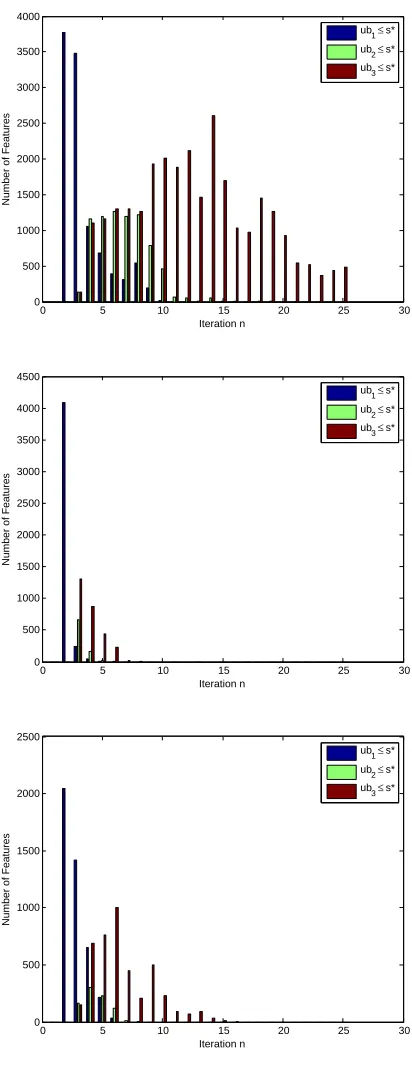
n−1. As such the bound can become quite loose if the number of classes|Y|is large. In order to empirically evaluate the usefulness of this bound in pruning computations, we considered 3 binary classification tasks; the binary task of the INRIA data set, and two tasks resulting from the CIFAR and STL data sets by a random partitioning of the classes (i.e. that is in each case 5 classes were randomly chosen to be labeled as positive and the rest as negative).

(20)

0 5 10 15 20 25 30 0

500 1000 1500 2000 2500 3000 3500 4000

Iteration n

Number of Features

ub

1≤ s*

ub

2≤ s*

ub₃≤ s*

0 5 10 15 20 25 30

0 500 1000 1500 2000 2500 3000 3500 4000 4500

Iteration n

Number of Features

ub₁≤ s*

ub

2≤ s*

ub₃≤ s*

0 5 10 15 20 25 30

0 500 1000 1500 2000 2500

Iteration n

Number of Features

ub₁≤ s*

ub

2≤ s*

ub

3≤ s*

Figure 3: Number of features for which the upper boundubxallows us to skip computations

(21)

can avoid all computations concerning the conditional variances. In the caseub2 ≤s∗ only one conditional variance need be calculated, while in the case of ub3 ≤ s∗ two (out of a possible three). As can be seen, the bound can prove quite useful in pruning computations, as is the case in the INRIA data set. For the CIFAR data set, we see that the bound can still prove useful, especially early on. On the contrary in the case of the STL data set, the bound seems to provide little help in ways of avoiding computations.

Pruning computations using the above bounds requires access to the eigenvalues of the matrices Σy_S−1

n−1 which are the reciprocals of the eigenvalues of the matrices Σ

y Sn−1. As computing the eigen-decomposition of a matrix, from scratch, can be expensive we present in the following a novel algorithm for efficiently calculating these eigenvalues, and the corresponding eigenvectors, of Σy_S−1

n−1 from the eigen-decomposition of Σ

y−1

Sn−2.

4.1 Eigen-system Update

The matrices Σy_S−1

n−1 results from the matrices Σ

y−1

Sn−2 by the addition of a row and a column. We are faced thus with the problem of updating the eigen-system of a symmetric and positive definite matrix Σ when a vector is inserted as an extra row and column.

More specifically, we shall present a method for efficiently computing the eigen-system

Un+1,Λn+1 of a (n+ 1)×(n+ 1) matrix Σn+1 when the eigen-systemUn,Λn of then×n

matrix Σn is known and Σn+1 is related to Σn as follows: Σn+1 =

Σn v vT c

,

wherevandcare such that the matrix Σn+1 is positive definite. Without loss of generality, we will consider in the following the special casec= 1.

Ifun₁, . . . ,un_n andλn₁, . . . , λn_n are the eigenvectors and respective eigenvalues of Σn, then

un_i

0

is obviously an eigenvector of

Σ0 =

Σn 0 0T 1

,

with associated eigenvalueλ0i=λni. Also, if∀i∈ {1, . . . , n+ 1},ei is theithstandard basis

vector of Rn+1, then Σ0en+1 =en+1 and en+1 is an eigenvector of Σ0 with a corresponding eigenvalue of λ0n+1 = 1.

The matrix Σn+1 can be expressed as the result of a rank-two update to Σ0 Σn+1= Σ0+en+1

v

0

T

+

v

0

eT_n₊₁.

IfU0,Λ0 denote the eigen-system of Σ0, by multiplying

Σn+1un+1=λn+1un+1,

on the left byU0T, we have

U0T Σ0+en+1

v

0

T

+

v

0

eT_n₊₁ !

(22)

Given that Σ0 is positive definite and symmetric it follows that U0U0T =I and

U0T Σ0+en+1

v 0 T + v 0 eT_n₊₁

!

U0U0Tun+1 =λn+1U0Tun+1

and since U0TΣ0U0 = Λ0 we have

Λ0+en+1qT +qeTn+1

U0Tun+1=λn+1U0Tun+1

whereq =U0T

v

0

, noteeT_n₊₁U0 =eT_n₊₁.

Thus Σn+1and the matrix Σ00 = Λ0+en+1qT +qeTn+1

share eigenvalues. Furthermore the eigenvectors Un+1 are related to the eigenvectorsU00 of Σ00 by Un+1 =U0U00.

4.1.1 Computing the Eigenvalues and Eigenvectors of Σ00

The matrix Σ00 has non-zero elements only on its main diagonal and on its last row and column. By developing the determinant |Σ00−λI|along the final row we have

|Σ00−λI|=Y

j

(λ0_j−λ) + X

i<n+1



−q2_i Y

j6=i,j<n+1

(λ0_j−λ)



,

where qi is the ith element of vector q. The determinant thus has the same roots as the

function

f(λ) = |Σ 00₋_λI_|

Q

j<n+1(λ 0

j−λ)

(20)

= λ0n+1−λ+

X

i

−q_i2

(λ0i−λ)

. (21)

We have ∀i, lim

λ−→>λ0

if(λ) = +

∞ and lim

λ−→< λ0

if(λ) =

−∞. Furthermore we have

∂f(λ)

∂λ =−1 +

X

i

−q_i2

(λ0i−λ)2

≤0

meaning the function f is strictly decreasing between its poles. From this and from the positive definiteness of Σ00 we have that

0< λn₁+1 < λ01< λ₁n+1<· · ·< λ0n+1 < λn_n+1₊₁ i.e. the eigenvalues of Σ0 and Σ00 are interlaced.

Though there is no analytical solution for finding the roots of f(λ), given the above relationship they can be computed efficiently using a Householder method. We also note that tr(Λ0) = tr(Σ00) and consequently

λn_n+1₊₁=X

i λ0i−

X

i<n+1

(23)

Once we have computed the eigenvalues λ00, we can compute the eigenvectors U00 as follows: we first note that ∀kthe system of linear equations

Σ00x=λn_k+1x

where

x=

x1 x2 . . . xn+1

T

involvesn equations of the form

λ0ixi+qixn+1 =λnk+1xi.

Given that λn_k+1 6=λ0i it follows that if xn+1 = 0 then ∀i, xi = 0 and thus it must be

that xn+1 6= 0. As the system has one degree of freedom, we can set xn+1 = 1. We then have from the equations

λ0ixi+qixn+1=λnk+1xi

that

xi= qi λn_k+1−λ0

i ,

and by normalizing x we obtain the kth column of U00. Finally we can obtain the

eigen-decomposition of Σn+1

Σn+1 = (U0U00)Λ00(U0U00)T.

4.1.2 Computational Efficiency

In order to empirically evaluate the derived eigen-decomposition update algorithm, we com-pare a C++ implementation against the LAPACK library’s eigen-decomposition implemen-tation. In figure 4.1.2 we see such a comparison of the CPU time required to compute Σn+1, from scratch, using the LAPACK library and using the proposed update algorithm, as a function of n.

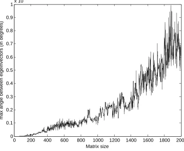
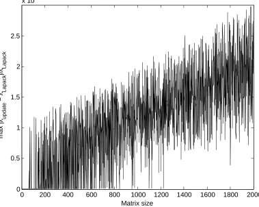
4.1.3 Numerical Precision

In order to test the numerical precision of the proposed update method, we consider two experimental setups. In the first setup, results on which are shown in figures 5,6, we it-eratively augment a symmetric positive definite matrix by inserting a vector as an extra row and an extra column and at each iteration update its eigen-decomposition using the proposed method; that is to say at each iteration the eigen-decomposition is an updated version of previously updated decompositions. Figure 5 shows the maximum relative eigen-value error as compared to the decomposition estimated by LAPACK which is assumed to be accurate. Similarly figure 6 shows the maximum angle between corresponding eigenvec-tors of the proposed method and the ones computed by the LAPACK library. As can be seen, after 2000 iterations the maximumrelative eigenvalue error is of the order of magni-tude of ∼ 1%, while the maximum angle between corresponding eigenvectors is less than 0.001 degrees.

(24)

0 200 400 600 800 1000 1200 1400 1600 1800 2000 0

5 10 15 20 25 30

CPU time in secs

Matrix size Lapack

Update

(25)

As can be seen the maximum relative error is of the order of magnitude of 10−10. this value is related to the tolerance of the Newton method which was used to find the roots of equation 20 (which in these experiments we set to 10−10). The maximum angle between corresponding eigenvectors was found to be 0,i.e. beneath double precision, in every case.

5. Experiments

In this section we present an empirical evaluation of the proposed algorithms. We first show on a synthetic controlled experiment that they behave as expected regarding groups of jointly informative features, and then provide results obtained on three popular real-world computer vision data sets.

5.1 Synthetic Examples

In order to show the importance of joint informativeness and the ability of the proposed algorithm to capture it we construct a simple synthetic experiment with a set of candidate features F ={X1, X2, X3, X4, X5}defined as follows:

X1 ∼ N(0,1) + 10−1Y

X2 ∼ (2Y −1)X1 +N(0,1)

X3 ∼ N(0,1)

X4 ∼ N(0,1) + 10−1Y

X5 ∼ (2Y −1)X4+N(0,1)

where Y is a classification label, Y ∼ B(0.5). Looking at the above marginals it can be seen that only X1 and X4 carry information regarding Y individually,X2 and X5 are very informative but only in conjunction with X1 and X4 respectively. X3 is simply noise.

We generate 1,000 synthetic data sets of 25,000 data points each from the above distri-butions, and use the GC-approximation on the mutual information to select the features. In 49.2% of the experiments the algorithm ranksX1 as the most informative feature. Even though X4 would be the second most informative feature marginally, in every one of these experiments in the second iteration the algorithm chose theX2 feature as it is jointly more informative when combined withX1. Similarly, in 47.1% of the experiments the algorithm ranked X4 first and in each of these experiments selected X5 second. In every one of the runsX3 was ranked as the least informative of the 5 features.

5.2 Data Sets

We report results on three standard computer vision data-sets which we used for our ex-periments:

CIFAR-10 contains images of size 32×32 of 10 distinct classes depicting vehicles and animals. The training data consists of 5,000 images of each class. We pre-process the data as in (Coates and Ng, 2011) using the code provided by the authors. The original pool F

(26)

0 200 400 600 800 1000 1200 1400 1600 1800 2000 0

1 2 3 4 5 6 7 8

9x 10

−3

Matrix size

max |

λ update

−

λ Lapack

|/

λ Lapack

(27)

0 200 400 600 800 1000 1200 1400 1600 1800 2000 0

0.1 0.2 0.3 0.4 0.5 0.6 0.7 0.8 0.9

1x 10

−3

Matrix size

max angle between eigeinvectors (in degrees)

(28)

0 200 400 600 800 1000 1200 1400 1600 1800 2000 0

0.5 1 1.5 2 2.5

x 10−10

max |

λ update

−

λ Lapack

|/

λ Lapack

Matrix size

(29)

INRIA is a pedestrian detection data set. There are 12,180 training images of size 64×128 of pedestrians and background images. We use 3,780 HoG features that have been shown to perform well in practice (Dalal and Triggs, 2005).

STL-10 consists of images of size 96×96 belonging to 10 classes, each represented by 500 training images. As for CIFAR we pre-process the data as in (Coates and Ng, 2011), resulting in a pool F of 4,096 features.

5.3 Baselines

We compare the proposed feature selection methods against a number of baselines. The Fisher, T-test, χ2, and InfoGain methods all compute statistics on individual features. In particular InfoGain calculates the mutual information of the individual features to the class, without taking into account their joint informativeness. As such, its comparison with our approaches is a very good indicator of the merit of joint informativeness and its effect on classification performance.

As noted in section 2, the FCBF (Liu and Yu, 2003) and CFS (Hall and Smith, 1999) baselines employ symmetric uncertainty criteria and check for pairwise redundancy of features. SimilarlyMRMR (Peng et al., 2005), uses mutual information to select features that have high relevance to the class while having low mutual information with the other selected features, thus checking for pairwise informativeness. Comparison with the proposed methods proves the importance of going beyond pairwise redundancy.

The RelieFF baseline (Robnik-ˇSikonja and Kononenko, 2003) looks at the nearest neighbors of random samples along the individual features. In order to compare with spectral clustering approaches we show results for (Wolf and Shashua, 2005), marked as Spectral in the tables, which we found to outperform (Zhao and Liu, 2007) in practice. Finally, we also show results for three wrapper methods, namely SBMLR (Cawley et al., 2006), which employs a logistic regression predictor,CMTF (Argyriou et al., 2008) which uses a sparsity inducingl1-norm, andGBFS (Xu et al., 2014) which uses gradient boosted trees.

We compare these baselines against the four methods proposed here, namely maximizing the entropy (GC.E) or the mutual information (GC.MI) under the Gaussian compromise approximation, and maximizing the KL-based entropy (GKL.E) and mutual information (GKL.MI). In the case of the GC methods, when an iteration is reached where for all candidate features and for all classes the prior over the class variable is lower than the entropy of f∗, we halt the GC-approximation feature selection procedure and randomly select the remaining features.

5.4 Results

In tables 4, 5, 6, and 7, we show experimental results for the three data sets. In order to show the general applicability of the proposed methods, we combined the selected features with four different classifiers: AdaBoost with classification stumps, linear SVM, RBF-kernel SVM, and quadratic discriminant analysis (QDA). We show results for several numbers of selected features {10,25,50,100}.

(30)

from these tables,GC.MIand GKL.E consistently rank amongst the top three methods, with GC.MI ranking in the top three 24 out of 48 times and first 8 times, and GKL.E being in the top three 27 out of 48 times and first 11 times. The only other comparable methods are SBMLR which ranks in the top three 17 out of 48 times and first 10 times andGBFS which ranks in the top three 20 out of 48 times and first 5 times. We note that both of these methods are wrapper methods.

Furthermore as can be seen in table 3, the running time of the proposed methods3 is very competitive with respect to the more complex feature selection algorithms. The Gaussian Compromise algorithms are especially fast as they are two orders of magnitude faster than practically all other methods. We especially note that the SBMLR method which performs comparably in terms of accuracy is very slow when compared to GC.MI. Though theMRMRalgorithm is faster than GC.MIon the INRIA data set, it performs considerably worse accuracy-wise on that data set; on the data sets where it does perform well (e.g. CIFAR) it is considerably slower than GC.MI. We also note that the GBFS method is quite slower than GC.MI.

The computation times provided were obtained with C++ implementations of the pro-posed methods. TheMRMR algorithm is also implemented in C++, while theSpectral and CMTF baselines are implemented in MATLAB, as both these algorithms mainly use matrix algebra we believe these timings to be indicative. The remaining algorithms were implemented in Java. As noted in (Bouckaert et al., 2010) these implementations should be competitive in speed with C++ implementations.

FCBF MRMR SBMLR Spectral GBFS CFS CMTF RelieFF GC.MI GKL.E

CIFAR 621 56 1449 1379 95 4262 394 1652 20 486

STL 68 20 1002 367 41 409 208 2089 5 887

INRIA 247 32 88 1072 233 2516 459 2413 43 135

Table 3: (Approximate) Cost in CPU time of running the more sophisticated feature selec-tion algorithms in order to select 100 features on the three data sets. We highlight in bold the fastest algorithm for each data set.

5.5 Finite Sample Analysis

The proposed methods all depend on the covariance matrices Σ, Σy. Of course, in practice, one rarely has access to the true covariance matrices of the underlying distributions but rather estimates based on using finite sets of samples. Given aN×DmatrixP where each row is a sample from the underlyingD-dimensional distribution, we symbolize

ˆ ΣN =

1

NP T_P

the empirical estimation ˆΣN of matrix Σ, computed from these N samples. The accuracy

of this approximation is important to the success of the proposed methods. It can be shown

(31)

CIFAR STL INRIA

AdaBoost 10 25 50 100 10 25 50 100 10 25 50 100

Fisher 29.23 36.96 42.07 49.06 31.86 35.78 39.72 41.81 86.90 89.83 90.38 91.45

FCBF 37.77 44.42 51.15 54.83 33.25 38.05 39.87 42.81 90.87 94.02 95.44 94.67 MRMR 39.42 45.84 49.76 54.85 32.24 39.61 40.61 43.00 81.53 88.48 93.48 94.91

χ2 28.13 35.54 43.68 49.46 29.61 36.88 39.39 41.89 92.81 93.11 93.94 94.91

SBMLR 34.87 45.08 52.17 56.70 34.22 41.26 44.65 47.15 86.40 87.50 88.04 88.06

tTest 25.74 31.30 36.57 43.16 31.74 34.75 39.31 42.34 85.01 88.41 88.84 91.70

InfoGain 29.01 35.90 40.20 48.34 31.13 36.60 38.62 42.03 92.58 93.29 93.96 94.93

Spectral 19.90 25.13 33.18 40.44 19.06 26.30 33.52 38.51 92.78 93.69 93.92 94.83

RelieFF 28.13 34.64 40.85 47.70 33.91 37.46 42.79 45.22 91.79 95.44 95.83 96.43

CFS 33.50 38.96 44.58 54.22 30.75 38.40 41.85 44.39 89.69 92.60 96.41 97.69

CMTF 21.79 31.98 39.43 45.23 28.70 33.55 34.71 36.86 80.01 83.72 92.55 95.58

GBFS 32.02 40.20 48.87 54.34 30.96 38.56 42.30 45.57 93.90 95.87 96.90 97.66

GC.E 32.45 42.54 50.15 55.06 31.86 37.41 42.19 46.99 89.54 90.09 94.30 95.81

GC.MI 36.47 44.55 51.44 55.39 36.50 40.79 43.82 44.39 95.04 95.87 96.68 97.30 GKL.E 37.51 46.41 52.11 56.41 34.76 39.71 43.49 46.46 89.92 91.84 94.14 96.63

GKL.MI 33.71 40.04 47.17 51.12 33.00 38.80 42.13 43.58 92.18 93.09 95.21 96.15

Table 4: Test accuracy of an AdaBoost classifier trained on a different number of selected features{10,25,50,100} on the three data sets.

CIFAR STL INRIA

SVMLin 10 25 50 100 10 25 50 100 10 25 50 100

Fisher 25.19 33.53 39.47 48.12 26.09 30.79 34.63 38.02 92.55 93.73 94.03 94.68

FCBF 33.65 42.02 47.77 54.97 31.74 34.85 38.11 40.66 94.14 96.03 96.03 96.03 MRMR 35.48 42.5346.02 52.64 32.50 39.06 43.69 49.36 79.85 84.18 91.73 93.91

χ2 21.77 32.06 40.65 48.58 22.61 31.82 34.29 37.96 92.94 93.27 93.50 94.61

SBMLR 30.43 42.60 51.41 56.81 32.29 38.26 43.29 47.15 85.92 87.95 88.57 88.64

tTest 25.69 32.56 40.17 45.12 26.72 29.95 36.23 39.14 80.01 87.21 87.64 89.23

InfoGain 24.79 32.32 37.98 47.37 27.17 31.82 33.70 37.84 92.35 93.08 93.75 94.68

Spectral 17.19 23.14 32.78 42.60 18.91 26.55 32.65 38.24 92.67 93.57 93.64 94.44

RelieFF 24.56 30.60 38.17 46.51 29.16 32.40 38.05 42.94 90.99 95.04 95.97 96.36

CFS 31.49 36.46 42.17 51.70 28.63 34.45 38.54 41.88 88.64 91.68 96.11 97.53

CMTF 21.10 31.64 40.39 47.71 27.61 34.81 38.99 42.32 79.09 80.29 89.49 93.01

GBFS 28.37 38.18 45.89 52.36 30.78 39.29 45.06 50.39 76.79 92.55 95.38 97.03

GC.E 28.76 41.14 48.70 55.16 31.20 37.60 43.31 49.75 87.73 87.67 91.96 93.13

GC. MI 34.02 42.1449.16 55.07 32.50 39.75 44.15 48.88 89.76 93.09 95.71 96.45 GKL.E 32.39 43.26 50.12 55.02 33.44 38.6244.27 50.54 85.31 89.46 92.05 96.36

GKL. MI 28.67 34.65 43.30 48.69 32.16 39.35 44.87 47.96 85.66 90.99 92.14 95.16

Table 5: Test accuracy of a linear SVM trained on a different number of selected features

(32)

CIFAR STL INRIA

SVM-RBF 10 25 50 100 10 25 50 100 10 25 50 100

Fisher 29.11 39.22 46.05 54.68 34.71 40.13 43.87 45.77 92.44 93.55 93.38 92.97

FCBF 40.48 51.15 57.73 64.26 38.86 43.35 46.06 47.20 88.29 93.91 92.60 95.66 MRMR 41.80 51.97 57.31 62.14 38.39 44.87 47.02 48.92 80.07 79.99 88.89 90.48

χ2 _{27.16 38.23 47.60 54.70 32.53 41.27 43.22 44.88} _92.78 _{93.16 93.02 93.25}

SBMLR 36.06 49.83 60.32 64.97 32.29 38.26 43.29 47.15 82.82 86.05 87.39 87.14

tTest 28.68 35.75 41.89 49.13 34.30 38.73 44.30 45.90 80.01 87.00 87.11 87.32

InfoGain 29.21 38.68 43.92 53.94 35.57 41.23 42.92 45.12 92.28 92.71 93.01 93.38

Spectral 22.89 30.92 40.41 49.75 24.80 32.91 40.11 43.70 92.67 93.09 92.85 93.29

RelieFF 29.49 37.08 45.39 53.96 38.22 42.36 47.27 50.35 90.62 94.56 95.05 95.20

CFS 35.50 43.74 50.98 61.01 35.32 42.72 47.46 49.82 88.34 91.31 95.44 97.14

CMTF 23.90 36.74 45.51 52.86 31.80 36.94 38.06 39.65 80.01 83.72 92.55 93.68

GBFS 34.98 45.07 54.70 61.27 33.65 43.99 49.04 51.52 93.00 95.25 95.83 96.48

GC.E 35.29 51.12 60.34 65.76 36.16 42.64 45.37 47.79 87.73 87.67 91.96 93.13

GC. MI 39.57 49.91 57.79 64.32 35.86 43.35 45.80 47.81 94.26 94.17 94.44 95.76 GKL.E 39.84 52.80 60.94 65.64 39.67 46.31 50.06 52.89‘ 86.01 88.94 92.79 95.43

GKL. MI 34.49 43.09 51.48 56.54 35.95 41.65 45.27 45.86 91.03 91.91 93.36 93.98

Table 6: Test accuracy of a SVM with a RBF kernel when trained on a different number of selected features{10,25,50,100} on the three data sets.

CIFAR STL INRIA

QDA 10 25 50 100 10 25 50 100 10 25 50 100

Fisher 25.41 33.31 39.67 47.53 34.73 39.91 44.24 48.35 87.41 88.63 89.17 91.31

FCBF 35.02 43.97 52.32 58.99 37.44 41.89 45.70 48.89 89.95 94.00 94.00 94.00 MRMR 36.19 44.54 48.22 53.88 36.89 42.84 46.44 49.90 62.98 76.56 86.84 90.60

χ2 _{21.81 31.85 39.39 47.75 32.71 40.45 43.64 47.25 87.85 88.20 89.30 91.75}

SBMLR 31.71 43.46 53.31 58.86 36.89 45.26 49.58 51.65 76.30 80.36 81.00 81.49

tTest 26.34 33.39 39.16 45.33 33.92 40.09 45.05 47.63 76.16 82.50 82.85 85.23

InfoGain 22.38 31.61 37.65 46.47 34.17 40.94 44.51 47.81 87.99 88.08 89.49 91.77

Spectral 17.97 24.80 34.99 44.25 25.39 35.45 44.39 49.68 87.99 88.26 89.07 91.26

RelieFF 24.61 29.67 38.20 47.18 37.57 42.59 47.60 50.92 83.38 92.14 93.16 94.24

CFS 31.50 36.18 42.93 52.92 34.06 42.29 48.45 51.09 83.79 88.31 94.00 96.66

CMTF 20.61 31.98 41.04 48.60 33.76 43.04 47.51 51.02 61.04 72.31 89.23 92.67

GBFS 29.48 38.39 46.86 53.84 34.92 42.83 47.89 51.26 91.19 91.35 94.15 96.02

GC.E 31.01 44.10 53.21 58.41 33.76 43.04 47.51 51.02 85.06 86.31 91.22 94.10

GC. MI 33.68 43.02 51.84 58.43 35.31 42.24 47.21 49.88 92.14 94.08 95.07 96.31 GKL.E 34.06 44.21 53.29 57.98 37.39 43.30 47.39 51.82 79.30 86.21 90.83 95.74

GKL. MI 29.06 35.10 42.50 46.24 33.56 40.02 45.07 46.44 85.09 88.03 91.72 94.84

(33)

(see theorem 5.39 in (Vershynin, 2012)) that in the case of a matrix with (sub)-Gaussian generated rows, we have ∀t≥0 with probability at least 1−2e−ct2

kΣˆN−Σk ≤max(δ, δ2),

where

δ = C

√

D+t

√

N

andc,Care constants related to the sub-Gaussian norm of the rows ofP. Replacingtwith

C0t√Din the above (see Corollary 5.50 in Vershynin (2012)), we have, for sufficiently large

C0,∀∈(0,1), and ∀t≥1 with probability at least 1−2e−ct2

If N ≥C(t/)2D then kΣˆN−Σk ≤.

Thus N =O(D) samples are needed to sufficiently approximate the covariance matrix by the finite sample covariance matrix when the underlying distribution is sub-Gaussian, compared to O(DlogD) for an arbitrary distribution (Corollary 5.52 (Vershynin, 2012)).

Based in this, in order to select dfeatures, the proposed methods theoretically require

O(d) samples. This however assumes that the feature selection methods depend solely on the covariance matrices Σ. This holds true only for the GC-approximation in section 3.2.1, the KL-based bound depends both on Σ and Σ−1. Furthermore, as shown in section 3.4, the more efficient implementation of the GC-approximation also depends on Σ−1.

Unfortunately, estimating the precision matrix by taking the inverse of the sample co-variance matrix is known to be unstable (Cai et al., 2016). Though a number of methods have been proposed to address this issue (Cai et al., 2011), their complexity makes them unsuitable in the present setting. To investigate whether this instability affects the perfor-mance of the proposed methods, we present in the following an empirical analysis of the effect of sample size on prediction performance.

5.5.1 Empirical Evaluation

In order to assess the influence of sample set size on performance, we consider the accuracy on the test set of a linear SVM. Specifically we perform feature selection using a subset of the training data by selecting uniformly at random without replacement. Thus the relevant sample covariance matrices are estimated using these smaller sets. We then train a linear SVM using the selected subset of features but using the entire set of samples; this is done to avoid any influence of sample size on the training of the SVM and by extension on the final results.

(34)

Similarly in figure 9 we show results for the KL-bound case. Here we see that sample size is more influential. A possible explanation is that though the feature selection method arising from the GC-approximation involves the estimation of |Y|+ 1 inverse covariance matrices, in the case of the KL-bound feature selection method involves 2|Y| inverses. Examining the plots in figure 9, we see that in the case of the STL and CIFAR data sets there is some degradation of performance for small sample set sizes, though the performance quickly reaches that of the full set as the subset size increases. In the case of the INRIA data set however we see that the method performs considerably worse when only a subset of the data set is used to perform feature selection.

6. Conclusion

The present work concentrates on developing tractable algorithms to exploit information theoretic criteria for feature selection. The proposed methods focus on feature selection in the context of classification and demonstrate that it is possible to choose features that are jointly informative by careful density modeling and algorithmic implementation. Thus the joint mutual information of variables can in fact be employed efficiently for feature selection as opposed to using only the mutual information of marginal or pairwise distributions as has typically been used in the literature.

The proposed methods rely on modeling the conditional joint distributions of the fea-tures given the class to predict and subsequently maximizing either upper bounds on the information theoretic measures or relevant approximations. To reduce the computational cost of a forward feature selection scheme incorporating these criteria, we have proposed efficient implementations for both approaches, so that they are competitive with other state-of-the-art methods in terms of speed. We have also presented a novel method for updating the eigen-decompositions of a specific family of matrices (and updates) which our GC-approximation feature selection algorithm exploits.

Empirical results show the methods to be competitive with current state-of-the-art with respect to prediction accuracy. Furthermore, an empirical analysis of the performance of these methods in connection with the number of samples in the data sets has shown them to be relatively robust in this respect.

Acknowledgments

This work was supported by the Hasler Foundation through the MASH-2 project.

References

Andreas Argyriou, Theodoros Evgeniou, and Massimiliano Pontil. Convex multi-task fea-ture learning. Machine Learning, 73(3):243–272, 2008.

(35)

0 50 100 150 200 250 300 350 400 28

30 32 34 36 38 40 42 44

Number of Samples per Class

Test Accuracy

10 features 25 features 50 features

0 500 1000 1500 2000 2500

25 30 35 40 45 50