Composite Self-Concordant Minimization
Quoc Tran-Dinh [email protected]
Anastasios Kyrillidis [email protected]
Volkan Cevher [email protected]
Laboratory for Information and Inference Systems (LIONS) ´
Ecole Polytechnique F´ed´erale de Lausanne (EPFL) CH1015-Lausanne, Switzerland
Editor:Benjamin Recht
Abstract
We propose a variable metric framework for minimizing the sum of a self-concordant func-tion and a possibly non-smooth convex funcfunc-tion, endowed with an easily computable proxi-mal operator. We theoretically establish the convergence of our framework without relying on the usual Lipschitz gradient assumption on the smooth part. An important highlight of our work is a new set of analytic step-size selection and correction procedures based on the structure of the problem. We describe concrete algorithmic instances of our framework for several interesting applications and demonstrate them numerically on both synthetic and real data.
Keywords: proximal-gradient/Newton method, composite minimization, self-concordance, sparse convex optimization, graph learning
1. Introduction
The literature on the formulation, analysis, and applications ofcomposite convex minimiza-tion is ever expanding due to its broad applications in machine learning, signal processing, and statistics. By composite minimization, we refer to the following optimization problem:
F∗ := min
x∈Rn{F(x) | F(x) :=f(x) +g(x)}, (1)
wheref andgare both closed and convex, andnis the problem dimension. In the canonical setting of the composite minimization problem (1), the functionsf andgare assumed to be smooth and non-smooth, respectively (Nesterov, 2007). Such composite objectives naturally arise, for instance, in maximum a posteriori model estimation, where we regularize a model likelihood function as measured by a data-driven smooth termf with a non-smooth model priorg, which carries some notion of model complexity (e.g., sparsity, low-rankness, etc.).
F
LF
µF
2F
2,⌫F: smooth Class Property
x,y∈dom(f), v∈Rn,0≤µ≤L <+∞
FL k∇f(x)− ∇f(y)k∗≤Lkx−yk
Fµ µ2kx−yk2+f(x) +∇f(x)T(y−x)≤f(y)
F2 |ϕ000(t)| ≤2ϕ00(t)3/2: ϕ(t) =f(x+tv), t∈R
F2,ν F2 and supv∈Rn
2∇f(x)Tv− kvk2 x ≤ν
Figure 1: Common structural assumptions on the smooth functionf.
presence of a non-smooth term g prevents direct applications of scalable smooth optimiza-tion techniques, such as sequential linear or quadratic programming.
Fortunately, we can provably trade-off accuracy with computation by further exploiting the individual structures of f and g. Existing methods invariably rely on two structural assumptions that particularly stand out among many others. First, we often assume that
f has Lipschitz continuous gradient (i.e., f ∈ FL: cf., Figure 1). Second, we assume
that the proximal operator of g (proxH
g (y) := arg minx∈
Rn
g(x) + (1/2)kx−yk2H ) is, in a user-defined sense, easy to compute for some H 0 (e.g., H is diagonal); i.e., we can computationally afford to apply the proximal operator in an iterative fashion. In this case, g is said to be “tractably proximal”. On the basis of these structures, we can design algorithms featuring a full spectrum of (nearly) dimension-independent, global convergence rates with well-understood analytical complexity (see Table 1).
Order Method example Main oracle Analytical complexity
1-st [Accelerated]a-[proximal]-gradientb ∇f,proxLIn
g [O(−1/2)]O(−1)
1+-th Proximal-quasi-Newtonc H
k,∇f,proxHg k O(log−1) or faster
2-nd Proximal-Newtond ∇2f,∇f,prox∇2f
g O(log log−1)[local]
See (Beck and Teboulle, 2009a)a,b,(Becker and Fadili, 2012)c,(Lee et al., 2012)d,(Nesterov, 2004, 2007)a,b.
Table 1: Taxonomy of [accelerated] [proximal]-gradient methods whenf ∈ FLor
proximal-[quasi]-Newton methods when f ∈ FL∩ Fµ to reach an ε-solution (e.g., F(xk)−
F∗≤).
Unfortunately, existing algorithms have become inseparable with the Lipschitz gradient assumption onf and are still being applied to solve (1) in applications where this assump-tion does not hold. For instance, when proxH
g (y) is not easy to compute, it is still possible
to establish convergence—albeit slower—with smoothing, splitting or primal-dual decom-position techniques (Chambolle and Pock, 2011; Eckstein and Bertsekas, 1992; Nesterov, 2005a,b; Tran-Dinh et al., 2013c). However, when f /∈ FL, the composite problems of the
form (1) are not within the full theoretical grasp. In particular, there is no known global convergence rate. One kludge to handle f /∈ FL is to use sequential quadratic
the optimal solution. Attempts at global convergence require aglobalization strategy such as line search procedures (cf., Section 1.2). However, neither the strong regularity nor the line search assumptions can be certified a priori.
To this end, we address the following question in this paper: “Is it possible to ef-ficiently solve non-trivial instances of (1) for non-global Lipschitz continuous gradient f
with rigorous global convergence guarantees?” The answer is positive (at least for a broad class of functions): We can still cover a full spectrum of global convergence rates with well-characterizable computation and accuracy trade-offs (akin to Table 1 for f ∈ FL)
for self-concordantf (in particular, self-concordant barriers) (Nemirovskii and Todd, 2008; Nesterov and Nemirovski, 1994):
Definition 1 (Self-concordant (barrier) functions) A convex function f :Rn→R is said to be self-concordant (i.e., f ∈ FM ) with parameter M ≥0, if|ϕ000(t)| ≤ M ϕ00(t)3/2,
where ϕ(t) :=f(x+tv) for allt∈R, x∈dom(f) and v∈Rn such thatx+tv∈dom(f). When M = 2, the function f is said to be a standard self-concordant, i.e., f ∈ F2.1 A standard self-concordant function f ∈ F2 is a ν-self-concordant barrier of a given convex set Ω with parameter ν > 0, i.e., f ∈ F2,ν, when ϕ also satisfies |ϕ0(t)| ≤√νϕ00(t)1/2 and
f(x)→+∞ as x→∂Ω, the boundary ofΩ.
While there are other definitions of self-concordant functions and self-concordant barriers (Boyd and Vandenberghe, 2004; Nemirovskii and Todd, 2008; Nesterov and Nemirovski, 1994; Nesterov, 2004), we use Definition 1 in the sequel, unless otherwise stated.
1.1 Why is the Assumption f ∈ F2 Interesting for Composite Minimization?
The assumptionf ∈ F2 in (1) is quite natural for two reasons. First, several important
ap-plications directly feature a self-concordantf, which does not have global Lipschitz continu-ous gradient. Second, self-concordant composite problems can enable approximate solutions of general constrained convex problems where the constraint set is endowed with a ν -self-concordant barrier function.2 Both settings clearly benefit from scalable algorithms. Hence,
we now highlight three examples below, based on compositions with the log-functions. Keep in mind that this list of examples is not meant to be exhaustive.
Log-determinant: The matrix variable function f(Θ) := −log detΘis self-concordant with dom(f) := {Θ∈Sp |Θ0}, where Sp is the set of p×p symmetric matrices. As a stylized application, consider learning a Gaussian Markov random field (GMRF) of p
nodes/variables from a data set D := {φ1,φ2, . . . ,φm}, where φj ∈ D is a p-dimensional random vector with Gaussian distributionN(µ,Σ). LetΘ:=Σ−1be the inverse covariance (or the precision) matrix for the model. To satisfy the conditional dependencies with respect to the GMRF,Θmust have zero in (Θ)ij corresponding to the absence of an edge between
node iand nodej; cf., (Dempster, 1972).
1. We use this constant for convenience in the derivations since iff ∈ FM, then (M2/4)f∈ F2.
2. Let us consider a constrained convex minimizationx∗C := arg minx∈Cg(x), where the feasible convex setC is endowed with aν-self-concordant barrier ΨC(x). If we letf(x) := νΨC(x), then the solution
x∗ of the composite minimization problem (1) well-approximates x∗C as g(x
∗
) ≤ g(x∗C) + (∇f(x
∗
) +
We can learn GMRFs with theoretical guarantees from as few as O(d2logp) data sam-ples, wheredis the graph node degree, via`1-norm regularization formulation (see Raviku-mar et al. 2011):
Θ∗ := arg min Θ0
n
−log det(Θ) + tr(ΣΘb )
| {z }
=:f(Θ)
+ρkvec(Θ)k1
| {z }
=:g(Θ)
o
, (2)
where ρ > 0 parameter balances a Gaussian model likelihood and the sparsity of the so-lution, Σb is the empirical covariance estimate, and vec is the vectorization operator. The
formulation also applies for learning models beyond GMRFs, such as the Ising model, since
f(Θ) acts also as a Bregman distance (Banerjee et al., 2008).
Numerical solution methods for solving problem (2) have been extensively studied, e.g. in (Banerjee et al., 2008; Hsieh et al., 2011; Lee et al., 2012; Lu, 2010; Olsen et al., 2012; Rolfs et al., 2012; Scheinberg and Rish, 2009; Scheinberg et al., 2010; Yuan, 2012). However, none so far exploits f ∈ F2,ν and feature global convergence guarantees: cf., Sect. 1.2.
Log-barrier for linear inequalities: The function f(x) := −log(aTx − b) is a self-concordant barrier with dom(f) :=
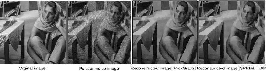
x∈Rn |aTx> b . As a stylized application, consider the low-light imaging problem in signal processing (Harmany et al., 2012), where the imag-ing data is collected by countimag-ing photons hittimag-ing a detector over the time. In this settimag-ing, we wish to accurately reconstruct an image in low-light, which leads to noisy measurements due to low photon count levels. We can express our observation model using the Poisson distribution as
P(y|A(x)) =
m
Y
i=1
(aTi x)yi yi!
e−aTix,
where x is the true image, A is a linear operator that projects the scene onto the set of observations, ai is thei-th row ofA, and y∈Zm+ is a vector of observed photon counts.
Via the log-likelihood formulation, we stumble upon a composite minimization problem:
x∗ := arg min x∈Rn
nXm
i=1
aTi x−
m
X
i=1
yilog(aTi x)
| {z }
=:f(x)
+g(x)o, (3)
where f(x) is self-concordant (but not standard). In the above formulation, the typical image priors g(x) include the `1-norm for sparsity in a known basis, total variation
semi-norm of the image, and the positivity of the image pixels. While the formulation (3) seems specific to imaging, it is also common in sparse regression with unknown noise variance (St¨adler et al., 2012), heteroscedastic LASSO (Dalalyan et al., 2013), barrier approximations of, e.g., the Dantzig selector (Candes and Tao, 2007) and quantum tomography (Banaszek et al., 1999) as well.
The current state of the art solver is called SPIRAL-TAP (Harmany et al., 2012), which biases the logarithmic term (i.e., log(aTi x+ε)→ log(aTi x), where ε1) and then applies non-monotone composite gradient descent algorithms for FL with a Barzilai-Borwein
step-size as well as other line-search strategies.
Logarithm of concave quadratic functions: The function f(x) :=−log σ2−kAx−yk2 2
is self-concordant with dom(f) :=
we consider the basis pursuit denoising (BPDN) formulation (van den Berg and Friedlander, 2008) as
x∗:= arg min x∈Rn
n
g(x) | kAx−yk22 ≤σ2o. (4) The BPDN criteria is commonly used in magnetic resonance imaging (MRI) where A is a subsampled Fourier operator,yis the MRI scan data, andσ2 is a known machine noise level
(i.e., obtained during a pre-scan). In (4), g is an image prior, e.g., similar to the Poisson imaging problem. Approximate solutions to (4) can be obtained via a barrier formulation
x∗t := arg min x∈Rn
n
−tlogσ2− kAx−yk22
| {z }
=:f(x)
+ g(x)o, (5)
where t >0 is a penalty parameter which controls the quality of the approximation. The BPDN formulation is quite generic and has several other applications in statistical regres-sion, geophysics, and signal processing.
Several different approaches solve the BPDN problem (4), some of which require pro-jections onto the constraint set, including Douglas-Rachford splitting, proximal methods, and the SPGL1 method (van den Berg and Friedlander, 2008; Combettes and Wajs, 2005).
1.2 Related Work
Our attempt is to briefly describe the work that revolves around (1) with the main as-sumptions of f ∈ FL and the proximal operator of g being computationally tractable.
In fact, Douglas-Rachford splitting methods can obtain numerical solutions to (1) when the self-concordant functions are endowed with tractable proximal maps. However, it is computationally easier to calculate the gradient off ∈ F2 than their proximal maps.
One of the main approaches in this setting is based on operator splitting. By presenting the optimality condition of problem (1) as an inclusion of two monotone operators, one can apply splitting techniques, such as forward-backward or Douglas-Rachford methods, to solve the resulting monotone inclusion (Briceno-Arias and Combettes, 2011; Facchinei and Pang, 2003; Goldstein and Osher, 2009). In our context, several variants of this approach have been studied. For example, projected gradient or proximal-gradient methods and fast proximal-gradient methods have been considered, see, e.g., (Beck and Teboulle, 2009a; Mine and Fukushima, 1981; Nesterov, 2007). In all these methods, the main assumption required to prove the convergence is the global Lipschitz continuity of the gradient of the smooth functionf. Unfortunately, whenf /∈ FL butf ∈ F2, these theoretical results on the global
convergence and the global convergence rates are no longer applicable.
the convex optimization context. Hence, it is unclear if this line of work is likely to lead to any rigorous guarantees whenf ∈ F2.
An emerging direction for solving composite minimization problems (1) is based on the proximal-Newton method. The origins of this method can be traced back to the work of (Bonnans, 1994), which relies on the concept ofstrong regularity introduced by (Robinson, 1980) for generalized equations. In the convex case, this method has been studied by several authors such as (Becker and Fadili, 2012; Lee et al., 2012; Schmidt et al., 2011). So far, methods along this line are applied to solve a generic problem of the form (1) even whenf ∈ F2. The convergence analysis of these methods is encouraged by standard Newton
methods and requires the strong regularity of the Hessian off near the optimal solution (i.e.,
µI ∇2f(x) LI). This assumption used in (Lee et al., 2012) is stronger than assuming
∇2f(x∗) to be positive definite at the solution x∗ as in our approach below. Moreover, the global convergence can only be proved by applying a certain globalization strategy such as line-search (Lee et al., 2012) or trust-region. Unfortunately, none of these assumptions can be verified before the algorithm execution for the intended applications. By exploiting the self-concordance concept, we can show the global convergence of proximal-Newton methods without any globalization strategy (e.g., line search or trust-region approach).
1.3 Our Contributions
Interior point methods are always an option while solving the self-concordant composite problems (1) numerically by means of disciplined convex programming (Grant et al., 2006; L¨ofberg, 2004). More concretely, in the IPM setting, we set up an equivalent problem to (1) that typically avoids the non-smooth term g(x) in the objective by lifting the problem dimensions with slack variables and introducing additional constraints. The new constraints may then be embedded into the objective through a barrier function. We then solve a sequence of smooth problems (e.g., with Newton methods) and “path-follow”3 to obtain
an accurate solution (Nemirovskii and Todd, 2008; Nesterov, 2004). In this loop, many of the underlying structures within the original problem, such as sparsity, can be lost due to pre-conditioning or Newton direction scaling (e.g., Nesterov-Todd scaling, Nesterov and Todd 1997). The efficiency and the memory bottlenecks of the overall scheme then heavily depends on the workhorse algorithm that solves the smooth problems.
In stark contrast, we introduce an algorithmic framework that directly handles the composite minimization problem (1) without increasing the original problem dimensions. For problems of larger dimensions, this is the main argument in favor of our approach. Instead of solving a sequence of smooth problems, we solve a sequence of non-smooth proximal problems with a variable metric (i.e., our workhorse). Fortunately, these proximal problems feature the composite form (1) with a Lipschitz gradient (and oft-times strongly convex) smooth term. Hence, we leverage the tremendous amount of research (cf., Table 1) done over the last decades. Surprisingly, we can even retain the original problem structures that lead to computational ease in many cases (e.g., see Section 4.1).
Our specific contributions can be summarized as follows:
1. We develop a variable metric framework for minimizing the sum f +g of a self-concordant function f and a convex, possibly nonsmooth function g. Our approach
relies on the solution of a convex subproblem obtained by linearizing and regularizing the first term f. To achieve monotonic descent, we develop a new set of analytic step-size selection and correction procedures based on the structure of the problem.
2. We establish both the global and the local convergence of different variable metric strategies. We first derive an expected result: when the variable metric is the Hes-sian ∇2f(xk) of f at iteration k, the resulting algorithm locally exhibits quadratic
convergence rate within an explicit region. We then show that variable metrics sat-isfying the Dennis-Mor´e-type condition (Dennis and Mor´e, 1974) exhibit superlinear convergence.
3. We pay particular attention to diagonal variable metrics as many of the proximal subproblems can be solved exactly (i.e., in closed form). We derive conditions on when these variants achieve locally linear convergence.
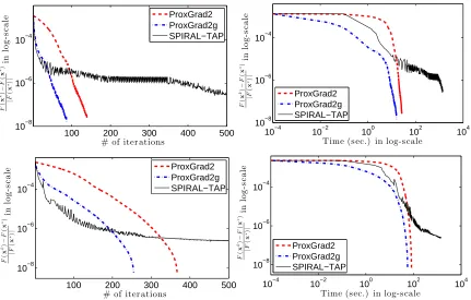
4. We apply our algorithms to the aforementioned real-world and synthetic problems to highlight the strengths and the weaknesses of our scheme. For instance, in the graph learning problem (2), our framework can avoid matrix inversions as well as Cholesky decompositions in learning graphs. In Poisson intensity reconstruction (3), up to around 80× acceleration is possible over the state-of-the-art solver.
We highlight three key practical contributions to numerical optimization. First, in the proximal-Newton method, our analytical step-size procedures allow us to do away with any globalization strategy (e.g., line-search). This has a significant practical impact when the evaluation of the functions is expensive. We show how to combine the analytical step-size selection with the standard backtracking or forward line-search procedures to enhance the global convergence of our method. Our analytical quadratic convergence characterization helps us adaptively switch fromdampedstep-size to afullstep-size. Second, in the proximal-gradient method setting, we establish a step-size selection and correction mechanism. The step-size selection procedure can be considered as a predictor, where existing step-size rules that leverage local information can be used. The step-size corrector then adapts the local information of the function to achieve the best theoretical decrease in the objective function. While our procedure does not require any function evaluations, we can further enhance convergence whenever we are allowed function evaluations. Finally, our framework, as we demonstrate in (Tran-Dinh et al., 2014a), accommodates a path-following strategy, which enable us to approximately solve constrained non-smooth convex minimization problems with rigorous guarantees.
2. Preliminaries
Notation: We reserve lower-case and bold lower-case letters for scalar and vector represen-tation, respectively. Upper-case bold letters denote matrices. We denote Sp+ (reps., S
p
++)
for the set of symmetric positive definite (reps., positive semidefinite) matrices of sizep×p. For a proper, lower semicontinuous convex functionf fromRn toR∪ {+∞}, we denote its domain by dom(f), i.e., dom(f) :={x∈Rn |f(x)<+∞}(see, e.g., Rockafellar 1970).
Weighted norm and local norm: Given a matrix H ∈ Sn++, we define the weighted
norm kxkH := √xTHx, ∀x∈
Rn; its dual norm is defined as kxk∗H := maxkykH≤1yTx=
√
xTH−1x. If H is only positive semidefinite (i.e., H ∈ Sn
+), then kxkH reduces to a semi-norm. Let f ∈ F2 and x ∈ dom(f) so that ∇2f(x) is positive definite. For a given
vectorv ∈Rn, the local norm aroundx∈dom(f) with respect tof is defined as kvkx := vT∇2f(x)v1/2, while the corresponding dual norm is given bykvk∗x= vT∇2f(x)−1v1/2
. Subdifferential and subgradient: Given a proper, lower semicontinuous convex function, we define the subdifferential ofg atx∈dom(g) as
∂g(x) :=
v∈Rn |g(y)−g(x)≥vT(y−x), ∀y∈dom(g) .
If∂g(x)6=∅then each element in∂g(x) is called a subgradient ofgatx. In particular, ifgis differentiable, we use ∇g(x) to denote its derivative at x∈dom(g), and∂g(x)≡ {∇f(x)}. Proximity operator: A basic tool to handle the nonsmoothness of a convex function g
is its proximity operator (or proximal operator) proxH
g , whose definition is given in Section
1. For notational convenience in our derivations, we alter this definition in the sequel as follows: Letg be a proper lower semicontinuous and convex in Rn and H∈Sn+. We define
PHg(u) := arg min x∈Rn
g(x) + (1/2)xTHx−uTx , ∀u∈Rn, (6)
as the proximity operator for the nonsmooth g, which has the following properties Hiriart-Urruty and Lemar´echal (2001).
Lemma 2 Assume that H ∈ Sn++. Then, the operator P
g
H in (6) is single-valued and
satisfies the following property:
(PHg(u)−PHg(v))T(u−v)≥
PHg(u)−PHg(v)
2
H, (7)
for all u,v∈Rn. Consequently,PHg is a nonexpansive mapping, i.e.,
P
g
H(u)−P
g
H(v)
H ≤ ku−vk ∗
H. (8)
Proof This lemma is already known in the literature, see, e.g., (Rockafellar, 1976). For the sake of completeness, we give a short proof here. The single-valuedness of PHg is ob-vious due to the strong convexity of the objective function in (6). Let ξu := PHg(u) and ξv:=PHg(v). By the definition of PHg, we have u−Hξu∈∂g(ξu) and v−Hξu ∈∂g(ξv). Since gis convex, we have (u−Hξu−(v−Hξv))T(ξu−ξv)≥0. This inequality leads to (u−v)T(ξ
u−ξv) ≥ (ξu−ξv)TH(ξu−ξv) = kξu−ξvk
2
Key self-concordant bounds: Based on (Nesterov, 2004, Theorems 4.1.7 and 4.1.8), for a given standard self-concordant function f, we recall the following inequalities
ω(ky−xkx) +∇f(x)T(y−x) +f(x)≤f(y), (9)
f(y)≤f(x) +∇f(x)T(y−x) +ω
∗(ky−xkx), (10) where ω : R → R+ is defined as ω(t) := t−ln(1 +t) and ω∗ : [0,1] → R+ is defined
as ω∗(t) := −t−ln(1−t). These functions are both nonnegative, strictly convex and increasing. Hence, (9) holds for all x,y ∈ dom(f), and (10) holds for all x,y ∈ dom(f) such that ky−xkx < 1. In contrast to the “global” inequalities for the function classes
FL and Fµ (cf., Figure 1), the self-concordant inequalities are based on “local” quantities.
Moreover, these bounds are no longer quadratic which prevents naive applications of the methods from FL,µ.
Remark 3 The proof of (9)-(10)is based on the condition∇2f(x)0 for allx∈dom(f), see (Nesterov, 2004). In this paper, we work with the functionf defined byf(x) :=ϕ(Ax+ b), where ϕ is a standard self-concordant function such that ∇2ϕ(u) 0 for all u ∈ dom(ϕ). Therefore, we have ∇2f(x) = AT∇2ϕ(Ax +b)A, which is possibly singular without further conditions on matrix A. Consequently, the local norm k · kx defined via
∇2f(x)reduces to a semi-norm. However, the inequalities (9)-(10)still hold w.r.t. this semi-norm. Indeed, sinceϕ is standard self-concordant with ∇2ϕ(u)0 for allu∈dom(ϕ), we haveϕ(ˆu)≥ϕ(u) +∇ϕ(u)T(ˆu−u) +ω kuˆ−uk
u
. By substitutingu=Ax+b∈dom(ϕ) and uˆ =Axˆ+b ∈dom(ϕ), (x,xˆ ∈dom(f)) into this inequality we obtain f(ˆx)≥f(x) +
∇f(x)T(ˆx−x) +ω(kxˆ−xk
x), which is indeed (9). The inequality (10)is proved similarly.
3. Composite Self-Concordant Optimization
In this section, we propose avariable metricoptimization framework that rigorously trades off computation and accuracy of solutions without transforming (1) into a higher dimension smooth convex optimization problem. We assume theoretically that the proximal subprob-lems can be solved exactly. However, our theory can be analyze for the inexact case, when we solve these problems up to a sufficiently high accuracy (typically, it is at least higher than (e.g., 0.1ε) the desired accuracy ε of (1) at the few last iterations), see, e.g., (Tran-Dinh et al., 2013b, 2014a). In our theoretical characterizations, we only rely on the following assumption:
Assumption A.1 The function f is convex and standard self-concordant (see Definition 1). The functiong:Rn→R∪ {+∞}is proper, closed and convex.
Under AssumptionA.1, we have dom(F) = dom(f)∩dom(g).
Unique solvability of (1) and its optimality condition: First, we show that problem (1) is uniquely solvable. The proof of this lemma can be done similarly as (Nesterov, 2004, Theorem 4.1.11) and is provided in Appendix A.1.
Lemma 4 Suppose that the functions f and g of problem (1) satisfy Assumption A.1. If λ(x) :=k∇f(x) +vk∗x < 1, for some x ∈ dom(F) and v ∈ ∂g(x) such that ∇2f(x) 0,
Since this problem is convex, the following optimality condition is necessary and sufficient:
0∈ ∇f(x∗) +∂g(x∗). (11)
The solutionx∗is calledstrongly regular if∇2f(x∗)0. In this case,∞> σ∗
max≥σ∗min>0,
whereσ∗min and σmax∗ are the smallest and the largest eigenvalue of∇2f(x∗), respectively.
Fixed-point characterization: Let H ∈ Sn+. We define SH(x) := Hx− ∇f(x). Then, from (11), we have
SH(x∗)≡Hx∗− ∇f(x∗)∈Hx∗+∂g(x∗).
By using the definition ofPHg(·) in (6), one can easily derive the fixed-point expression:
x∗=PHg (SH(x∗)), (12)
that is, x∗ is the fixed-point of the mapping RgH(·), where RHg (·) := PHg(SH(·)). The formula in (12) suggests that we can generate an iterative sequence based on the fixed-point principle, i.e., xk+1 := RgH(xk) starting from x0 ∈dom(F) for k≥0. Theoretically, under certain assumptions, one can ensure that the mapping RgH is contractive and the sequence generated by this scheme is convergent.
We note that if g ≡ 0 and H ∈ Sn++, then P
g
H defined by (6) reduces to P
g
H(·) = H−1(·). Consequently, the fixed-point formula (12) becomesx∗=x∗−H−1∇f(x∗), which is equivalent to∇f(x∗) = 0.
Our variable metric framework: Given a point xk ∈dom(F) and a symmetric positive semidefinite matrixHk, we consider the function
Q(x;xk,Hk) :=f(xk) +∇f(xk)T(x−xk) +
1 2(x−x
k)TH
k(x−xk), (13)
forx∈dom(F). The function Q(·;xk,Hk) is—seemingly—a quadratic approximation off
around xk. Now, we study the following scheme to generate a sequence
xk k≥0:
xk+1:=xk+αkdk, (14)
whereαk∈(0,1] is a step size and dk is a search direction.
Let sk be a solution of the following problem:
sk ∈ S(xk,Hk) := arg min
x∈dom(F)
n
Q(x;xk,Hk) +g(x)
o
=PHg k
Hkxk− ∇f(xk)
. (15)
Since we do not assume that Hk to be positive definite, the solution sk may not exist. We
require the following assumption:
Assumption A.2 The subproblem (15) has at least one solution sk, i.e., S(xk,Hk)6=∅.
In particular, ifHk∈Sn++, then the solutionskof (15) exists and is unique, i.e.,S(xk,Hk) =
Now, given sk, the directiondk is computed as
dk:=sk−xk. (16)
If we define Gk := Hkdk, then Gk is called the gradient mapping of (1) (Nesterov, 2004),
which behaves similarly as gradient vectors in non-composite minimization. Since problem (15) is solvable due to AssumptionA.2, we can write its optimality condition as
0∈ ∇f(xk) +Hk(sk−xk) +∂g(sk). (17)
It is easy to see that if dk = 0, i.e., sk ≡ xk, then (17) reduces to 0∈ ∇f(xk) +∂g(xk), which is exactly (11). Hence,xk is a solution of (1).
In the variable metric framework, depending on the choice of Hk, the iteration scheme
(14) leads to different methods for solving (1). For instance:
1. IfHk:=∇2f(xk), then the method (14) is aproximal-Newton method.
2. If Hk is a symmetric positive definite matrix approximation of ∇2f(xk), then the
method (14) is aproximal-quasi Newton method.
3. IfHk:=LkI, whereLkis, say, an approximation for the local Lipschitz constant off
and I is the identity matrix, then the method (14) is aproximal-gradient method.
Many of these above methods have been studied for (1) when f ∈ FL: cf., (Beck and
Teboulle, 2009a; Becker and Fadili, 2012; Chouzenoux et al., 2013; Lee et al., 2012). Note however that, since the self-concordant part f of F is not (necessarily) globally Lipschitz continuously differentiable, these approaches are generally not applicable in theory.
Given the search directiondkdefined by (16), we define the following proximal-Newton decrement4 λ
k and the weighted [semi-]norm βk
λk:=kdkkxk =
(dk)T∇2f(xk)dk1/2 andβ
k:=kdkkHk. (18)
In the sequel, we study three different instances of the variable metric strategy in detail. Since we do not assume∇2f(xk)0,λ
k= 0 may not implydk= 0.
Remark 5 If g ≡0 and ∇2f(xk) ∈
Sn++, then dk =−∇2f(xk)−1∇f(xk) is the standard Newton direction. In this case,λk defined by (18) reduces toλk ≡ k∇f(xk)k∗xk, the Newton decrement defined in (Nesterov, 2004, Chapter 4). Moreover, we have λk ≡ λ(xk), as
defined in Lemma 4.
3.1 A Proximal-Newton Method
If we choose Hk := ∇2f(xk), then the method described in (14) is called the proximal
Newton algorithm. For notational ease, we redefine skn := sk and dkn := dk, where the subscriptnis used to distinguish proximal Newton related quantities from the other variable
metric strategies. Moreover, we use the shorthand notation Px¯g := P∇g2f(¯x), whenever ¯x∈ dom(f). Using (15) and (16), skn and dknare given by
skn:=Pxgk
∇2f(xk)xk− ∇f(xk), dkn:=skn−xk. (19) Then, the proximal-Newton method generates a sequence
xk k≥0 starting from x0 ∈
dom(F) according to
xk+1 :=xk+αkdkn, (20)
where αk ∈ (0,1] is a step size. If αk < 1, then the iteration (20) is called the damped
proximal-Newton iteration. If αk= 1, then it is called the full-step proximal-Newton
itera-tion.
Global convergence: We first show that with an appropriate choice of the step-size
αk ∈(0,1], the iterative sequence
xk k≥0 generated by the damped-step proximal Newton scheme (20) is a decreasing sequence; i.e.,F(xk+1)≤F(xk)−ω(σ) wheneverλk ≥σ, where
σ > 0 is fixed. The following theorem provides an explicit formula for the step size αk
whose proof can be found in Appendix A.2.
Theorem 6 If αk:= (1 +λk)−1 ∈(0,1], then the scheme in (20) generates xk+1 satisfies
F(xk+1)≤F(xk)−ω(λk). (21)
Moreover, the step αk is optimal. The number of iterations to reach the point xk such that
λk< σ for some σ∈(0,1)is kmax:=
j
F(x0)−F(x∗)
ω(σ)
k
+ 1.
Local quadratic convergence rate: For anyx∈dom(f) such that∇2f(x)0, we define
the Dikin ellipsoid W0(x, r) as W0(x, r) :=
y ∈dom(f) :ky−xkx < r , see (Nesterov, 2004). We now establish the local quadratic convergence of the scheme (20). A complete proof of this theorem can be found in Appendix A.3.
Theorem 7 Suppose thatx∗ is the unique solution of (1)and is strongly regular. Suppose further that ∇2f(x)0 for allx∈ W0(x∗,1). Let
xk k≥0 be a sequence generated by the proximal Newton scheme (20) withαk∈(0,1]. Then:
a) If αkλk<1−√12, then it holds that
λk+1≤
1−αk+ (2α2k−αk)λk
1−4αkλk+ 2α2kλ2k
λk. (22)
b) If the sequence
xk k≥0 is generated by the damped proximal-Newton scheme (20), starting from x0 such that λ0 ≤¯σ :=
√
5−2≈0.236068 and αk:= (1 +λk)−1, then
{λk}k locally converges to0+ at a quadratic rate.
Consequently, the sequence
xk k≥0 also locally converges to x∗ at a quadratic rate in both cases b) and c), i.e., kxk−x∗kx∗
k≥0 locally converges to0
+ at a quadratic rate.
A two-phase algorithm for solving (1): Now, by the virtue of the above analysis, we can propose a two-phase proximal-Newton algorithm for solving (1). Initially, we perform the damped-step proximal-Newton iterations until we reach the quadratic convergence region (Phase 1). Then, we perform full-step proximal-Newton iterations, until we reach the desired accuracy (Phase 2). The pseudocode of the algorithm is presented in Algorithm 1.
Algorithm 1 (Proximal-Newton algorithm) Inputs: x0 ∈dom(F), tolerance ε >0.
Initialization: Select a constant σ∈(0,(5−
√
17)
4 ], e.g.,σ := 0.2.
for k= 0 toKmax do
1. Compute the proximal-Newton search directiondkn as in (19). 2. Compute λk:=
dkn
xk.
3. if λk > σthen xk+1:=xk+αkdkn, whereαk := (1 +λk)−1.
4. elseif λk > εthen xk+1 :=xk+dkn.
5. elseterminate. end for
The radius σ of the quadratic convergence region in Algorithm 1 can be fixed at any value in (0,σ¯], e.g., at its upper bound ¯σ. An upper bound Kmax of the iterations can also
be specified, if necessary. The computational bottleneck in Algorithm 1 is typically incurred Step 1 in Phase 1 and Phase 2, where we need to solve the subproblem (15) to obtain a search direction dkn. When problem (15) is strongly convex, i.e., ∇2f(xk)∈
Sn++, one can
apply first order methods to efficiently solve this problem with a linear convergence rate (see, e.g., Beck and Teboulle 2009a; Nesterov 2004, 2007) and make use of a warm-start strategy by employing the information of the previous iterations.
Remark 8 From Remark 3 we see that if∇f(xk)0, thenλk= 0 may not imply dk = 0. Therefore, we can add an auxiliary stopping criterion βk := kdkk2 ≤ ε to Algorithm 1 so that we can avoid the termination of Algorithm 1 at a non-optimal point xk.
Iteration-complexity analysis.The choice of σ in Algorithm 1 can trade-off the number of iterations between the damped-step and full-step iterations. If we fix σ = 0.2, then the complexity of the full-step Newton phase becomes O ln ln 0.ε28
. The following theorem summarizes the complexity of the proposed algorithm.
Theorem 9 The maximum number of iterations required in Algorithm 1 does not exceed Kmax :=
jF(x0)−F(x∗)
0.017
k
+
1.5 ln ln 0.28
ε
+ 2 provided that σ = 0.2 to obtain λk ≤ ε.
Consequently, kxk−x∗kx∗ ≤2ε, where x∗ is the unique solution of (1).
Proof Let σ = 0.2. From the estimate (22) of Theorem 7 and αk−1 = 1 we have λk ≤
(1−4λk−1 + 2λ2k−1)
−1λ2
that λk ≤(1−4σ+ 2σ2)−1λ2k−1 ≤cλ2k−1, where c := 3.57. This implies λk ≤c2
k−1 λ20k ≤ c2k−1σ2k. The stopping criterion λ
k ≤ ε in Algorithm 1 is ensured if (cσ)2
k
≤ cε. Since
cσ ≈ 0.71 < 1, the last condition leads to k ≥ (ln 2)−1ln−ln(cσ)
−ln(cε)
. By using c = 3.57,
σ= 0.2 and the fact that ln(2)−1 <1.5, we can show that the last requirement is fulfilled if k≥1.5 ln ln 0.28
ε
+ 1. Now, combining the last conclusion and Theorem 6 with noting thatω(σ)>0.017 we obtainKmax as in Theorem 9.
Finally, we provekxk−x∗kx∗ ≤2ε. Indeed, we haverk:=kxk−x∗kx∗ ≤ kx
k+1−xkk
xk 1−kxk−x∗k
x∗+
kxk+1−xkkx∗ = λk
1−rk +rk+1, whenever rk < 1. Next, using (84) with αk = 1, we have rk+1 ≤
(3−rk)r2
k 1−4rk+2r2
k
. Combining these inequalities, we obtain (1−rk)(1−7rk+3rk2)rk 1−4rk+2r2
k ≤
λk ≤ ε.
Since the function s(r) := (1−r1)(1−4−r+27r+3r2r2)r attains a maximum at r
∗ ≈ 0.08763 and it
is increasing on [0, r∗]. Moreover, (1−rk)(1−7rk+3r2k) 1−4rk+2r2
k ≥
0.5 for rk ∈ [0, r∗], which leas to
0.5rk ≤
(1−rk)(1−7rk+3rk2)rk 1−4rk+2rk2 ≤
ε. Hence,rk ≤2εprovided that rk ≤r0 ≤r∗ ≈0.08763.
Remark 10 When g ≡ 0, we can modify the proof of estimate (22) to obtain a tighter bound λk+1 ≤
λ2
k
(1−λk)2. This estimate is exactly (Nesterov, 2004), which implies that the radius of the quadratic convergence region is σ¯:= (3−√5)/2.
A modification of the proximal-Newton method: In Algorithm 1, if we remove Step 4 and replace analytic step-size selection calculation in Step 3 with a backtracking line-search, then we reach the proximal Newton method of (Lee et al., 2012). Hence, this approachin practice might lead to reduced overall computation since our step-sizeαk is selected optimally with
respect to the worst case problem structures as opposed to the particular instance of the problem. Since the backtracking approach always starts with the full-step, we also do not need to know whether we are within the quadratic convergence region. Moreover, the cost of evaluating the objective at the full-step in certain applications may not be significantly worse than the cost of calculating αk or may be dominated by the cost of calculating the
Newton direction.
In stark contrast to backtracking, our new theory behooves us to propose a new forward line-search procedure as illustrated by Figure 2. The idea is quite simple: we start with the
0 1
ppp ppp ppp ppp ppp
r u
α∗k
s R R
Enhanced backtracking
@ @ R
Standard backtracking
Forward line-search
Overjump
Figure 2: Illustration of step-size selection procedures.
“optimal” step-sizeαk and increase it towards full-step with a stopping condition based on
access to the side information on whether or not we are within the quadratic convergence region, and hence, we can automatically switch to Step 4 in Algorithm 1. Alternatively, calculation of the analytic step-size can enhance backtracking since the knowledge of αk
reduces the backtracking range from (0,1] to (αk,1] with the side-information as to when
to automatically take the full-step without function evaluation.
3.2 A Proximal Quasi-Newton Scheme
Even if the functionf is self-concordant, the numerical evaluation of∇2f(x) can be
expen-sive in many applications (e.g.,f(x) :=Pp
j=1fj(Ajx), withpn). Hence, it is interesting
to study proximal quasi-Newton method for solving (1). Our interest in the quasi-Newton methods in this paper is for completeness; we do not provide any algorithmic details or implementations on our quasi-Newton variant.
To this end, we need a symmetric positive definite matrixHkthat approximates∇2f(xk)
at the iterationk. As a result, our main assumption here is that matrix Hk+1 at the next
iterationk+ 1 satisfies the secant equation:
Hk+1(xk+1−xk) =∇f(xk+1)− ∇f(xk). (23)
For instance, it is well-known that the sequence of matrices {Hk}k≥0 updated by the
fol-lowing BFGS formula satisfies the secant equation (23) (Nocedal and Wright, 2006):
Hk+1 :=Hk+
1 (yk)Tzky
k(yk)T − 1
(zk)TH kzk
Hkzk(Hkzk)T, (24)
wherezk :=xk+1−xkand yk:=∇f(xk+1)− ∇f(xk). Other methods for updating matrix Hk can be found in (Nocedal and Wright, 2006), which are not listed here.
In this subsection, we only analyze the full-step proximal quasi-Newton scheme based on the BFGS updates. The global convergence characterization of the BFGS quasi-Newton method can be obtained using our analysis in the next subsection. To this end, we have the following update equation, where the subscript q is used to distinguish the quasi-Newton method:
xk+1:=xk+dkq. (25)
Here we usedkq to stand for the proximal quasi-Newton search direction. Under certain assumptions, one can prove that the sequence
xk k≥0 generated by (25) converges tox∗ the unique solution of (1). One of the common assumptions used in quasi-Newton methods is the Dennis-Mor´e condition, see (Dennis and Mor´e, 1974). Adopting the Dennis-Mor´e criterion, we impose the following condition in our context:
lim
k→∞
Hk− ∇2f(x∗)
(xk+1−xk)
∗ x∗
kxk+1−xkk
x∗
= 0. (26)
The Dennis-Mor´e condition becomes standard in smooth optimization. Examples can be found, e.g., in (Byrd and Nocedal, 1989; Nocedal and Wright, 2006). Now, we establish the superlinear convergence of the sequence
Theorem 11 Assume that x∗ is the unique solution of (1) and is strongly regular. Let matrix Hk maintains the secant equation (23) and let
xk k≥0 be a sequence generated by scheme (25). Then the following statements hold:
(a) Suppose, in addition, that the sequence of matrices{Hk}k≥0 satisfies the Dennis-Mor´e condition (26) for sufficiently large k. Then the sequence xk k≥0 converges to the solution x∗ of (1) at a superlinear rate provided that x0−x∗
x∗ <1.
(b) Suppose that a matrix H0 0 is chosen. Then (yk)Tzk >0 for all k≥0 and hence the sequence{Hk}k≥0 generated by(24)is symmetric positive definite and satisfies the secant equation (23). Moreover, if the sequence xk k≥0 generated by (25) satisfies
P∞
k=0
xk−x∗
x∗ <+∞, then this sequence converges tox
∗ at a superlinear rate.
The proof of this theorem can be found in Appendix A.3. We note that if the sequence
xk k≥0locally converges tox∗at a linear rate w.r.t. the local norm atx∗, i.e.
xk+1−x∗
x∗ ≤
κxk−x∗
x∗ for someκ ∈(0,1) andk≥0, then the condition
P∞
k=0
xk−x∗
x∗ <+∞ automatically holds. From (26) we also observe that the matrix Hk is required to well
approximate ∇2f(x∗) along the direction dk
q, which is not in the whole space.
3.3 A Proximal-Gradient Method
If we choose matrixHk := Dk, where Dk is a positive diagonal matrix, then the iterative
scheme (14) is called the proximal-gradient scheme. In this case, we can write (14) as
xk+1:=xk+αkdkg = (1−αk)xk+αkskg, (27)
where αk ∈ (0,1] is an appropriate step size, dkg is the proximal-gradient search direction
and skg ≡sk as in (15).
The following lemma shows how we can choose the step size αk corresponding to Dk
such that we obtain a descent direction in the proximal-gradient scheme (27). The proof of this lemma can be found in Appendix A.2.
Lemma 12 Letxk k≥0 be a sequence generated by (27). Suppose that the matrix Dk 0
is chosen such that the step size αk satisfies αk := β2
k
λk(λk+β2
k) ∈
(0,1] (see below), where
βk := kdkgkDk and λk := kd
k
gkxk. Then
xk k≥0 ⊂ dom(F) and the following estimate holds
F(xk+1)≤F(xk)−ω βk2/λk
, (28)
where ω(τ) :=τ −ln(1 +τ)≥0.
From Lemma 12, we observe that αk ≤1 if λ2
k
β2
k
+λk ≥ 1. It is obvious that ifλk ≥ 1
then the last condition is automatically satisfied. We only consider the caseλk<1. In fact,
sinceλk≥0, we relax actually the condition λ2
k
β2
k
Algorithm 2 (Proximal-gradient method) Inputs: x0 ∈dom(F), tolerance ε >0. for k= 0 tokmax do
1. Choose an appropriate Dk0 based on (30).
2. Compute dkg :=PDg
k Dkx
k− ∇f(xk)
−xk due to (15). 3. Compute βk:=kdkgkDk and λk:=kd
k gkxk.
4. Ifek:=kdkgk2 ≤εthen terminate.
5. Updatexk+1:=xk+α
kdkg, whereαk:= β2
k
λk(λk+βk2) ∈
(0,1]. end for
We now study the case Dk:=LkI, whereLk ≥L >0 is a positive constant andIis the identity matrix with dimensions apparent from the context. Hence,βk2 =Lkkdkgk22 and
λ2k βk2 =
(dkg)T∇2f(xk)dk g
Lkkdkgk22 .
However, since
σmin(∇2f(xk))≤σk:=
(dkg)T∇2f(xk)dk g
kdk gk22
≤σmax(∇2f(xk)), (29)
the conditionλk≥βk is equivalent to
Lk≤σk, (30)
where σkmin := σmin(∇2f(xk)) and σkmax := σmax(∇2f(xk)) are the smallest and largest
eigenvalue of∇2f(xk), respectively. Under the assumption that dom(f) contains no
straight-line, then we have the Hessian ∇2f(xk) 0 by (Nesterov, 2004, Theorem 4.1.3), which
implies that σkmin > 0. Therefore, in the worst-case, we can choose Lk := σmink . However,
this lower bound may be too conservative. In practice, we can apply abisection procedure to meet the condition (30). It is not difficult to prove via contradiction that the number of bisection steps is upper bounded by a constant.
We note that if g is separable, i.e.,g(x) := Pn
i=1gi(xi) (e.g., g(x) :=ρkxk1), then we
can computeskD
k in (15) in a component-wise fashion as
(skLk)i:=Pτgki i
xki −τik(∇f(xk))i
, i= 1, . . . , n, (31)
where τik := 1/(Dk)ii and Pτgii(·) is the proximity operator of gi function, with parameter τi. The computation of λk only requires one matrix-vector multiplication and one vector
inner-product; but it can be reduced by exploiting concrete structure of the smooth partf. Based on Lemma 12, we describe the proximal-gradient scheme (27) in Algorithm 2. The main computation cost of Algorithm 2 is incurred at Step 2 and in calculating λk. If
step of Algorithm 2 is Step 2, which depends on the cost of prox-operatorPDg
k. In practice,
Dk is determined by a bisection procedure whenever λk < 1, which requires additional
computational cost. If we choose Dk:=LkI, then in order to fulfill (30), we can perform a back-tracking line search procedure on Lk. This line search procedure does not require the
evaluations of the objective function. We modify Steps 1-3 of Algorithm 2 as
1. Initialize Lk:=L0k>0, e.g., by a Barzilai-Borwein step.
2. Compute dk g :=P
g
LkIk Lkx
k− ∇f(xk)
−xk due to (15).
3a. Computeβk:=kdkgkLkI and λk:=kd
k gkxk.
3b. Ifλ2k/βk2+λk <1, then setLk:=Lk/2 and go back to Step 2.
We note that computing λk at Step 3 does not need to form the full Hessian ∇2f(xk), it
only requires a directional derivative, which is relatively cheap in applications (Nocedal and Wright, 2006, Chapter 7).
Global and local convergence. The global and local convergence of Algorithm 2 is stated in the following theorems, whose proof can be found in Appendix A.2.
Theorem 13 Assume that there existsL >0such thatDkLIfork≥0, and the solution x∗ of (1)is unique. Let the sublevel set
LF(F(x0)) :=
x∈dom(F) |F(x)≤F(x0)
be bounded. Then, the sequencexk k≥0, generated by Algorithm 2, converges to the unique solution x∗ of (1).
Theorem 14 Assume that x∗ is the unique solution of (1) and is strongly regular. Let
xk k≥0 be the sequence generated by Algorithm 2. Then, for ksufficiently large, if
[Dk− ∇2f(x∗)]dkg
∗ x∗
kdk
gkx∗ < 1
2, (32)
then
xk k≥0 locally converges to x∗ at a linear rate. In particular, if Dk := LkI and
γ∗ := max
n
1−
Lk
σ∗min
,
1−
Lk
σ∗ max
o
< 12, then the condition (32) holds.
We note that x∗ is unknown; thus, evaluating γ∗ a priori is infeasible in reality. In implementation, one can choose an appropriate value Lk ≥ L > 0 and then adaptively
updateLkbased on the knowledge of the eigenvalues of∇2f(xk) near to the solutionx∗. The
condition (32) can be expressed as (dkg)T[L2
k∇2f(x
∗)−1+∇2f(x∗)
−2LkI]dkg ≤(1/4)kdkgk2x∗, which leads to
(3/4)kdkgk2x∗+L2[kdgkk∗x∗]2<2Lkkdkgk22. (33) We note that to find Lk such that (33) holds, we require kdkgkx∗∗kdkgkx∗ <
q
4
3kdkgk22. If
last condition in Theorem 14 seems too imposing, we claim that, for most f and g, we only require (33) to be satisfied (see also the empirical evidence in Subsection 5.2.1). The condition (32) (or (33)) can be referred to as arestrictedapproximation gap between Dk
and the true Hessian∇2f(x∗) along the direction dk
g fork sufficiently large. For instance,
when g is based on the `1-norm/the nuclear norm, the search direction dkg have at most
twice the sparsity/rank of x∗ near the convergence region.
Remark 15 From the scheme (27) we observe that the step size αk <1 may not preserve
some of the desiderata on xk+1 due to the closed form solution of the prox-operator PDg k. For instance, when g is based on the `1-norm, αk <1, might increase the sparsity level of
the solution as opposed to monotonically increasing it. However, in practice, the numerical values of αk are often 1 near the convergence, which maintain properties, such as sparsity,
low-rankedness, etc.
Global convergence rate: In proximal gradient methods, proving global convergence rate guarantees requires a global constant to be knowna priori—such as the Lipschitz constant. However such an assumption does not apply for the class of just self-concordant functions that we consider in this paper. We only characterize the following property in an ergodic sense. Let
xk k≥0 be the sequence generated by (2). We define
¯
xk:=Sk−1
k
X
j=0
αjxj, where Sk:= k
X
j=0
αj >0. (34)
Then we can show thatF(¯xk)−F∗≤ L¯k 2Sk
x0−x∗
2
2, where ¯Lk:= max0≤j≤kLj. Ifαj ≥α >0
for 0≤j ≤k, then Sk ≥α(k+ 1), which leads to F(¯xk)−F∗ ≤
¯
Lk 2(k+1)α
x0−x∗
2 2. The
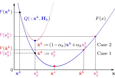
proof of this statement can be found in (Tran-Dinh et al., 2014b), which we omit here. A modification of the proximal-gradient method: If the pointskggenerated by (15) belongs to dom(F), then F(skg)<+∞. Similarly to the definition of xk+1 in (27), we can define a new trial point:
ˆ
xk:= (1−αk)xk+αkskg. (35)
IfF(sk
g)≤F(xk), then, by the convexity ofF, it is easy to show that:
F(ˆxk) =F (1−αk)xk+αkskg
≤(1−αk)F(xk) +αkF(skg)
F(skg)≤F(xk)
≤ F(xk).
In this case, based on the function valuesF(skg),F(ˆxk) andF(xk) we can eventually choose the next iterationxk+1 as follows:
xk+1 :=
skg ifsk∈dom(F) and F(skg)< F(ˆxk) (Case 1),
ˆ
xk otherwise (Case 2). (36)
The idea of this greedy modification is illustrated in Figure 3. We note that here we need to check skg ∈dom(F) such that F(sgk)< F(xk) and additional function evaluationsF(skg) and F(ˆxk). However, careful implementations can recycle quantities that enable us to evaluate the objective atskg and atxk+1 with very little overhead over the calculation ofαk
-6r
r
r
r
r
r
0
x∗
xk sk
g xˆk skg x
F(xk)
F(skg)
F(sk
g)
F(ˆxk)
F(x)
Q(·;xk,H
k)
ˆ
xk:= (1−αk)xk+α
kskg ˆ
xk:=sk
g Case 1
Case 2
Figure 3: Illustration of the modified proximal-gradient method
4. Concrete Instances of our Optimization Framework
We illustrate three instances of our framework for some of the applications described in Section 1. For concreteness, we describe only the first and second order methods. Quasi-Newton methods based on (L-)BFGS updates or other adaptive variable metrics can be similarly derived in a straightforward fashion.
4.1 Graphical Model Selection
We customize our optimization framework to solve the graph selection problem (2). For notational convenience, we maintain a matrix variable Θ instead of vectorizing it. We observe thatf(Θ) :=−log(det(Θ)) + tr( ˆΣΘ) is a standard self-concordant function, while
g(Θ) :=ρkvec(Θ)k1 is convex and nonsmooth. The gradient and the Hessian of f can be computed explicitly as∇f(Θ) := ˆΣ−Θ−1 and∇2f(Θ) :=Θ−1⊗Θ−1, respectively. Next,
we formulate our proposed framework to construct two algorithmic variants for (2).
4.1.1 Dual Proximal-Newton Algorithm
We consider a second order algorithm via a dual solution approach for (15). This approach is first introduced in our earlier work (Tran-Dinh et al., 2013a), which did not consider the new modifications we propose in Section 3.1.
We begin by deriving the following dual formulation of the convex subproblem (15). Let pk :=∇f(xk), the convex subproblem (15) can then be written equivalently as
min x∈Rn
n
(1/2)xTHkx+ (pk−Hkxk)Tx+g(x)
o
. (37)
By using the min-max principle, we can write (37) as
max u∈Rnx∈min
Rn
n
(1/2)xTHkx+ (pk−Hkxk)Tx+uTx−g∗(u)
o
, (38)
where g∗ is the Fenchel conjugate function of g, i.e., g∗(u) := sup x
uTx−g(x) . Solving the inner minimization in (38) we obtain
min u∈Rn
where ˜pk:=H−k1pk−xk. Note that the objective functionϕ(u) :=g∗(u) + (1/2)uTH−k1u+
˜
pTku of (39) is strongly convex, one can apply the fast projected gradient methods with a linear convergence rate for solving this problem, see (Nesterov, 2007; Beck and Teboulle, 2009a).
In order to recover the solution of the primal subproblem (15), we note that the solution of the parametric minimization problem in (38) is given byx∗(u) :=xk−H−k1(pk+u). Let
u∗xk be the optimal solution of (39). We can recover the primal proximal-Newton search
directiondk defined in (16) as
dkn=−∇2f(xk)−1 ∇f(xk) +u∗ xk
. (40)
To compute the quantityλk defined by (18) in Algorithm 1, we use (40) such that:
λk=kdknkxk =k∇f(xk) +u∗xkk
∗
xk. (41)
Note that computing λk by (41) requires the inverse of the Hessian matrix∇2f(xk).
Surprisingly, this dual approach allows us to avoid matrix inversion as well as Cholesky decomposition in computing the gradient ∇f(Θi) and the Hessian ∇2f(Θi) of f in graph
selection. An alternative is of course to solve (15) in its primal form. Though, in such case, we need to compute Θ−i 1 at each iterationi(say, via Cholesky decompositions).
The dual subproblem (39) becomes as
U∗= arg min kvec(U)k∞≤1
n
(1/2)tr((ΘiU)2) + tr(QUe ) o
, (42)
for the graph selection, whereQe :=ρ−1[ΘiΣΘb i−2Θi]. Given the dual solutionU∗of (42),
the primal proximal-Newton search direction (i.e. the solution of (15)) is computed as
∆i :=− (ΘiΣb −I)Θi+ρΘiU∗Θi
. (43)
The quantityλi defined in (41) can be computed as follows, where Wi :=Θi(Σb +ρU∗):
λi:= p−2·tr (Wi) + tr Wi2
1/2
. (44)
Algorithm 3 summarizes the description above. Overall, this proximNewton (PN) al-gorithm does not require any matrix inversions or Cholesky decompositions. It only needs matrix-vector and matrix-matrix calculations, which might be attractive for different com-putational platforms (such as GPUs or simple parallel implementations). Note however that as we work through the dual problem, the primal solution can be dense even if majority of the entries are rather small (e.g., smaller than 10−6).5
We now explain the underlying costs of each step in Algorithm 3, which is useful when we consider different strategies for the selection of the step sizeαk. The computation ofQe
and∆irequire basic matrix multiplications. For the computation ofλi, we require two trace
operations: tr(Wi) inO(p) time-complexity and tr(W2i) inO(p2) complexity. We note here
Algorithm 3 (Dual PN for graph selection (DPNGS))
Input: Matrix Σb 0 and a given tolerance ε >0. Set σ:= 0.25(5−
√
17). Initialization: Find a starting pointΘ00.
for i= 0 toimaxdo 1. SetQe :=ρ−1
ΘiΣΘb i−2Θi
. 2. Compute U∗ in (42).
3. Compute λi by (44), whereWi:=Θi(Σb+ρU∗).
4. Ifλi≤εterminate.
5. Compute ∆i:=−
(ΘiΣb −I)Θi+ρΘiU∗Θi
.
6. Ifλi> σ, then set αi:= (1 +λi)−1. Otherwise, setαi = 1.
7. UpdateΘi+1:=Θi+αi∆i.
end for
that, while Wi is a dense matrix, the trace operation in the latter case requires only the
computation of the diagonal elements ofWi2. GivenΘi,αiand ∆i, the calculation ofΘi+1
has O(p2) complexity. In contrast, evaluation of the objective can be achieved through Cholesky decompositions, which has O(p3) time complexity.
To compute (42), we can use the fast proximal-gradient method (FPGM) (Nesterov, 2007; Beck and Teboulle, 2009a) with step size 1/LwhereLis the Lipschitz constant of the gradient of the objective function in (42). It is easy to observe that L:= γmax2 (Θi) where
γmax(Θi) is the largest eigenvalue of Θi. For sparse Θi, we can approximately compute
γmax(Θi) is O(p2) by using iterative power methods (typically, 10 iterations suffice). The
projection onto kvec(U)k∞ ≤1 clips the elements by unity in O(p2) time. Since FPGM requires a constant number of iterationskmax (independent of p) to achieve anεin solution
accuracy, the time-complexity for the solution in (42) isO(kmaxM), whereM is the cost of
matrix multiplication. We have also implemented block coordinate descent and active set methods which scaleO(p2) in practice when the solution is quite sparse.
Overall, the major operation with general proximal maps in the algorithm is typically the matrix-matrix multiplications of the form ΘiUΘi, where Θi and U are symmetric
positive definite. This operation can naturally be computed (e.g., in a GPU) in a parallel or distributed manner. For more details of such computations we refer the reader to (Bertsekas and Tsitsiklis, 1989). It is important to note that without Cholesky decompositions used in objective evaluations, the basic DPNGS approach theoretically scales with the cost of matrix-matrix multiplications.
4.1.2 Proximal-Gradient Algorithm
Since g(Θ) :=ρkvec(Θ)k1 and ∇f(Θi) =vec(Σb −Θ−i 1), the subproblem (15) becomes:
∆i+1:=Tτiρ Θi−τi(Σb −Θ−i 1)
−Θi, (45)
where Tτ : Rp×p → Rp×p is the component-wise matrix thresholding operator which is defined asTτ(Θ) := max{0,|Θ| −τ}. We also note that the computation of∆i+1requires a
matrix inversionΘ−i 1. SinceΘi is positive definite, one can apply Cholesky decompositions
Θ−i 1∆i
2. We also chooseLi := 0.5k∇ 2f(Θ
i)k2= 0.5kΘ−i 1k22. The above are summarized
in Algorithm 4.
Algorithm 4 (Proximal-gradient method for graph selection (ProxGrad1)) Initialization: Choose a starting pointΘ00 .
for i= 0 toimaxdo
1. Compute Θ−i 1 via Cholesky decomposition. 2. Choose Li satisfying (30) and setτi :=L−i 1.
3. Compute the search direction∆i as (45).
4. Compute βi :=Likvec(∆i)k2 and λi:=kΘ−i 1∆ik2.
5. Determine the step sizeαi:= λi(λβi+i βi).
6. UpdateΘi+1:=Θi+αi∆i.
end for
The per iteration complexity is dominated by matrix-matrix multiplications and Cholesky decompositions for matrix inversion calculations. In particular, Step 1 requires a Cholesky decomposition with O(p3) time-complexity. Step 2 requires to compute `2-norm of a sym-metric positive matrix, which can be done by a power-method in O(p2) time-complexity. The complexity of Steps 3, 4 and 6 requiresO(p2) operations. Step 2 may require additional bisection steps as mentioned in Algorithm 2 wheneverλk<1.
4.2 Poisson Intensity Reconstruction
We now describe a variant of Algorithm 2; a similar instance based on Algorithm 1 can be easily devised and we omit the details here. First, we can easily check that the function
˜
f(x) := Pm
i=1 aTi x−yilog(aTi x)
in (3) is convex and self-concordant with parameter
Mf˜:= 2·max
n
1
√
yi |yi>0, i= 1, . . . , m
o
, see (Nesterov, 2004, Theorem 4.1.1). We define the functions f and g as
f(x) :=
M2˜
f
4 f˜(x), g(x) :=
M2˜
f
4 ρφ(x) +δ{u |u≥0}(x)
, (46)
wheref andgsatisfy Assumption 1 andδC is the indicator function ofC. Thus, the problem in (3) can be equivalently transformed into (1). Here, the gradient and the Hessian of f
satisfy:
∇f(x) =
M2˜
f
4
m
X
i=1
1− yi
aTix
ai and ∇2f(x) =
M2˜
f
4
m
X
i=1 yi
(aTi x)2aia
T
i, (47)
respectively. For a given vectord∈Rn, the local normkdkx can then be written as
kdkx:= dT∇2f(x)d
1/2
= Mf˜ 2
m
X
i=1
yi(aTi d)2
(aTi x)2
!1/2
. (48)
For the Poisson model, the subproblem (15) is expressed as follows:
min x≥0
n
(1/2)kx−wkk22+ρkφ(x)
o
, (49)
where wk := xk −Lk−1∇f(xk) and ρk := ρM2
˜
f
4Lk. As a penalty function φ in the Poisson
intensity reconstruction, we use the Total Variation norm (TV-norm), defined as φ(x) :=
kDxk1 (isotropic) orφ(x) :=kDxk1,2 (anti-isotropic), whereDis a forward linear operator
(Chambolle and Pock, 2011; Beck and Teboulle, 2009b). For both TV-norm regularizers, the method proposed in (Beck and Teboulle, 2009b) can solve (49) efficiently.
The above discussion leads to Algorithm 5. We note that the constant Lk at Step 2 of
this algorithm can be estimated based on different rules. In our implementation below, we initializeLkat a Barzilai-Borwein step size, i.e.,Lk:= (∇f(x
k)−∇f(xk−1))T(xk−xk−1) kxk−xk−1k2
2
and may perform a few backtracking iterations onLk to ensure the condition (30) wheneverλk<1.
Algorithm 5 (ProxGradfor Poisson intensity reconstruction (ProxGrad2)) Inputs: x0 ≥0,ε >0 andρ >0.
Compute Mf˜:= 2 max
n
1
√
yi |yi>0, i= 1, . . . , m
o
. for k= 0 tokmax do
1. Evaluate the gradient of f as (47).
2. Compute an appropriate valueLk>0 that satisfies (30).
3. Compute ρk:= 0.25ρMf2˜L
−1
k and w
k:=xk−L−1
k ∇f(x k).
4. Compute skg by solving (49) and then computedkg :=skg−xk. 5. Compute βk:=Lkkdkgk22 and λk:=kdkgkxk as (48).
6. Ifek:=L−k1√βk≤εthen terminate.
7. Determine the step sizeαk:= λk(λβk+k βk).
8. Updatexk+1:=xk+αkdkg.
end for
Note that we can modify Step 8 in Algorithm 5 by using the update scheme (36) to obtain a new variant of this algorithm. We omit the details here.
4.3 Heteroscedastic LASSO
We focus on a convex formulation of the unconstrained LASSO problem with unknown variance studied in (St¨adler et al., 2012) as
(β∗, σ∗) := arg min
β∈Rp,σ∈
R++
n
−log(σ) + (1/(2n))kXβ−σyk22+ρkβk1
o
. (50)
However, our algorithm can be applied to solve the multiple unknown variance case consid-ered in (Dalalyan et al., 2013).
By letting x:= (βT, σ)T ∈
Rp+1, f(x) :=−log(σ) + (1/(2n))kXβ−σyk22. Then, it is
![Table 1: Taxonomy of [accelerated] [proximal]-gradient methods when f ∈ FL or proximal-[quasi]-Newton methods when f ∈ FL ∩ Fµ to reach an ε-solution (e.g., F(xk) −F ∗ ≤ ϵ).](https://thumb-us.123doks.com/thumbv2/123dok_us/9800872.1966047/2.612.94.516.94.188/taxonomy-accelerated-proximal-gradient-proximal-newton-methods-solution.webp)