An Extension of Slow Feature Analysis for Nonlinear Blind Source Separation

An Extension of Slow Feature Analysis for

Nonlinear Blind Source Separation

Henning Sprekeler∗ h.sprekeler@eng.cam.ac.uk

Tiziano Zito tiziano.zito@bccn-berlin.de

Laurenz Wiskott† laurenz.wiskott@ini.rub.de

Institute for Theoretical Biology and Bernstein Center for Computational Neuroscience Berlin Humboldt-Universit¨at zu Berlin

Unter den Linden 6 10099 Berlin, Germany

Editor:Aapo Hyv¨arinen

Abstract

We present and test an extension of slow feature analysis as a novel approach to nonlinear blind source separation. The algorithm relies on temporal correlations and iteratively re-constructs a set of statistically independent sources from arbitrary nonlinear instantaneous mixtures. Simulations show that it is able to invert a complicated nonlinear mixture of two audio signals with a high reliability. The algorithm is based on a mathematical analysis of slow feature analysis for the case of input data that are generated from statistically independent sources.

Keywords: slow feature analysis, nonlinear blind source separation, statistical indepen-dence, independent component analysis, slowness principle

1. Introduction

Independent Component Analysis (ICA) as a technique for blind source separation (BSS) has attracted a fair amount of research activity over the past three decades. By now a num-ber of techniques have been established that reliably reconstruct the underlying sources from linear mixtures (Hyv¨arinen et al., 2001). The key insight for linear BSS is that the statistical independence of the sources is usually sufficient to constrain the unmixing func-tion up to trivial transformafunc-tions like permutafunc-tion and scaling. Therefore, linear BSS is essentially equivalent to linear ICA.

An obvious extension of the linear case is the task of reconstructing the sources from nonlinear mixtures. Unfortunately, the problem of nonlinear BSS is much harder than lin-ear BSS, because the statistical independence of the instantaneous values of the estimated sources is no longer a sufficient constraint for the unmixing (Hyv¨arinen and Pajunen, 1999). For example, arbitrary point-nonlinear distortions of the sources are still statistically inde-pendent. Additional constraints are needed to resolve these ambiguities.

∗. H.S. is now also at the Computational and Biological Learning Laboratory, Department of Engineering, University of Cambridge, UK.

One approach is to exploit the temporal structure of the sources (e.g., Harmeling et al., 2003; Blaschke et al., 2007). Blaschke et al. (2007) have proposed to use the tendency of nonlinearly distorted versions of the sources to vary more quickly in time than the original sources. A simple illustration of this effect is the frequency doubling property of a quadratic nonlinearity when applied to a sine wave. This observation opens the possibility of finding the original source (or a good representative thereof) among all the nonlinearly distorted versions by choosing the one that varies most slowly in time. An algorithm that has been specifically designed for extracting slowly varying signals is Slow Feature Analysis (SFA, Wiskott, 1998; Wiskott and Sejnowski, 2002). SFA is intimately related to ICA techniques like TDSEP (Ziehe and M¨uller, 1998; Blaschke et al., 2006) and differential decorrelation (Choi, 2006) and is therefore an interesting starting point for developing nonlinear BSS techniques.

Here, we extend a previously developed mathematical analysis of SFA (Franzius et al., 2007) to the case where the input data are generated from a set of statistically independent sources. The theory makes predictions as to how the sources are represented by the output signals of SFA, based on which we develop a new algorithm for nonlinear blind source separation. Because the algorithm is an extension of SFA, we refer to it as xSFA.

The structure of the paper is as follows. In Section 2, we introduce the optimization problem for SFA and give a brief sketch of the SFA algorithm. In Section 3, we develop the theory that underlies the xSFA algorithm. In Section 4, we present the xSFA algorithm and evaluate its performance. Limitations and possible reasons for failures are discussed in section 5. Section 6 discusses the relation of xSFA to other nonlinear BSS algorithms. We conclude with a general discussion in Section 7.

2. Slow Feature Analysis

In this section, we briefly present the optimization problem that underlies slow feature analysis and sketch the algorithm that solves it.

2.1 The Optimization Problem

Slow Feature Analysis is based on the following optimization task: For a given multi-dimen-sional input signal we want to find a set of scalar functions that generate output signals that vary as slowly as possible. To ensure that these signals carry significant information about the input, we require them to be uncorrelated and have zero mean and unit variance. Mathematically, this can be stated as follows:

Optimization problem 1: Given a function space F and an N-dimensional input signalx(t), find a set ofJ real-valued input-output functionsgj(x)∈ F such that the output

signals yj(t) :=gj(x(t)) minimize

∆(yj) =hy˙2jit (1)

under the constraints

hyjit = 0 (zero mean), (2)

hy_j2i_t = 1 (unit variance), (3)

with h·i_t and y˙ indicating temporal averaging and the derivative of y, respectively.

Equation (1) introduces the ∆-value, which is small for slowly varying signalsy(t). The constraints (2) and (3) avoid the trivial constant solution. The decorrelation constraint (4) forces different functions gj to encode different aspects of the input. Note that the

decor-relation constraint is asymmetric: The function g1 is the slowest function in F, while the

functiong2 is the slowest function that fulfills the constraint of generating a signal that is

uncorrelated to the output signal of g1. The resulting sequence of functions is therefore

ordered according to the slowness of their output signals on the training data.

It is important to note that although the objective is the slowness of the output signal, the functionsgjare instantaneous functions of the input, so that slowness cannot be achieved

by low-pass filtering. As a side effect, SFA is not suitable for inverting convolutive mixtures.

2.2 The SFA Algorithm

If F is finite-dimensional, the problem can be solved efficiently by the SFA algorithm (Wiskott and Sejnowski, 2002; Berkes and Wiskott, 2005). The full algorithm can be split in two parts: a nonlinear expansion of the input data, followed by a linear generalized eigenvalue problem.

For the nonlinear expansion, we choose a set of functionsfi(x) that form a basis of the

function space F. The optimal functions gj can then be expressed as linear combinations

of these basis functions: gj(x) =PiWjifi(x). By applying the basis functions to the input

datax(t), we get a new and generally high-dimensional set of signalszi(t) =fi(x(t)).

With-out loss of generality, we assume that the functions fi are chosen such that the expanded

signals zi have zero mean on the input data x. Otherwise, this can be achieved easily by

subtracting the mean.

After the nonlinear expansion, the coefficients Wji for the optimal functions can be

found from a generalized eigenvalue problem:

˙

CW=CWΛ. (5)

Here, ˙Cis the matrix of the second moments of the temporal derivative ˙zi of the expanded

signals: ˙Cij =hz˙i(t) ˙zj(t)it. C is the covariance matrix C =hzi(t)zj(t)it of the expanded

signals (since z has zero mean), W is a matrix that contains the weights Wji for the

optimal functions and Λ is a diagonal matrix that contains the generalized eigenvalues on the diagonal.

If the function space F is the set of linear functions, the algorithm reduces to solving the generalized eigenvalue problem (5) without nonlinear expansion. Therefore, the second step of the algorithm is in the following referred to as linear SFA.

3. Theoretical Foundations

3.1 SFA With Unrestricted Function Spaces

The central assumption of the theory is that the function space F that SFA can access is unrestricted apart from the necessary mathematical requirements of integrability and differentiability.1 This has important conceptual consequences.

3.1.1 Conceptual Consequences of an Unrestricted Function Space

Let us for the moment assume that the mixture x=F(s) has the same dimensionality as the source vector. Letg be an arbitrary functiong∈ F, which generates an output signal

y(t) =g(x(t)) when applied to the mixture x(t). Then, for every such function g, there is

another function ˜g=g◦F that generates the same output signaly(t) when applied to the sources s(t) directly. Because the function space F is unrestricted, this function ˜g is also an element of the function spaceF. Because this is true for all functions g∈ F, the set of output signals that can be generated by applying the functions inF to the mixturex(t) is the same as the set of output signals that can be generated by applying the functions to the sources s(t) directly. Because the optimization problem of SFA is formulated purely in terms of output signals, the output signals when applying SFA to the mixture are the same as when applied directly to the sources. In other words: For an unrestricted function space, the output signals of SFA are independent of the structure of the mixing functionF. This statement can be generalized to the case where the mixture x has a higher dimensionality than the sources, as long as the mixing function Fis injective.

Given that the output signals are independent of the mixture, we can make analytical predictions about the dependence of the output signals on the sources, when the input signals are not a mixture, but the sources themselves. These predictions generalize to the case where the input signals are a nonlinear mixture of the sources instead.

Of course, an unrestricted function space cannot be implemented in practice. Therefore, in any application the output signals depend on the mixture and on the function space used. Nevertheless, the idealized case provides important theoretical insights, which we use as the basis for the blind source separation algorithm presented later.

3.1.2 Earlier Results for SFA with an Unrestricted Function Space

In a previous article (Franzius et al., 2007, Theorems 1-5), we have shown that the optimal functions gj(x) for SFA in the case of an unrestricted function space are given by the

solutions of an eigenvalue equation for a partial differential operatorD

Dgj(x) =λjgj(x)

with von Neumann boundary conditions

X

αβ

nαpx(x)Kαβ(x)∂βgj(x) = 0.

Here,D denotes the operator

D=− 1

px(x)

X

α,β

∂αpx(x)Kαβ(x)∂β, (6)

px(x) is the probability density of the input data x (which we assumed to be non-zero

within the range ofx) and∂α the partial derivative with respect to theα-th componentxα

of the input data. Kαβ(x) =hx˙αx˙βix˙|x is the matrix of the second moments of the velocity

distribution p( ˙x|x) of the input data, conditioned on their value x and nα(x) is the α-th

component of the normal vector on the boundary pointx. Note that the partial derivative ∂α acts on all terms to its right, so thatDis a partial differential operator of second order.

The optimal functions for SFA are theJ eigenfunctions gj with the smallest eigenvaluesλj.

3.2 Factorization Of The Optimal Functions

As discussed above, the dependence of the output signals on the sources can be studied by using the sources themselves as input data. However, because the sources are assumed to be statistically independent, we have additional knowledge about their probability distribution and consequently also about the matrix Kαβ. The joint probability density for the sources

and their derivatives factorizes:

ps,s˙(s,s˙) =

Y

α

psα,s˙α(sα,s˙α).

Clearly, the marginal probability density ps also factorizes into the individual probability

densities pα(sα)

ps(s) =

Y

α

pα(sα), (7)

and the matrix Kαβ of the second moments of the velocity distribution of the sources is

diagonal

Kαβ(s) :=hs˙αs˙βis˙|s=δαβKα(sα) with Kα(sα) :=hs˙2αis˙α|sα. (8)

The latter is true, because the mean temporal derivative of 1-dimensional stationary and continuously differentiable stochastic processes vanishes for any sα for continuity reasons

(for a mathematical argument see Appendix), so that Kαβ is not only the matrix of the

second moments of the derivatives, but actually the conditional covariance matrix of the derivatives of the sources given the sources. As the sources are statistically independent, their derivatives are uncorrelated andKαβ has to be diagonal.

We can now insert the specific form (7,8) of the probability distribution ps and the

matrix Kαβ into the definition (6) of the operator D. A brief calculation shows that this

leads to a separation of the operatorD into a sum of operatorsD_α, each of which depends on only one of the sources:

D(s) =X

α

D_α(sα)

with

D_α=− 1

pα

∂αpαKα∂α. (9)

This has the important implication that the solution to the full eigenvalue problem for D

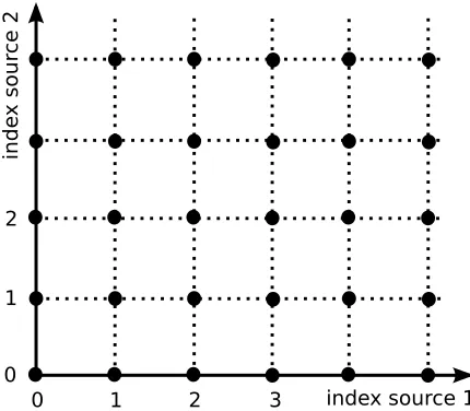
Figure 1: Schematic ordering of the optimal functions for SFA. For an unrestricted function space and statistically independent sources, the optimal functions for SFA are products of harmonics, each of which depends on one of the sources only. In the case of two sources, the optimal functions can therefore be arranged schematically on a 2-dimensional grid, where every grid point represents one function and its coordinates in the grid are the indices of the harmonics that are multiplied to form the function. Because the 0-th harmonic is the constant, the functions on the axes are simply the harmonics themselves and therefore depend on one of the sources only. Moreover, the grid points (1,0) and (0,1) are monotonic functions of the sources and therefore a good representative thereof. It is these solutions that the xSFA algorithm is designed to extract. Note that the scheme also contains an ordering by slowness: All functions to the upper right of a given function have higher ∆-values and therefore vary more quickly.

Theorem 1 Let gαi (i∈N) be the normalized eigenfunctions of the operatorsDα, that is,

the set of functions gαi that fulfill the eigenvalue equations

Dαgαi =λαigαi (10)

with the boundary conditions

pαKα∂αgαi = 0 (11)

and the normalization condition

(gαi, gαi)α:=hgαi2 isα = 1.

Then, the product functions

gi(s) :=

Y

α

gαiα(sα)

form a set of (normalized) eigenfunctions to the full operator D with the eigenvalues

λi=

X

α

and thus those gi with the smallest eigenvalues λi are the optimal functions for SFA. Here,

i = (i1, ..., iS) ∈ NS denotes a multi-index that enumerates the eigenfunctions of the full

eigenvalue problem.

In the following, we assume that the eigenfunctions gαi are ordered by their eigenvalue

and refer to them as the harmonicsof the sourcesα. This is motivated by the observation

that in the case wherepα andKα are independent ofsα, that is, for a uniform distribution,

the eigenfunctions gαi are harmonic oscillations whose frequency increases linearly with i

(see below). Moreover, we assume that the sourcessα are ordered according to slowness, in

this case measured by the eigenvalueλα1 of their lowest non-constant harmonicgα1. These

eigenvalues are the ∆-values of the slowest possible nonlinear point transformations of the sources.

The key result of theorem 1 is that in the case of statistically independent sources, the output signals are products of harmonics of the sources. Note that the constant func-tion gα0(sα) = 1 is an eigenfunction with eigenvalue 0 to all the eigenvalue problems (10).

As a consequence, the harmonicsgαi of the single sources are also eigenfunctions to the full

operator D (with the index i = (0, ...,0, iα = i,0, ...,0)) and can thus be found by SFA.

Importantly, the lowest non-constant harmonic of the slowest source (i.e., g(1,0,0,...) =g11)

is the function with the smallest overall ∆-value (apart from the constant) and thus the first function found by SFA. In the next sections, we show that the lowest non-constant harmonics gα1 reconstruct the sources up to a monotonic and thus invertible point

trans-formation and that in the case of sources with Gaussian statistics they even reproduce the sources exactly.

3.3 The First Harmonic Is A Monotonic Function Of The Source

The eigenvalue problem (10,11) has the form of a Sturm-Liouville problem (Courant and Hilbert, 1989) and can easily be rewritten to have the standard form for these problems:

∂αpαKα∂αgαi+λαipαgαi

(10,9)

= 0, (12)

with pαKα∂αgαi

(11)

= 0 for sα ∈ {a, b}. (13)

Here, we assume that the sourcesαis bounded and takes on values on the intervalsα∈[a, b].

Note that bothpαandpαKαare positive for allsα. Sturm-Liouville theory states that (i) all

eigenvalues are positive (Courant and Hilbert, 1989), (ii) the solutions gαi, i ∈ N0 of this

problem are oscillatory and (iii) gαi has exactly i zeros on ]a, b[ if the gαi are ordered by

increasing eigenvalue λαi (Courant and Hilbert, 1989, Chapter VI, §6). In particular, gα1

has only one zero ξ ∈]a, b[. Without loss of generality we assume that gα1 <0 for sα < ξ

and gα1>0 forsα > ξ. Then Equation (12) implies that

∂αpαKα∂αgα1=−λαpαgα1 <0 forsα > ξ

=⇒ pαKα∂αgα1 is monotonically decreasing on ]ξ, b] (13)

=⇒ pαKα∂αgα1 >0 on ]ξ, b[

=⇒ ∂αgα1 >0 on ]ξ, b[, because pαKα>0

A similar consideration for s < ξ shows that gα1 is also monotonically increasing on ]a, ξ[.

Thus,gα1 is monotonic and invertible on the whole interval [a, b]. Note that the monotony

of gα1 is important in the context of blind source separation, because it ensures that not

only some of the output signals of SFA depend on only one of the sources (the harmonics), but that there should actually be some (the lowest non-constant harmonics) that are very similar to the source itself.

3.4 Gaussian Sources

We now consider the situation that the sources are reversible Gaussian stochastic processes, (i.e., that the joint probability density ofs(t) ands(t+ dt) is Gaussian and symmetric with respect tos(t) ands(t+ dt)). In this case, the instantaneous values of the sources and their temporal derivatives are statistically independent, that is, ps˙α|sα( ˙sα|sα) = ps˙α( ˙sα). Thus, Kα is independent of sα, that is, Kα(sα) = Kα = const. Without loss of generality we

assume that the sources have unit variance. Then the probability density of the source is given by

pα(sα) =

1

√

2πe

−s2α/2

and the eigenvalue Equations (12) for the harmonics can be written as

∂αe−s

2 α/2_∂

αgαi+

λαi

Kα

e−s2α/2_g

αi = 0.

This is a standard form of Hermite’s differential equation (see Courant and Hilbert, 1989, Chapter V,§ 10). Accordingly, the harmonics gαi are given by the (appropriately

normal-ized) Hermite polynomialsHi of the sources:

gαi(sα) =

1

√

2i_i!Hi

sα

√

2

.

The Hermite polynomials can be expressed in terms of derivatives of the Gaussian distri-bution:

Hn(x) = (−1)nex

2

∂_xne−x2.

It is clear that Hermite polynomials fulfill the boundary condition

lim

sα→∞

Kαpα∂αgαi = 0,

because the derivative of a polynomial is again a polynomial and the Gaussian distribution decays faster than polynomially as |sα| → ∞. The eigenvalues depend linearly on the

indexi:

λαi =iKα. (14)

The most important consequence is that the lowest non-constant harmonics simply repro-duce the sources: gα1(sα) = 1/

√

2H1(sα/

√

2) =sα. Thus, for Gaussian sources, some of the

3.5 Uniformly Distributed Sources

Another canonical example for which the eigenvalue Equation (10) can be solved analyt-ically is the case of uniformly distributed sources, that is, the case where the probability distribution ps,s˙ is independent of son a finite interval and zero elsewhere. Consequently,

neitherpα(sα) nor Kα(sα) can depend onsα, that is, they are constants. Note that such a

distribution may be difficult to implement by a real differentiable process, because the veloc-ity distribution should be different at boundaries that cannot be crossed. Nevertheless, this case provides an approximation to cases, where the distribution is close to homogeneous.

Letsαtake values in the interval [0, Lα]. The eigenvalue Equation (12) for the harmonics

is then given by

Kα∂α2gαi+λαigαi = 0

and readily solved by harmonic oscillations:

gαi(sα) =

√

2 cos

iπsα

Lα

.

The ∆-value of these functions is given by

∆(gαi) =λαi =Kα

π

Lα

i

2

.

Note the similarity of these solutions with the optimal free responses derived by Wiskott (2003b).

3.6 Summary: Results Of The Theory

The following key results of the theory form the basis of the xSFA algorithm:

• For an unrestricted function space, the output signals generated by the optimal func-tions of SFA are independent of the nonlinear mixture, given the same original sources.

• The optimal functions of SFA are products of functionsgαi(sα), each of which depends

on only one of the sources. We refer to the function gαi as the i-th harmonic of the

sourcesα.

• The slowest non-constant harmonic is a monotonic function of the associated source. It can therefore be considered a good representative of the source.

• If the sources have stationary Gaussian statistics, the harmonics are Hermite poly-nomials of the sources. In particular, the lowest harmonic is then simply the source itself.

4. An Algorithm For Nonlinear Blind Source Separation

According to the theory, some of the output signals of SFA should be very similar to the sources. Therefore, the problem of nonlinear BSS can be reduced to selecting those output signals of SFA that correspond to the first non-constant harmonics of the sources. In this section, we propose and test an algorithm that should ideally solve this problem. In the following, we sometimes refer to the first non-constant harmonics simply as the “sources”, because they should ideally be very similar.

4.1 The xSFA Algorithm

The extraction of the slowest source is rather simple: According to the theory, it is well represented by the first (i.e., slowest) output signal of SFA. Unfortunately, extracting the second source is more complicated, because higher order harmonics of the first source may vary more slowly that the second source.

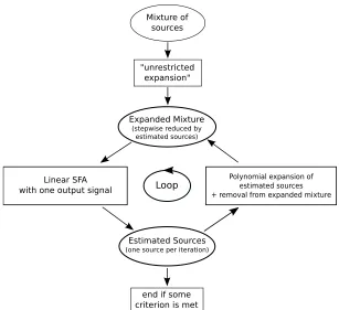
The idea behind the algorithm we propose here is that once we know the first source, we also know all its possible nonlinear transformations, that is, its harmonics. We can thus remove all aspects of the first source from the SFA output signals by projecting the latter to the space that is uncorrelated to all nonlinear versions of the first source. In the grid arrangement shown in Figure 1, this corresponds to removing all solutions that lie on one of the axes. The remaining signals must have a dependence on the second or even faster sources. The slowest possible signal in this space is then generated by the first harmonic of the second source, which we can therefore extract by means of linear SFA. Once we know the first two sources, we can proceed by calculating all the harmonics of the second source and all products of the harmonics of the first and the second source and remove those signals from the data. The slowest signal that remains then is the first harmonic of the third source. Iterating this scheme should in principle yield all the sources.

The structure of the algorithm is the following (see also Figure 2):

1. Start with the first source: i= 1.

2. Apply a polynomial expansion of degreeNSFA to the mixture to obtain the expanded mixturez.

3. Apply linear SFA to the expanded mixture z and store the slowest output signal as an estimate ˜si of source i.

4. Stop if the desired number of sources has been extracted (i=S).

5. Apply a polynomial expansion of degreeNnlto the estimated sources ˜s1,...,iand whiten

the resulting signals. We refer to the resulting nonlinear versions of the first sources asnk, k∈ {1, ..., Nexp}, whereNexpdenotes the dimension of a polynomial expansion

of degree Nnl of isignals.

6. Remove the nonlinear versions of the firstisources from the expanded mixturez

zj(t)←zj(t)−

Nexp

X

k=1

Figure 2: Illustration of the xSFA algorithm. The mixture of the input signals is first subjected to a nonlinear expansion that should be chosen sufficiently powerful to allow (a good approximation of) the inversion of the mixture. An estimate of the first source is then obtained by applying linear SFA to the expanded data. The remaining sources are estimated iteratively by removing nonlinear versions of the previously estimated sources from the expanded data and reapplying SFA. If the number of sources is known, the algorithm terminates when estimates of all sources have been extracted. If the number of sources is unknown, other termination criteria might be more suitable (not investigated here).

and remove principal components with a variance below a given threshold .

7. To extract the next source, increaseiby one and go to step 2, using the new expanded signals z.

Note that the algorithm is a mere extension of SFA in that it does not include new objectives or constraints. We therefore term it xSFA for eXtended SFA.

4.2 Simulations

4.2.1 Sources

Audio signals: We first evaluated the performance of the algorithm on two different test sets of audio signals. Data set A consists of excerpts from 14 string quartets by B´ela Bart´ok. Note that these sources are from the same CD and the same composer and contain the same instruments. They can thus be expected to have similar statistics. Differences in the ∆-values should mainly be due to short-term nonstationarities. This data set provides evidence that the algorithm is able to distinguish between signals with similar global statistics based on short-term fluctuations in their statistics.

Data set B consists of 20 excerpts from popular music pieces from various genres, ranging from classical music over rock to electronic music. The statistics of this set is more variable in their ∆-values, in particular they remain different even for long sampling times.

All sources were sampled at 44,100 Hz and 16 bit, that is, with CD-quality. The length of the samples was varied to assess how the amount of training data affects the performance of the algorithm.

Artificial data: To test how the algorithm would perform in tasks where more than two sources need to be extracted, we generated 6 artificial source signals with different temporal statistics. The sources were colored noise, generated by (i) applying a fast Fourier transform to white noise signals of lengthT, (ii) multiplying the resulting signals with exp(−f2/2σ_i2) (wheref denotes the frequency) and (iii) inverting the Fourier transform. The parameterσi

controls the ∆-values of the sources (∆≈σ_i2) and was chosen such that the ∆-values were roughly equidistant: σi =

√

i₅₀T + 1.

4.2.2 Nonlinear Mixtures

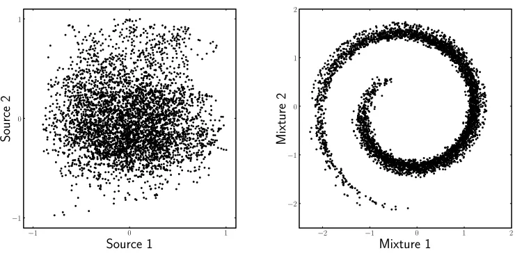
Audio signals: We subjected all possible pairs of sources within a data set to a nonlinear invertible mixture that was previously used by Harmeling et al. (2003) and Blaschke et al. (2007):

x1(t) = (s2(t) + 3s1(t) + 6) cos(1.5πs1(t)),

x2(t) = (s2(t) + 3s1(t) + 6) sin(1.5πs1(t)). (15)

Figure 3 illustrates the spiral-shaped structure of this nonlinearity. This mixture is only invertible if the sources are bounded between -1 and 1, which is the case for the audio data we used. The mixture (15) is not symmetric in s1 and s2. Thus, for every pair of sources,

there are two possible mixtures and we have tested both for each source pair.

We have also tested the other nonlinearities that Harmeling et al. (2003) have applied to two sources, as well as post-nonlinear mixtures, that is, linear mixture followed by a point nonlinearity. The performance was similar for all mixtures tested without any tuning of parameters (data not shown). Moreover, the performance remained practically unchanged when we used linear mixtures or no mixture at all. This is in line with the argument that the mixture should be irrelevant to SFA if the function space F is sufficiently rich (see section 3).

Separation of more than two sources: For the simulations with more than two sources, we created a nonlinear mixture by applying a nonlinear mixture twice. The basic post-nonlinear mixture is generated by first applying a random rotation Oij to the sources si

Figure 3: The spiral-shaped structure of the nonlinear mixture. Panel A shows a scatter plot of two sources from data set A. Panel B shows a scatter plot of the nonlinear mixture we used to test the algorithm.

arctangent as a nonlinearity:

Mi(s) = arctan



ζ−1 

 X

j

Oijsj



 

 ,

with a parameterζthat controls the strength of the nonlinearity. We normalized the sources to have zero mean and unit variance to ensure that the degree of nonlinearity is roughly the same for all combinations of sources and chose ζ = 2.

This nonlinearity was applied twice, with independently generated rotations, and a normalization step to zero mean and unit variance before each application.

4.2.3 Simulation Parameters

There are three parameters in the algorithm: the degreeNSFA of the expansion used for the first SFA step, the degree Nnl of the expansion for the source removal and the threshold for the removal of directions with negligible variance.

For the simulations with more than two sources, we used a polynomial expansion of degree NSFA = 3.

Degree of the expansion for source removal: For the simulations with two sources, we expanded the estimate for the first source in polynomials of degree Nnl = 20, that is, we projected out 20 nonlinear versions of the first source. Using fewer nonlinear versions does not alter the results significantly, as long as the expansion is sufficiently complex to remove those harmonics of the first source that have smaller ∆-values than the second source. Using higher expansion degrees sometimes leads to numerical instabilities, which we accredit to the extremely sparse distribution that results from the application of very high monomials. For the separation of more than two sources, all polynomials of degree Nnl = 4 of the already estimated sources were projected out.

Variance threshold: After the removal of the nonlinear versions of the first source, there is at least one direction with vanishing variance. To avoid numerical problems caused by singularities in the covariance matrices, directions with variance below = 10−7 were removed. For almost all source pairs, the only dimension that had a variance below after the removal was the trivial direction of the first estimated source.

The simulations were done in Python using the modular toolkit for data processing (MDP) developed by Zito et al. (2008). The xSFA algorithm is included in the current version of MDP (http://mdp-toolkit.sourceforge.net).

4.2.4 Performance Measure

For stationary Gaussian sources, the theory predicts that the algorithm should reconstruct the sources exactly. In most applications, however, the sources are neither Gaussian nor stationary (at least not on the time scales we used for training). In this case the algorithm cannot be expected to find the sources themselves, but rather a nonlinearly transformed version of the sources, ideally their lowest harmonics. Thus, the correlation between the output signals of the algorithm and the sources is not necessarily the appropriate measure for the quality of the source separation. Therefore, we also calculated the lowest harmonicsgα1

of the sources by applying SFA with a polynomial expansion of degree 11 to the individual sources separately and then calculated the correlations between the output signals of the algorithm and both the output signals of the harmonicsyα1(t) =gα1(sα(t)) and the sources

themselves. In addition to the correlation coefficient, we also calculated the signal-to-noise ratio.

4.2.5 Simulation Results

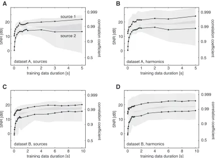
0 1 2 3 4 5 training data duration [s]

SN R [ d B] 0 10 20 A B C D co rre la tio n co e ffi ci e n t 0.999 0.99 0.9 0.5 co rre la tio n co e ffi ci e n t 0.999 0.99 0.9 0.5 co rre la tio n co e ffi ci e n t 0.999 0.99 0.9 0.5 co rre la tio n co e ffi ci e n t 0.999 0.99 0.9 0.5 SN R [ d B] 0 10 20 SN R [ d B] 0 10 20 SN R [ d B] 0 10 20

0 1 2 3 4 5

training data duration [s]

0 2 4 6 8 10

training data duration [s]

0 2 4 6 8 10

training data duration [s]

dataset A, sources dataset A, harmonics

dataset B, sources dataset B, harmonics

source 1

source 2

Figure 4: Performance of the algorithm as a function of the duration of the training data. The curves show the median of the distribution of correlation coefficients between the reconstructed and the original sources, as well as the corresponding signal-to-noise ratio (SNR). Grey-shaded areas indicate the region between the 25th and the 75th percentile of the distribution of the correlation/SNR. Statistics cover all possible source pairs that can be simulated (data set A: 14 sources→ 182 source pairs, data set B: 20 sources → 380 source pairs). Panels A and B show results for data set A, panels C and D for data set B. Panels A and C show the ability of the algorithm to reconstruct the sources themselves, while B and D show the performance when trying to reconstruct the slowest harmonics of the sources. Note the difference in time scales.

co

rre

la

tio

n

co

e

ffi

ci

e

n

t

SN

R

[

d

B]

training data duration [10 samples]4

2 4 6 8 10

0

0.99

0.9

0.5

0.1 0

10

-10

-20

source 1

source 6

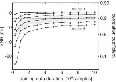
Figure 5: Performance of the algorithm for multiple sources. The curves show the median of the distribution of correlation coefficients between the reconstructed and the orginal six sources, as well as the corresponding signal-to-noise ratio (SNR). The grey-shaded area indicates the region between the 25th and the 75th percentile of the distribution of the correlation/SNR for the 4th source. The percentiles for the other sources are similar but not shown for reasons of graphical clarity. Statistics cover 50 repetitions with independently generated sources. The dashed grey line indicates the performance of a linear regression.

For data set B, longer training times of at least 2s were necessary to reach a similar performance as for data set A. Further research is necessary to assess the reasons for this. Again, the estimated sources are more similar to the slowest harmonics of the sources than to the sources themselves. The reconstruction performance increases with the duration of the training data. For this data set, the prominent divergence of the percentiles for data set A is not observed.

The performance of xSFA is significantly better than that of independent slow feature analysis (ISFA; Blaschke et al., 2007), which also relies on temporal correlations and was reported to reconstruct both sources with CC>0.9 for about 70% of the source pairs. For our data sets, both sources were reconstructed with a correlation of more than 0.9 for more than 90% of the source pairs, if the duration of the training data was sufficiently large. Moreover, it is likely that the performance of xSFA can be further improved, for example, by using more training data or different function spaces.

The algorithm is relatively fast: On a notebook with 1.7GHz, the simulation of the 182 source pairs for data set A with 0.2s training sequences takes about 380 seconds, which corresponds to about 2.1s for the unmixing of a single pair.

with increasing amount of training data. For 105 training data points, four of six estimated sources have a correlation coefficient with the original source that is larger than 0.9. The performance of a supervised linear regression between the sources and the mixture happens to be close to 0.9. For the first four extracted sources, xSFA is thus performing better than any linear technique could.

5. Practical Limitations

There are several reasons why the algorithm can fail, because some of the assumptions underlying the theory are not necessarily fulfilled in simulations. In the following, we discuss some of the reasons for failures. The main insights are summarized at the end of the section.

5.1 Limited Sampling Time

The theory predicts that some of the output signals reproduce the harmonics of the sources exactly. However, problems can arise if eigenfunctions have (approximately) the same eigen-value. For example, assume that the sources have the same temporal statistics, so that the ∆-value of their slowest harmonics gµ1 is equal. Then, there is no reason for SFA to prefer

one signal over the other.

Of course, in practice, two signals are very unlikely to have exactly the same ∆-value. However, the difference may be so small that it cannot be resolved because of limited sampling. To get a feeling for how well two sources can be distinguished, assume there were only two sources that are drawn independently from probability distributions with ∆-values ∆ and ∆ +δ. Then linear SFA should ideally reproduce the sources exactly. However, if there is only a finite amount of data, say of total duration T, the ∆-values of the signals can only be estimated with finite precision. Qualitatively, we can distinguish the sources when the standard deviation of the estimated ∆-value is smaller than the difference δ in the “exact” ∆-values. It is clear that this standard deviation depends on the number of data points roughly as 1/√T. Thus the smallest difference δmin in the ∆-values that can

be resolved has the functional dependence

δmin ∼∆α

1

√

T .

The reason why the smallest distinguishable difference δ must depend on the ∆-value is that subsequent data points are not statistically independent, because the signals have a temporal structure. For slow signals, that is, signals with a small ∆-values, the estimate of the ∆-value is less precise than for quickly varying signals, because the finite correlation time of the signals impairs the quality of the sampling. For dimensionality reasons, the exponentα has to take the value α= 3/4, yielding the criterion

δmin

∆ ∼

1

p

T√∆

.

spectrum centered at zero):

∆(y) = 1 T

Z

˙

y2dt= 1

T

Z

ω2|y(ω)|2_{dω , (16)}

wherey(ω) denotes the Fourier transform of y(t). However, the inverse width of the power spectrum is an operative measure for the correlation timeτ of the signal, leaving us with a correlation timeτ ∼1/√∆. With this in mind, the criterion (16) takes a form that is much easier to interpret:

δmin

∆ ∼

r

τ

T =

1

√

Nτ

. (17)

The correlation timeτ characterizes the time scale on which the signal varies, so intuitively, we can cut the signal into Nτ = T /τ “chunks” of duration τ, which are approximately

independent. Equation (17) then states that the smallest relative difference in the ∆-value that can be resolved is inversely proportional to the square root of the number Nτ of

independent data “chunks”.

If the difference in the ∆-value of the predicted solutions is smaller than δmin, SFA is

likely not to find the predicted solutions but rather an arbitrary mixture thereof, because the removal of random correlations and not slowness is the essential determinant for the solution of the optimization problem. Equation (17) may serve as an estimate of how much training time is needed to distinguish two signals. Note however, that the validity of (17) is questionable for nonstationary sources, because the statistical arguments used above are not valid.

Using these considerations, we can estimate the order of magnitude of training data that is needed for the data sets we used to evaluate the performance of the algorithm. For both data sets, the ∆-values of the sources were on the order of 0.01, which corresponds to an autocorrelation time of approximately 1/√0.01 = 10 samples. Those sources of data set A that were most similar differed in ∆-value by δ/∆ ∼ 0.05, which requires Nτ = (1/0.05)2 = 400. This corresponds to∼4000 samples that are required to distinguish

the sources, which is similar to what was observed in simulations. In data set B, the problem is not that the sources are too similar, but rather that they are too different in ∆-value, which makes it difficult to distinguish between the products of the second source and harmonics of the first and the second source alone. The ∆-values often differ by a factor of 20 or more, so that the relative difference between the relevant ∆-values is again on the order of 5%. In theory, the same amount of training data should therefore suffice. However, if the sources strongly differ in ∆-value, many harmonics need to be projected out before the second source is accessible, which presumably requires a higher precision in the estimate of the first source. This might be one reason why significantly more training data is needed for data set B.

5.2 Sampling Rate

low sampling rates this renders techniques like SFA that are based on short-term temporal correlations useless.

For discrete data, the temporal derivative is usually replaced by a difference quotient:

˙

y(t)≈ y(t+ ∆t)−y(t)

∆t ,

where y(t+ ∆t) and y(t) are neighboring sample points and ∆t is given by the inverse of the sampling rate r. The ∆-value can then be expressed in terms of the variance of the signal and its autocorrelation function:

∆(y) =hy˙2it≈

2 ∆t2 hy

2_i

t− hy(t+ ∆t)y(t)it

= 2r2 hy2it− hy(t+ ∆t)y(t)it

. (18)

If the sampling is too low, the signal effectively becomes white noise. In this case, the term that arises from the time-delayed correlation vanishes, while the variance remains constant. Thus, for small sampling rates, the ∆-value depends quadratically on the sampling rate, while it saturates to its “real” value if the sampling rate is increased. This behavior is illustrated in Figure 6A. Note that two signals with different ∆-values for sufficient sampling rate may have very similar ∆-value when the sampling is decreased too drastically. Intuitively, this is the case if the sampling rate is so low that both signals are (almost) white noise. In this case, there are no temporal correlations that could be exploited, so that SFA returns a random mixture of the signals.

The number of samples N that can be used for training is limited by the working memory of the computer and/or the available CPU time. Thus, for a fixed maximal number of training samples N, the sampling rate implicitly determines the maximal training time

T =N/r. The training time, in turn, determines the minimal relative difference in ∆-value

that can be distinguished (cf. Equation (17)). Thus, for a fixed number of sample points, the minimal relative difference in ∆-value that can be resolved is proportional to 1/√T ∼√r. But why do low sampling rates lead to a better resolution? The reason is that for high sampling rates, neighboring data points have essentially the same value. Thus, they do not help in estimating the ∆-value, because they do not carry new information.

In summary, the sampling rate should ideally be in an intermediate regime. If the sampling rate is too low, the signals become white noise and cannot be distinguished, while too high sampling rates lead to high computational costs without delivering additional information. This is illustrated in Figure 6B.

5.3 Density Of Eigenvalues

A B

Figure 6: Influence of the sampling rate. (A) Qualitative dependence of the ∆-value of two different signals on the sampling rate. For very low sampling rates, both signals become white noise and the ∆-value quadratically approaches zero. Signals that have different ∆-values for sufficiently high sampling rates may therefore not be distinguished if the sampling rate is too low. The dotted lines indicate the “real” ∆-values of the signals. Note: It may sound counterintuitive that the ∆-value drops to zero with decreasing sampling rate, as white noise should be regarded as a quickly varying signal. This arises from taking the sampling rate into account in the temporal derivative (18). If the derivative is simply replaced by the difference between adjacent data points, the ∆-value approaches 2 as the sampling rate goes to zero and decreases with the inverse square of the sampling rate as the sampling rate becomes large. (B) Sampling rate dependence of the “resolution” of the algorithm for a fixed number of training samples. The solid line shows the qualitative dependence of the relative difference in ∆-value of two signals as a function of the sampling rate and the dashed line shows the qualitative behavior of the minimal relative difference in ∆-value that can be resolved. The signals can only be separated by SFA if the resolvable difference (dashed) is below the expected relative difference (solid). Therefore an intermediate sampling is more efficient. The dotted line indicates the “real” ratio of the ∆-values.

In the Gaussian approximation, the ∆-values of the harmonics are equidistantly spaced, cf. Equation (14). As the ∆-value ∆i of the full product solution gi is the sum of the

∆-values of the harmonics, the condition ∆i<∆ restricts the indexito lie below a hyperplane

with the normal vectorn= (λ11, ..., λS1)∈RS: X

µ

iµλµ1 =i·n<∆. (19)

Because the indices are homogeneously distributed in index space with density one, the expected number of solutions with ∆<∆0 is simply the volume of the subregion in index

space for which Equation (19) is fulfilled:

R(∆) = 1

S!

S

Y

µ=1

∆

λµ1

The density of the eigenvalues is then given by

ρ(∆) = ∂R(∆)

∂∆ =

1 (S−1)!

" Y

µ

1

λµ1

#

∆S−1.

As the density of the eigenvalues can be interpreted as the inverse of the expected distance between the ∆-values, the distance and thus the separability of the solutions with a given amount of data declines as 1/∆S−1. In simulations, we can expect to find the theoretically predicted solutions only for the slowest functions, higher order solutions tend to be linear mixtures of the theoretically predicted functions. This is particularly relevant if there are many sources, that is, ifS is large.

If the sources are not Gaussian, the dependence of the density on the ∆-value may have a different dependence on ∆ (e.g., for uniformly distributed sources ρ(∆) ∼∆S/2−1). The problem of decreasing separability, however, remains.

5.4 Function Space

An assumption of the theory is that the function space accessible to SFA is unlimited. However, any application has to restrict the function space to a finite dimensionality. If the function space is ill-chosen in that it cannot invert the mixture that generated the input data from the sources, it is clear that the theory can no longer be valid.

Because the nature of the nonlinear mixture is not knowna priori, it is difficult to choose an appropriate function space. We used polynomials with relatively high degree. A problem with this choice is that high polynomials generate extremely sparse data distributions. Depending on the input data at hand, it may be more robust to use other basis functions such as radial basis functions or kernel approaches (B¨ohmer et al., 2012), although for SFA, these tend to be computationally more expensive.

The suitability of the function space is one of the key determinants for the quality of the estimation of the first source. If this estimate is not accurate but has significant contributions from other sources, the nonlinear versions of the estimate that are projected out are not accurate, either. The projection step may thus remove aspects of the second source and thereby impair the estimate of the second source. For many sources, these errors accumulate so that estimates for faster sources will not be trustworthy, an effect that is clearly visible in the simulations with more sources. This problem might be further engraved by the increasing eigenvalue density discussed above.

5.5 Summary

In summary, we have discussed four factors that have an influence on simulation results:

• Limited sampling time: Whether the algorithm can distinguish two sources with similar ∆-values depends on the amount of data that is available. More precisely, to separate two sources with ∆-values ∆ and ∆ +δ, the durationT of the training data should be on the order of T ∼τ(∆/δ)2 or more. Here, τ is the autocorrelation time of the signals, which can be estimated from the ∆-value of the sources: τ ≈1/√∆.

subsequent data points. If the numberT of samples that can be used is limited by the memory capacity of the computer, very high sampling rates can be a disadvantage, be-cause the correlation timeτ (measured in samples) of the data is long. Consequently, the number T /τ of “independent data chunks” is smaller than with lower sampling rates, which may impair the ability of the algorithm to separate sources with similar ∆-values (see previous point).

• Density of eigenvalues: The problem of similar ∆-values is not only relevant when the sources are similar, because the algorithm also needs to distinguish the faster sources from products of these sources with higher-order harmonics of the lower sources. To estimate how difficult this is, we have argued that, for the case of Gaussian sources, the expected difference between the ∆-values of the output of SFA declines as 1/∆S−1, where S is the number of sources. Separating a source from the prod-uct solutions of lower-order sources therefore becomes more difficult with increasing number of sources.

• Function space: Another important influence on the performance of the system is the choice of the function spaceF for SFA. Of course,F has to be chosen sufficiently rich to allow the inversion of the nonlinear mixture. According to the theory additional complexity of the function spaces should not alter the results and we have indeed found that the system is rather robust to the particular choice of F, as long as it is sufficiently complex to invert the mixture. We expect, however, that an extreme increase in complexity leads to (a) numerical instabilities (in particular for polynomial expansions as used here) and (b) overfitting effects.

6. Relation To Other Nonlinear BSS Algorithms

Because xSFA is based on temporal correlations, in a very similar way as the kernel-TDSEP (kTSDEP) algorithm presented by Harmeling et al. (2003), one could expect the two algorithms to have similar performance. By using the implementation of the kTDSEP algorithm made available by the authors,2 we compared kTDSEP with xSFA on the audio signals from data set A in the case of the spiral mixture (15). For the best parameter setting we could identify, kTDSEP was able to recover both sources (with correlation>0.9) for only 20% of the signal pairs, while xSFA recovered both sources for more than 90% of the source pairs with the same training data. This result was obtained using a training data duration of 0.9 s, 25 time-shifted covariance matrices, a polynomial kernel of degree 7, and k-means clustering with a maximum of 10000 points considered. Results depended strongly but not systematically on training data duration. A regression analysis for a few of the failure cases revealed that the sources were present among the extracted components, but not properly selected, suggesting that the poor performance was primarily caused by a failure of the automatic source selection approach of Harmeling et al. (2003). The kTDSEP algorithm would resemble xSFA even more if kernel PCA were used instead of k-means clustering for finding a basis in the kernel feature space. Using kernel PCA, however, yields worse results: both sources were recovered at best in 5% of the signal pairs. The influence of the kernel

choice (kernel PCA/k-means) on the performance could be due to numerical instabilities and small eigenvalues, which we avoid in xSFA by using singular value decomposition with thresholding in the SFA dimensionality reduction step.

Almeida (2003) has suggested a different approach (MISEP) that uses a multilayer per-ceptron to extend the maximum entropy ansatz of Bell and Sejnowski (1995) to the nonlinear case. MISEP has been shown to work in an application to real data (Almeida, 2005). In our hands, MISEP was not able to solve the spiral-shaped nonlinear mixture described in Section 4, however, exactly because of the problems described by Hyv¨arinen and Pajunen (1999): it converges to a nonlinear mixture of the sources that generates statistically in-dependent output signals. Conversely, xSFA fails to solve the image unmixing problem on which MISEP was successful (Almeida, 2005), probably because of low-frequency com-ponents that introduce correlations between the images (Ha Quang and Wiskott, 2013). Whether an information-theoretic ansatz like MISEP or a temporal approach like xSFA is more suitable therefore seems to depend on the problem at hand.

Zhang and Chan (2008) have suggested that the indeterminacies of the nonlinear BSS problem could be solved by a minimal nonlinear distortion (MND) principle, which assumes that the mixing function is smooth. To exploit this, they added a regularization term to common nonlinear ICA objective functions (including that of MISEP). They investigated both a global approach that punishes deviations of the unmixing nonlinearity from the best linear solution and a local approach that favors locally smooth mappings. The latter is remotely related to xSFA, which also tries to enforce smooth mappings, but measures smoothness in time rather than directly in the unmixing function. The MND ansatz applies to arbitrary functions, while xSFA is limited to time-varying data. On the other hand, the temporal smoothness constraint of xSFA could extend to problems where the original sources are smooth, but the mixing function is not.

A nonlinear BSS approach that is even more akin to SFA is the diffusion-map ansatz of Singer and Coifman (2008). Diffusion maps and Laplacian eigenmaps are closely related to SFA (Sprekeler, 2011). A key difference lies in the choice of the local metrics of the data, which is dictated by the temporal structure for SFA (the matrix Kαβ can be thought of

as an inverse metric tensor), but hand-chosen for diffusion maps. Singer & Coifman made a data-driven choice for the metric tensor through local inspection of the data manifold, and showed that the resulting diffusion maps can reconstruct the original sources in a toy example (Singer and Coifman, 2008) and extract slowly varying manifolds in time series data (Singer et al., 2009).3

7. Discussion

In this article, we have extended previous theoretical results on SFA to the case where the input data are generated from a set of statistically independent sources. The theory shows that (a) the optimal output of SFA consists of products of signals, each of which depends on a single source only and that (b) some of these harmonics should be monotonic functions of the sources themselves. Based on these predictions, we have introduced the xSFA algorithm to iteratively reconstruct the sources, in theory from arbitrary invertible mixtures. Simulations have shown that the performance of xSFA is substantially higher

than the performance of independent slow feature analysis (ISFA; Blaschke et al., 2007) and kTDSEP (Harmeling et al., 2003), other algorithms for nonlinear BSS that also rely on temporal correlations.

xSFA is relatively robust to changes of parameters. Neither the degree of the expansion before the first SFA step nor the number of removed nonlinear versions of the first source need to be finely tuned, though both need to be within a certain range, so that the BSS problem can be solved without running into the overfitting or error accumulation problems discussed above. It should be noted, moreover, that polynomial expansions - as used here - become problematic if the degree of the expansion is too high. The resulting expanded data contain directions with very sparse distributions, which can lead (a) to singularities in the covariance matrix (e.g., for Gaussian signals with limited sampling,x20 _{and x}22 _are

almost perfectly correlated) and (b) to sampling problems for the estimation of the required covariances because the data are dominated by few data points with high values. Note, that this problem is not specific to the algorithm itself, but rather to the expansion type used. Other expansions such as radial basis functions may be more robust. The relative insensi-tivity of xSFA to parameters is a major advantage over ISFA, whose performance depended crucially on the right choice of a trade-off parameter between slowness and independence.

Many algorithms for nonlinear blind source separation are designed for specific types of mixtures, for example, for nonlinear mixtures (for an overview of methods for post-nonlinear mixtures see Jutten and Karhunen, 2003). In contrast, our algorithm should work for arbitrary instantaneous mixtures. As previously mentioned, we have performed simulations for a set of instantaneous nonlinear mixtures and the performance was similar for all mixtures. The only requirements are that the sources are distinguishable based on their ∆-value and that the function space accessible to SFA is sufficiently complex to invert the mixture. Note that the algorithm is restricted to instantaneous mixtures. It cannot invert convolutive mixtures because SFA processes its input instantaneously and is thus not suitable for a deconvolution task.

It would be interesting to see if the theory for SFA can be extended to other algorithms. For example, given the close relation of SFA to TDSEP (Ziehe and M¨uller, 1998), a variant of the theory may apply to the kernel version of TDSEP (Harmeling et al., 2003). In particular, it would be interesting to see whether the theory would suggest an alternative source selection algorithm for kTDSEP that is more robust.

In summary, we have presented a new algorithm for nonlinear blind source separation that is (a) independent of the mixture type, (b) robust to parameters, (c) underpinned by a rigorous mathematical framework, and (d) relatively reliable, as shown by the reconstruction performance for the examined cases.

Acknowledgments

Appendix A. Proof Of Theorem 1

The proof that all product functionsgi=Qαgαiα(sα) are eigenfunctions of the operatorD=

P

βDβ can be carried out directly:

Dgi(s) =   X β Dβ   Y α

gαiα(sα)

= X

β

D_βY

α

gαiα(sα)

= X

β

D_βgβiβ(sβ)

Y

α6=β

gαiα(sα)

(because Dβ is a differential operator w.r.t. sβ only)

= X

β

λβiβgβiβ(sβ)

Y

α6=β

gαiα(sα)

=



 X

β

λβiβ



 Y

α

gαiα(sα)

= λigi(s).

Because the product functions are eigenfunctions of the full operator D, the theory of Franzius et al. (2007, Theorems 1-5) applies, stating that the J product functions with the smallest eigenvalue, ordered by their eigenvalue, are the solutions of the optimization problem of SFA. The proof of this theory requires that the eigenfunctions form a complete set. Because the set of eigenfunctions for the individual operators Dα form a complete set

for the individual Sobolev space of functions depending on sα only, however (Courant and

Hilbert, 1989, §14), the product set gi is also a complete set for the product space.

Appendix B. Proof That Kαβ Is Diagonal

To prove that the matrixKαβ(s) is diagonal, we first need to prove that the mean temporal

derivative of any 1-dimensional signal given its value vanishes: hs˙i_s˙|s = R sp( ˙˙ s|s)d ˙s = 0. To do so, we assume that the distribution of the signal is stationary and that the signal is continuously differentiable. Because of the stationarity, the probability that the signal is smaller than a given values0 is constant:

0 = d

dt

Z s0

−∞ Z ∞

−∞

p(s,s)dsd ˙˙ s

=

Z s0

−∞ Z ∞

−∞

∂tp(s,s)dsd ˙˙ s

= −

Z s0

−∞ Z ∞

−∞

∂s[ ˙sp(s,s)] +˙ ∂s˙[¨sp(s,s))] dsd ˙˙ s

where we used the continuity equation∂tp(s,s) +˙ ∂s[ ˙sp(s,s)] +˙ ∂s˙[¨sp(s,s))] = 0. Using the˙

all s < s0, we get the desired result:

0 = −

Z ∞

−∞

˙

sp(s,s)d ˙˙ s

= −p(s)hs˙i_s˙|s.

Because the mean temporal derivative hs˙αis˙α|sα is zero for each signal, the matrix Kαβ =

hs˙αs˙βis˙|sis not only the matrix of the second moments of the velocity distribution given the

signal valuessbut its covariance matrix. Because the signals are statistically independent, they are necessarily uncorrelated, that is, their covariance matrix is diagonal.

References

L. Almeida. MISEP: Linear and nonlinear ICA based on mutual information. Journal of Machine Learning Research, 4:1297–1318, 2003.

L. Almeida. Separating a real-life nonlinear image mixture. Journal of Machine Learning Research, 6:1199–1229, 2005.

A. Bell and T. Sejnowski. An information maximization approach to blind separation and blind deconvolution. Neural Computation, 7:1129–1159, 1995.

P. Berkes and L. Wiskott. Slow feature analysis yields a rich repertoire of complex cells.

Journal of Vision, 5(6):579–602, 2005.

T. Blaschke, P. Berkes, and L. Wiskott. What is the relation between slow feature analysis and independent component analysis? Neural Computation, 18(10):2495–2508, 2006. T. Blaschke, T. Zito, and L. Wiskott. Independent slow feature analysis and nonlinear blind

source separation. Neural Computation, 19(4):994–1021, 2007.

W. B¨ohmer, S. Gr¨unew¨alder, H. Nickisch, and K. Obermayer. Generating feature spaces for linear algorithms with regularized sparse kernel slow feature analysis. Machine Learning, 89:67–86, 2012.

S. Choi. Differential learning algorithms for decorrelation and independent component analysis. Neural Networks, 19(10):1558–1567, Dec 2006.

R. Courant and D. Hilbert. Methods of Mathematical Physics, Part I. Wiley, 1989.

M. Franzius, H. Sprekeler, and L. Wiskott. Slowness and sparseness lead to place, head-direction, and spatial-view cells. PLoS Computational Biology, 3(8):e166, 2007.

M. Ha Quang and L. Wiskott. Multivariate slow feature analysis and decorrelation filtering for blind source separation. Image Processing, IEEE Transactions on, 22(7):2737–2750, 2013.

A. Hyv¨arinen and P. Pajunen. Nonlinear independent component analysis: Existence and uniqueness results. Neural Networks, 12(3):429–439, 1999.

A. Hyv¨arinen, J. Karhunen, and E. Oja. Independent Component Analysis. Wiley, 2001. C. Jutten and J. Karhunen. Advances in nonlinear blind source separation. Proc. of the 4th

Int. Symp. on Independent Component Analysis and Blind Signal Separation (ICA2003), pages 245–256, 2003.

A. Singer and R. Coifman. Non-linear independent component analysis with diffusion maps.

Applied and Computational Harmonic Analysis, 25(2):226–239, 2008.

A. Singer, R. Erban, I. G. Kevrekidis, and R. R. Coifman. Detecting intrinsic slow variables in stochastic dynamical systems by anisotropic diffusion maps.Proceedings of the National Academy of Sciences, 106(38):16090–16095, 2009.

H. Sprekeler. On the relation of slow feature analysis and Laplacian eigenmaps. Neural Computation, 23:3287–3302, 2011.

L. Wiskott. Learning invariance manifolds. In L. Niklasson, M. Bod´en, and T. Ziemke, editors, Proceedings of the 8th International Conference on Artificial Neural Networks, ICANN’98, Sk¨ovde, Perspectives in Neural Computing, pages 555–560, London, Sept. 1998. Springer. ISBN 3-540-76263-9.

L. Wiskott. Estimating driving forces of nonstationary time series with slow feature analysis. arXiv.org e-Print archive, http://arxiv.org/abs/cond-mat/0312317/, Dec. 2003a.

L. Wiskott. Slow feature analysis: A theoretical analysis of optimal free responses. Neural Computation, 15(9):2147–2177, 2003b.

L. Wiskott and T. Sejnowski. Slow feature analysis: unsupervised learning of invariances.

Neural Computation, 14:715–770, 2002.

K. Zhang and L. Chan. Minimal nonlinear distortion principle for nonlinear independent component analysis. Journal of Machine Learning Research, 9:2455–2487, 2008.

A. Ziehe and K.-R. M¨uller. TDSEP–an efficient algorithm for blind separation using time structure. Proc. Int. Conf. on Artificial Neural Networks (ICANN ’98), pages 675–680, 1998.