http://www.sciencepublishinggroup.com/j/jeee doi: 10.11648/j.jeee.20170503.14
ISSN: 2329-1613 (Print); ISSN: 2329-1605 (Online)
Optimal Location and Sizing of Distributed Generation for
Minimizing Power Loss Using Simulated Annealing
Algorithm
Salah Kamal EL-Sayed
Department of Electrical Power & Machines, Faculty of Engineering, Al-Azhar University, Cairo, Egypt
Email address:
To cite this article:
Salah Kamal EL-Sayed. Optimal Location and Sizing of Distributed Generation for Minimizing Power Loss Using Simulated Annealing Algorithm. Journal of Electrical and Electronic Engineering. Vol. 5, No. 3, 2017, pp. 104-110. doi: 10.11648/j.jeee.20170503.14
Received: May 15, 2017; Accepted: May 23, 2017; Published: June 21, 2017
Abstract:
Distributed Generation integration in electric power system is one of the options which give many benefits such that loss Reduction, peak saving, voltage profile improvement, stability and reliability improvement. The installation of DG units at non-optimal location can result in an increase in system losses, damaging voltage state. In this paper, simulated annealing Algorithm (SAA) techniqueis designed for optimally determining the location, sizing and numbers of distributed generations depending on power loss reduction and voltage profile improvement. The proposed technique is tested on IEEE 57- bus system to demonstrate the performance of the network after inserting the distributed generation in selected optimal location with optimal sizing. Results show the efficiency of the proposed algorithm in reducing power losses, improving voltage profile.Keywords: Distributed Generation, Power Loss, Voltage Profile, Simulated Annealing Algorithm (SAA)
1. Introduction
In the present days, electrical power demand is increasing rapidly, and generation can’t reach to the existing demand so it is need extra power or emergency power which must be connected in the distribution system. The performance of distribution system becomes inefficient due to the reduction in voltage magnitude and increase in distribution system losses. Distributed Generation integration in electric power system is one of the options which give many benefits such that loss Reduction, peak saving, voltage profile improvement, improvement of power system stability and reliability. Situation of DG units on the distribution network has been constantly studied to achieve several objectives with different types of DG in different test systems are studied in literature review. A load flow based on algorithm for reducing line loss and improving voltage profile is performed in [1]. Load flow algorithm is combined appropriately with GA technique as in [2]. Planning and operation of active distribution networks, with respect to placement and sizing of Distributed Generators are discussed with the help of a fuzzy logic methodology in [3] Renewable energy source DG
location based on voltage sensitivity index is illustrated in [4]. A simple and fast approach for allocation and size evaluation of distributed generation using ANN technique is done in [5]. optimal DG unit and capacitor placements in distribution systems are studied in [6] two innovative mathematic models are proposed to solve OPF problems and other methods like Bacterial Foraging Algorithm (BFA), bus-injection to branch-current (BIBC) and branch-current to bus voltage (BCBV) and Shuffled Frog Leaping Algorithm (SFLA) [7-8].
These algorithms have come into existence and almost succeeded in getting optimal or near optimal solution with operating constraints. But the problem associated with these techniques is increase in computational time with the improper selection of control parameters. Many approaches are proposed for allocation of Dispersed Generators and they are still in research and enlargement stage. Different types of the DG’s can be characterized as [9]:
Type I: DG capable of injecting real power only, like photovoltaic, fuel cells etc.
TypeIII: DG capable of injecting reactive power only to improve the voltage profile e.g. synchronous compensator.
Type IV: DG capable of injecting real but consuming reactive power, e.g. induction generators used in the wind farms.
The problem formulation of this paper introduces a simulated annealing Algorithm (SAA) technique for finding optimal location, sizing and numbers of Distributed Generation to obtain minimum losses of the power system network with voltage profile improvement. In this paper, Type I and II of DG will be used. This paper is organized as follows:
Section2, explain the Distributed Generation definitions, benefits, and technologies. In the section 3 the problem statement is described with the objective functions and inequality constraints. In the section 4, simulated annealing as artificial intelligence technique is illustrated to determine the optimal location, proper size and numbers of the DGs. After that, in section 5 the test system IEEE57-bus networks described and the impact of the DGs units on voltage profile and power losses is illustrated. In the last section, some relevant conclusions are given.
2. Distribution Generation
Distributed generators are small scale generators is usually connected to distribution system and located close to consumers. Normally Distributed Generators are in range of 1 kW ratings to 100 MW [10]. There are many definitions of the DG but have the same meaning, for example, the working group of CIGRE devoted to distributed generation defines distributed generation as all generation units with a maximum capacity of 50MW to 100MW [11], that are usually connected to the distribution network and which are neither centrally planned nor dispatched. The definition of the location of the distributed generation plants varies among different authors. Most authors define the location of DG at the distribution side of the network, some authors also include the customer's side, and some even include the transmission side of the network [10].
2.1. Benefits of Distributed Generation
Using of DGs has many advantages to the customers and the distribution systems and they also have negative effects sometimes.
The basic benefits of Distributed Generation are given as in [12]:
(1). Reduces the cost as there is no use of long transmission line.
(2). Reduces the complexity. (3). Environment friendly.
(4). Avoid the impact of massive grid failure.
(5). Easy to maintain and easy to operate as it consists of simple construction.
(6). Better power system quality and reliability. (7). The factor of high peak load shortage eliminates. (8). Improves the efficiency of providing electric power. The negative impacts of the performing of DG might be as
follows [12]:
(1). Unsteadiness of the voltage profile owing to the bi directional power flows.
(2). Unsteadiness of the voltage profile owing to the bidirectional quality of the supply.
(3). System frequency deviations; the installations of DG increase the burden on the system operator to maintain the system frequency.
(4). Less choice between costlier primary fuels; most DG technologies are based on gas.
2.2. Technologies for Distributed Generation
There are several technologies are used for distributed generation. Where large amounts of recently popped up generation technologies, The Distributed Generation technologies are as following in [12]:
(1). Wind Turbines. (2). Fuel Cells (3). Photovoltaic
(4). Reciprocating Engines. (5). Combustion Gas Turbines. (6). Micro turbines.
(7). Another renewable Includes thermal solar, small hydro, geothermal, ocean
3. Problem Statement
The main objective of the proposed algorithm is to determine the optimal location and sizing of DG to minimize the total power loss. The objective function is given below
= + (1)
where f is the objective function, Ploss is the total real power loss, and Qloss is the total reactive power loss which is defined by [13]:
The inequality constraints those associated with the bus voltages and the DG to be installed. Where the magnitudes of voltage at each bus must be kept in acceptable operating range
< < (2)
where Vmin is the lower magnitude of bus voltage limits, Vmax is the upper magnitude of the voltage limits, and | Vi | is the root mean square (RMS) value of any the bus voltage.
4. Simulated Annealing
that decrease the objective function f (assuming a minimization problem), but also some changes that increase it. The latter are accepted with a probability as follow:
= exp (− / ) (3)
where δf is the increase in f and T is a control parameter, which by analogy with the original application is known as
The system ''temperature" irrespective of the objective function involved [14].
4.1. Annealing Schedule
The annealing schedule determines the degree of uphill movement permitted during the search and is thus critical to the algorithm's performance. The principle underlying the choice of a suitable annealing schedule is easily stated that the initial temperature should be high enough to "melt" the system completely and should be reduced towards its "freezing point" as the search progresses. Choosing an annealing schedule for practical purposes is something of an art. The standard implementation of the SA algorithm is one in which homogeneous Markov chains of finite length are generated at decreasing temperatures.
The following parameters should therefore be specified as follow [15]:
(a). An Initial Temperature T0 (b). A Final Temperature Tf (c). A Length of Markov Chains (d). Decrementing the Temperature.
4.2. Initial Temperature
A suitable initial temperature T0 is one that results in an average increase of acceptance probability of about 0.8. In other words, there is an 80% chance that a change which increases the objective function will be accepted. The value of T0 will clearly depend on the scaling of f and, hence, be problem-specific. It can be estimated by conducting an initial search in which all increases are accepted and calculating the average objective increase observed !.
4.3. Final Temperature
In some simple implementations of the SAA technique the final temperature is determined by fixing
(1). The number of temperature values to be used, or (2). The total number of solutions to be generated.
4.4. Length of Markov Chains
The path in which is needed to decrement our temperature is basic to the accomplishment of the algorithm. Notion states that it must permit sufficient reiteration at each temperature so that the system stabilizes at that temperature.
4.5. Decrementing the Temperature
The simplest and most common temperature decrement rule is:
#!$=% # (4)
Where%is a constant close to, but smaller than 1. This exponential cooling scheme (ECS) was first proposed with %= 0.95. In a linear cooling scheme (LCS) in which T is reduced every L trials:
#!$= #− (5)
The reductions achieved using the two schemes have been found to be comparable, and the final value of f is, in general, improved with slower cooling rates, at the expense of greater computational effort. The algorithm performance depends more on the cooling rate ∆T/L than on the individual values of ∆T and L. Obviously, care must be taken to avoid negative temperatures when using the LCS.
4.6. SA Algorithm
The following steps are used to describe the sequence of steps for SA algorithm.
1. Select an objective function E (&); 2. Select an initial temperature T>0; 3. Set temperature change counter t=0; 4. Repeat
4.1. Set repetition counter n=0; 4.2. Repeat
4.2.1. Generate state &!$, a neighbor of&; 4.2.2. Calculate ∆E=E (&!$) ∆E (&); 4.2.3. If ∆E<0 then &=&!$;
4.2.4. else if random (0,1) <exp(‒∆E/T) then &=&!$; 4.2.5. n=n+1;
4.3. Until n=r(t); 4.4. t=t+1; 4.5. T=T(t);
Until stopping criterion true.
In optimization, the simulated annealing algorithm is used to find the global minimum of a function of several variables. In this paper, simulated annealing is used to determine the optimal location and optimal size of (DG) to reduce power losses and improve voltage profile.
5. Case Study and System Results
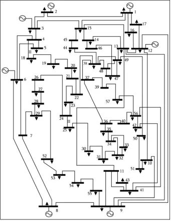
The proposed test system is IEEE57-bus system as shown in figure 1, system data are based on 100 MVA. Which consists of seven generator buses (bus 1 is slack bus 2, 3,6,8,9 and 12 are PV buses), the system has 43 loads totaling 1250.8 MW, 336.4 MVAr, real and reactive power loads, respectively. The algorithm of this method was programmed in MATLAB.
5.1. Results and Discussion
5.1.1. Base Case Results (System Without DGs)
5.1.2. System Results with DGs
In this paper, two type of DG are considered as follows: (1). Type I- DG capable of injecting real power only, like photovoltaic.
(2). Type II - DG capable of injecting both real and
reactive power, e.g. synchronous machines.To indicate and compare the effects of DGs placement in the distribution systems, different cases are considered and the results are compared to the case that there is no existence of DG in the test system. Details of cases studies are as follows:
Figure 1. 57 bus test system.
Case ‘I’: One DG installation. Case ‘II’: Two DGs installation. Case ‘III’: Three DGs installation. Case ‘IV’: Four DGs installation. Case ‘V’: Five DGs installation. Case ‘VI’six DGs installation
The size of the DG unit should not be so small or so large with relationship with the total load value. Therefore, the DG range is between 134.28 MVA (10% of total load) and 335.7 MVA (25% of total load) for this system. The results obtained in this system are briefly summarized in the following sections.
At first, run the code of (SAA) with a specific value of distributed generators (10% from total load) to determine the
best Location of distributed generators based on the power losses minimization. A minimum power loss occurs when (DG) locate at bus 13. Then, optimum size and locations of DGs for the type I for minimization of loss using SAA for all different cases are determined as shown in Table 1.
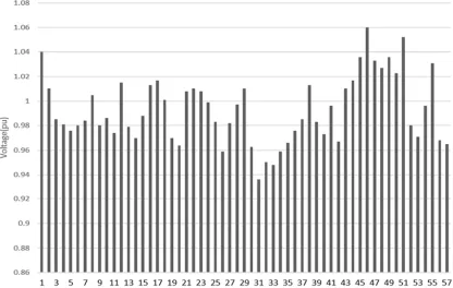
Figure 2. Voltage profile for all buses without DG.
Table 1. The Result of DGs Installation in Type I inTest System.
Method Bus. No DG Size
(MW)
DG Size (MVar)
Total DG size (MVA)
Ploss
(MW) Qloss (Mvar)
Loss reduction%
Real Reactive
Base case ---- --- ---
261.07 (20.92% FROM TOTAL LOAD)
27.864 121.67 --- ---
SA
Case I 13 261.07 0 15.9 73.17 42.93 39.86
Case II 13
36
208.89
52.17 0 14.91 67.98 46.49 44.12
Case III 13 36 55
168.35 46.7 46
0 14.76 67 47.02 44.93
Case IV 13 16 37 52
160.57 35.7 38.76 25.98
0 14.40 66.27 48.32 45.53
Case V 13 31 10 36 56
130.56 21.66 80.2 5.6 22.46
0 14.26 63 48.82 48.22
Case VI 13 30 36 54 7 55
145.0508 18.5550 20.6506 24.6861 26.2155 16.5220
0 14.7 68 47.2 44.11
Also, the voltage profile at all buses for type I is shown in figure 3, for the case V the voltage at all buses is more stable than the voltage profile for base case without DGs as shown in figure 1.
Table 2 shows the results of Optimum size, locations and numbers of DGs for the type II at all different cases which are presented in this table, the case IV is the best case compared to other cases where the five DGs with specified
increases the power loss reduction also increases but adding more than specified types of DGs to the network is not
economical considering the power loss reduction.
Table 2. The Result of DGs Installation inType IIin Test System.
Method Bus. No Dg Size
(Mw)
Dg Size (Mvar)
Total Dg
SIZE (Mva) Ploss (Mw) Qloss (Mvar)
Loss reduction%
Real Reactive
Base CASE ---- --- ---
261.07 (20.92% FROM TOTAL LOAD)
27.864 121.67 --- ---
SA
Case I 13 251.68 121.89 15.8987 73.2405 42.94 39.80
Case II 13
36
193.53 58.14
93.73
28.15 15.11 68.14 45.77 43.99
Case III
13 36 10
180 47.08 24.59
86.6 22.8 11.4
14.12 66.855 49.32 45.04
Case IV
13 16 36 54
170.48 38.42 27.007 15.76
80.44 18.6 15.2 7.63
14 66.2 49.75 45.6
Case V
13 31 10 37 28
81.8 133.6 12.14 33.1 10.8
39.6 55.1 5.8 16 5.2
14.17 65.44 49.14 46.21
Figure 3. Voltage profile for all buses with DG for type I case VI (SIX DGs).
6. Conclusion
Optimum size, location and numbers of distributed generators using Simulated Annealing Algorithm (SAA) for total loss reduction in IEEE 57-bus test system are proposed in this paper. Also, two types of DG consisting of DGs with capability of supplying real power only (type I) and DGs with capability of supplying both real power and reactive power (type II) are considered and comparative studies are conducted for different cases to investigate the impacts of DGs on total loss reduction., the outcomes uncover that the combination of DG units is highly successful in reducing power losses in the electrical network. It is possible to get the best place DG and the best size in economic terms easily in the case of the development of the study.
References
[1] A. Kazemi, and M.Sadeghi”Distributed Allocation for Loss Reduction and Voltage Improvement Generation” IEEE DOI: 10.1109 / APPEEC 4918287 Power and Energy Engineering Conference 2009.
[2] G. V. Nagesh Kumar, R. SR Krishnam Naidu, SaradaBusam,SnighaHota “Multi objective Optimization of Radial Distribution System with multiple Distributed Generation Units using Genetic Algorithm” International conference on Electrical, Electronics, Signels,Communication and Optimization (EESCO)-2015.
[3] S. Kumar Injeti, Dr.Navuri P Kumar” Optimal Planning of Distributed Generation for Improved Voltage Stability and Loss Reduction” International Journal of Computer Applications (0975 – 8887) Volume 15– No.1, February 2011. [4] Gopiya Naik. S 1, D. K. Khatod 2, M. P. Sharma “Optimal
Allocation of Distributed Generation in Distribution System for Loss Reduction” IPCSIT vol. 28 © IACSIT Press, Singapore 2012.
[5] ParthaKayal and Chandan Kumar Chanda “A simple and fast approach for allocation and size evaluation of distributed
generation” International Journal of Energy and Environmental Engineering 2013.
[6] Minnan Wang and JinZhong “A Novel Method for Distributed Generation and Capacitor Optimal Placement considering Voltage Profiles” IEEE Transactions On Power and Energy Society General Meeting, 978-1-4577-1002-5/11, 2011. [7] VahidRashtchi, Mohsen Darabian “A New BFA-Based
Approach for Optimal Sitting and Sizing of Distributed Generation in Distribution System” International Journal of Automation and Control Engineering Vol. 1 Issue 1, November 2012.
[8] Ram Singh1, Gursewak Singh Brar2 and Navdeep Kaur3 “Optimal Placement of DG in Radial Distribution Network for Minimization of Losses” International Journal of Advanced Research in Electrical, Electronics and Instrumentation Engineering Vol. 1, Issue 2, August 2012.
[9] Duong Quoc Hung, NadarajahMithulananthan, R. C. Bansal “Analytical Expressions for DG Allocation in Primary Distribution Networks” IEEE Transactions On Energy Conversion, Vol. 25, No. 3, September 2010.
[10] D. Sharma, R. Bartels, Distributed electricity generation in competitive energy markets: a case study in Australia, in: The Energy Journal Special issue: Distributed Resources: Toward a New Paradigm of the Electricity Business, The International Association for Energy Economics, Clevland, Ohio, USA, pp. 17–40,1998.
[11] CIGRE, International Council on Large Electricity Systems, http://www.cigre.org.
[12] G. Pepermans, J. Driesen, D. Haeseldonckx, R. Belmans, and W.D'Haeseleer, "Distributed generation: definition, benefits and issues", Energy Policy, vol. 33, pp. 787-798, 2005. [13] Elgerd IO. Electric energy system theory: an introduction.
New York: McGraw-Hill; 1971.
[14] Ingber, L.,, "Simulated annealing: practice versus theory", Mathl. Comput. Modelling 18, 11, 29-57, 1993.