Subgroup Analysis via Recursive Partitioning
Xiaogang Su [email protected]
Department of Statistics and Actuarial Science University of Central Florida
Orlando, FL 32816, USA
Chih-Ling Tsai [email protected]
Graduate School of Management University of California, Davis Davis, CA 95616, USA
Hansheng Wang [email protected]
Guanghua School of Management Peking University
Beijing 100871, P. R. China
David M. Nickerson [email protected]
Department of Statistics and Actuarial Science, University of Central Florida
Orlando, FL 32816, USA
Bogong Li [email protected]
Office of Survey Methods Research U.S. Bureau of Labor Statistics Washington, DC 20212, USA
Editor: Saharon Rosset
Abstract
Subgroup analysis is an integral part of comparative analysis where assessing the treatment effect on a response is of central interest. Its goal is to determine the heterogeneity of the treatment effect across subpopulations. In this paper, we adapt the idea of recursive partitioning and introduce an interaction tree (IT) procedure to conduct subgroup analysis. The IT procedure automatically facilitates a number of objectively defined subgroups, in some of which the treatment effect is found prominent while in others the treatment has a negligible or even negative effect. The standard CART (Breiman et al., 1984) methodology is inherited to construct the tree structure. Also, in order to extract factors that contribute to the heterogeneity of the treatment effect, variable importance measure is made available via random forests of the interaction trees. Both simulated experiments and analysis of census wage data are presented for illustration.
Keywords: CART, interaction, subgroup analysis, random forests
1. Introduction
to know if there are subgroups of trial participants who are more (or less) likely to be helped (or harmed) by the intervention under investigation. Subgroup analysis helps explore the heterogeneity of the treatment effect and extract the maximum amount of information from the available data. According to a survey conducted by Assmann et al. (2000), 70% of trials published over a three-month period in four leading medical journals involved subgroup analyses.
The research questions in subgroup analysis can be either pre-planned or raised in a post-hoc manner. If there is a prior hypothesis of the treatment effect being different in particular subgroups, then this hypothesis and its assessment should be part of the planned study design (CPMP, 1995). At the same time, subgroup analysis is also often used for post-hoc exploratory identification of unusual or unexpected results (Chow and Liu, 2004). Suppose, for example, that it is of interest to investigate whether the treatment effect is consistent among three age groups: young, middle-aged, and older individuals. The evaluation is formally approached by means of an interaction test between treatment and age. If the resulting test is significant, multiple comparisons are then used to find out further details about the magnitude and direction of the treatment effect within each age group. To ensure a valid experimentwise false positive rate, adjustment methods such as Bonferroni typed correction are often applied.
Limitations of traditional subgroup analysis have been extensively noted (see, e.g., Assmann et al., 2000, Sleight, 2000, and Lagakos, 2006). First of all, the subgroups themselves, as well as the number of subgroups to be examined, are specified by the investigator beforehand in the current practice of subgroup analysis, which renders subgroup analysis a highly subjective process. Even for the field expert, it is a daunting task to determine which specific subgroups should be used in subgroup analysis. The subjectivity may lead directly to dubious results and willful manipulations. For example, one may fail to identify a subgroup of great prospective interest or intentionally avoid reporting subgroups where the investigational treatment is found unsuccessful or even potentially harmful. Reliance on such analyses is likely to be erroneous and harmful. Moreover, significance testing is the main approach in subgroup analysis. Because there is no general guideline for se-lecting the number of subgroups, one has to examine numerous plausible possibilities to have a thorough assessment of the treatment effect. However, a large number of subgroups inevitably causes concerns related to multiplicity and lack of power.
In this paper, we propose a data-driven tree procedure, labelled as “interaction trees” (IT), to explore the heterogeneity structure of the treatment effect across a number of subgroups that are objectively defined in a post hoc manner. The tree method, also called recursive partitioning, was first proposed by Morgan and Sonquist (1963). By recursively bisecting the predictor space, the hi-erarchical tree structure partitions the data into meaningful groups and makes available a piecewise approximation of the underlying relationship between the response and its associated predictors. The applications of tree models have been greatly advanced in various fields especially since the development of CART (classification and regression trees) by Breiman et al. (1984). Their pruning idea for tree size selection has become and remains the current standard in constructing tree models.
2. Tree-Structured Subgroup Analysis
We consider a study designed to assess a binary treatment effect on a continuous response or output while adjusting or controlling for a number of covariates. Suppose that the data available contain n i.i.d. observations{(yi,trti,xi): i=1, . . . ,n},where yi is the continuous response; trtiis the binary
treatment indicator taking values 1 or 0; and xi= (xi1, . . . ,xip)0 is the associated p-dimensional
covariate vector where its components can be of mixed types, that is, categorical or continuous. Our goal in subgroup analysis is to find out whether there exist subgroups of individuals in which the treatment shows heterogeneous effects, and if so, how the treatment effect varies across them.
Applying a tree procedure to guide the subgroup analysis is rather intuitive. First, subgroup analysis essentially involves the interaction between the treatment and the covariates. The tree algorithm is known as an excellent tool for exploring interactions. As a matter of fact, the first im-plementation of decision trees is referred to as Automatic Interaction Detection (AID; Morgan and Sonquist, 1963). However, tree methods handle interactions implicitly. It is often hard to determine whether or not interaction really exists among variables for a given tree structure. We shall seeks ways that enable us to explicitly assess the interaction between the treatment and the covariates. Secondly, the hierarchical binary tree structure naturally groups data in an optimal way. By recur-sively partitioning the data into two subgroups that show the greatest heterogeneity in treatment effect, we are able to optimize the subgroup analysis and make it more efficient in representing the heterogeneity structure of the treatment effect. Thirdly, the tree procedure is objective, data-driven, and automated. The grouping strategy and the number of subgroups are automatically determined by the procedure. The proposed method would result in a set of objectively recognized and mutu-ally exclusive subgroups, ranking from the most effective to the least effective in terms of treatment effect. To the best of our knowledge, Negassa et al. (2005) and Su et al. (2008), who studied tree-structured subgroup analysis in the context of censored survival data, are the only previous works along similar lines to our proposal.
To construct the IT model, we follow the CART (Breiman et al., 1984) convention, which consists of three major steps: (1) growing a large initial tree; (2) a pruning algorithm; and (3) a validation method for determining the best tree size. Once a final tree structure is obtained, the subgroups are naturally induced by its terminal nodes. To achieve better efficiency, an amalgamation algorithm is used to merge terminal nodes that show homogenous treatment effects. In addition, we adopt the variable importance technique in the context of random forest to extract covariates that exhibit important interactions with the treatment.
2.1 Growing a Large Initial Tree
We start with a single split, say s, of the data. This split is induced by a threshold on a predictor X . If X is continuous, then the binary question whether X≤c is considered. Observations answering “yes” go to the left child node tLand observations answering “no” go to the right child node tR.
If X is nominal with r distinct categories C={c1, . . . ,cr}, then the binary question becomes “Is
X ∈A?” for any subset A⊂C. When X has many distinct categories, one may place them into
order according to the treatment effect estimate within each category and then proceed as if X is ordinal. This strategy helps reduce the computational burden. A theoretical justification is provided by Theorem 1 in the appendix.
child node
treatment tL tR
1 µL1 y¯L1 s21 n1 µR1 y¯R1 s22 n2 0 µL0 y¯L0 s23 n3 µR0 y¯R0 s24 n4
Here,{µL1,y¯1L,s21,n1}are the population mean, the sample mean, the sample variance, and the sample size for the treatment 1 group in the left child node tL, respectively. Similar notation applies to the
other quantities. To evaluate the heterogeneity of the treatment effect between tLand tR, we compare
(µL
1−µL0)with(µR1−µR0)so that the interaction between split s and treatment is under investigation. A natural measure for assessing the interaction is given by
t(s) = (y¯
L
1−y¯L0)−(y¯R1−y¯R0) ˆ
σ·p1/n1+1/n2+1/n3+1/n4, (1)
where ˆσ2=∑4i=1wis2i is a pooled estimator of the constant variance, and wi= (ni−1)/∑4j=1(nj−
1). For a given split s, G(s) =t2(s) converges to aχ2(1) distribution. We will use G(s) as the splitting statistic, while remaining aware that the sign of t(s)supplies useful information regarding the direction of the comparison.
The best split s? is the one that yields the maximum G statistic among all permissible splits. That is,
G(s?) =max
s G(s).
The data in node t are then split according to the best split s?. The same procedure is applied to split both child nodes: tLand tR. Recursively doing so results in a large initial tree, denoted by T0.
Remark 1: It can be easily seen that t(s)given in (1) is equivalent to the t test for testing H0:γ=0 in the following threshold model
yi=β0+β1·trti+δ·zi(s)+γ·trti·z(is)+εi, (2)
where z(is)=1{Xi≤c}is the binary variable associated with split s. This observation sheds light on ex-tensions of the proposed method to situations involving different types of responses and multi-level treatments. Note that inclusion of both trti and z(is) in model (2) is important to assure the
corre-spondence between the regression coefficientγand the interaction, that is,γ= (µL
1−µL0)−(µR1−µR0).
Remark 2: In constructing the large initial tree T0, a terminal node is declared when any one of
2.2 Pruning
The final tree could be any subtree of T0. To narrow down the choices, Breiman et al. (1984) proposed a pruning algorithm which results in a sequence of optimally pruned subtrees by iteratively truncating the “weakest link” of T0. In the following, we briefly describe an interaction-complexity pruning procedure, which is analogous to the split-complexity pruning algorithm in LeBlanc and Crowley (1993). We refer the reader to their paper for a detailed description.
To evaluate the performance of an interaction tree T , we define an interaction-complexity mea-sure:
Gλ(T) =G(T)−λ· |T−Te|, (3)
where G(T) =∑h∈T−TeG(h)measures the overall amount of interaction in T ; the total number of internal nodes |T−Te|corresponds to the complexity of the tree; and the complexity parameter λ≥0 acts as a penalty for each added split. Given a fixedλ, a tree with larger Gλ(T)is preferable. Start with T0. For any internal node h of T0, calculate g(h) =G(Th)/|Th−Teh |, where Th
is the branch with h as root and|Th−Teh|denotes the number of internal nodes of Th. Then, the
node h? with smallest g(h?)is the “weakest link,” in the sense that h? becomes ineffective first as λincreases. Next, let T1be the subtree after pruning off the branch Th? from T0,and subsequently apply the same procedure to prune T1. Repeating this procedure yields a nested sequence of subtrees TM≺ ··· ≺Tm≺Tm−1≺ ··· ≺T1≺T0, where TMis the null tree with the root node only and≺means
“is a subtree of”.
2.3 Selecting the Best-Sized Subtree
The final tree will be selected from the nested subtree sequence{Tm: m=0,1, . . . ,M}, again, based
on the maximum interaction-complexity measure Gλ(Tm)given in (3). For tree size determination
purposes, λ is suggested to be fixed within the range 2≤λ≤4, where λ=2 is in the spirit of the Akaike information criterion (AIC; Akaike, 1973) andλ=4 corresponds roughly to the 0.05 significance level on theχ2(1)curve. Another choice isλ=ln(n), citing the Bayesian information criterion (BIC; Schwarz, 1978).
To overcome the over-optimism due to greedy search, an “honest” estimate of the goodness-of-split measure G(Tm) is needed. This can be achieved by a validation method. If the sample size
is large, G(Tm)can be recalculated using an independent subset of the data (termed the validation
sample). If the sample size is small or moderate, one has to resort to techniques such as v-fold cross-validation or bootstrapping methods in order to validate G(Tm). The bootstrap method used
in LeBlanc and Crowley (1993), for example, can be readily adapted to interaction trees.
Remark 3: As another alternative, one referee suggested the use of in-sample BIC to determine
the optimally-sized subtree, which can be promising, although further research effort is needed to determine the effective degrees of freedom (see, e.g., Ye, 1998, and Tibshirani and Knight, 1999) associated with interaction trees.
2.4 Summarizing the Terminal Nodes
con-ventional subgroup analysis, the subgroups obtained from the IT procedure are mutually exclusive. Due to the subjectivity in determining the subgroups and multiplicity emerging from significance testings across subgroups, it is generally agreed that subgroup analysis should be regarded as ex-ploratory and hypothesis-generating. As recommended by Lagakos (2006), it is best not to present p-values for within-subgroup comparisons, but rather to give an estimate of the magnitude of the treatment difference. To summarize the terminal nodes, one can compute the average responses for both treatments within each terminal node, as well as their relative differences or ratios and the associated standard errors. If, however, one would like to perform some formal statistical testings, then it is important to conduct these tests based on yet another independent sample. To do so, one partitions the data into three sets: the learning sample
L
1, the validation sampleL
2, and the test sampleL
3. The best IT structure will be developed usingL
1 andL
2,and then reconfirmed using the test sampleL
3.It happens often that the treatment shows homogeneous effects for entirely different causal rea-sons in terminal nodes stemming from different branches. In this case, a merging scheme analogous to the approach of Ciampi et al. (1986) can be useful to further bring down the number of final sub-groups. A smaller number of subgroups are easier to summarize and comprehend and more efficient to represent the heterogeneity structure for the treatment effect. It also ameliorates the multiplicity issue in within-subgroup comparisons. In this scheme, one computes the t statistic in equation (1) between every pair of the terminal nodes. The pair showing the least heterogeneity in treatment effect are then merged together. The same procedure is executed iteratively until all the remaining subgroups display outstanding heterogeneity. In the end, one can sort the final subgroups based on the strength of the treatment effect, from the most effective to the least effective.
Remark 4: The hierarchical tree structure is appealing mainly because of its easy interpretability.
Apparently the merging scheme would invalidate the tree structure, yet lead to better interpretations. It is noteworthy that this merging scheme contributes additional optimism to the results. Thus, we suggest that amalgamation be executed with data(
L
1+L
2)that pool the learning sampleL
1and the validation sampleL
2together, so that the resultant subgroups can be validated using the test sampleL
3.We shall illustrate this scheme with an example presented in Section 4.2.5 Variable Importance Measure via Random Forests
Algorithm 1: Computing Variable Importance Measure via Random Forests.
Initialize all Vj’s to 0.
For b=1,2, . . . ,B,do
•Generate bootstrap sample
L
band obtain the out-of-bag sampleL
−L
b. •Based onL
b, grow a large IT tree Tbby searching over m0randomly selectedcovariates at each split.
•Send
L
−L
bdown Tbto compute G(Tb). •For all covariates Xj, j=1, . . . ,p, do◦Permute the values of Xjin
L
−L
b.◦Send the permuted
L
−L
bdown to Tbto compute Gj(Tb). ◦Update Vj←Vj+G(TbG(T)−Gj(Tb)b) .
•End do.
End do.
Average Vj←Vj/B.
Let Vj denote the importance measure of the j-th covariate or feature Xj for j=1, . . . ,p.We
construct random forests of IT trees by taking B bootstrap samples
L
b, b=1, . . . ,B.This is doneby searching over only a subset of randomly selected m0covariates at each split. For each IT tree Tb, the b-th out-of-bag sample (denoted as
L
−L
b), which contains all observations that are notin
L
b, is sent down Tb to compute the interaction measure G(Tb). Next, the values of the j-thcovariate in
L
−L
bare randomly permuted. The permuted out-of-bag sample is then sent down Tbto recompute Gj(Tb). The relative difference between G(Tb)and Gj(Tb)is recorded. The procedure
is repeated for B bootstrap samples. As a result, the importance measure Vj is the average of the
relative differences over all B bootstrap samples. The whole procedure is summarized in Algorithm 1.
The variable importance technique in random forests has been increasingly studied in its own right and applied as a tool for variable selection in various fields. This method generally belongs to the “cost-of-exclusion” (Kononenko and Hong, 1997) feature selection category, in which the importance or relevance of a feature is determined by the difference in some model performance measure with and without the given feature included in the modeling process. In Algorithm 1, random forests make available a flexible modeling process while exclusion of a given feature is carried out by permutating its values.
3. Simulated Studies
Error
Model Form Distribution
A Y =2+2·trt+2 Z1+2 Z2+ε
N
(0,1) B Y =2+2·trt+2 Z1+2 Z2+2·trt·Z1Z2+εN
(0,1) C Y =2+2·trt+2 Z1+2 Z2+2·trt·Z1+2·trt·Z2+εN
(0,1) D Y =10+10·trt·exp{(X1−0.5)2+ (X2−0.5)2}+εN
(0,1) E Y =2+2·trt+2 Z1+2 Z2+2·trt·Z1+2·trt·Z2+ε Unif(−√
3,√3) F Y =2+2·trt+2 Z1+2 Z2+2·trt·Z1+2·trt·Z2+ε exp(1)
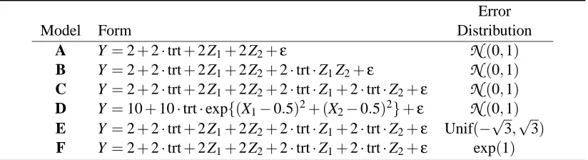
Table 1: Models used for assessing the performance of the IT procedure. Note that Z1=1{X1≤0.5} and Z2=1{X2≤0.5}.
Specifically, Model A is a plain additive model with no interaction. It helps assess the type I error or false positive rate when using the IT procedure. Model B involves a second-order interaction between the treatment and two terms of thresholds, both at 0.5, on X1and X2. If the IT procedure works, a tree structure with three terminal nodes should be selected. In Model C, the two thresholds, each interacting with the treatment, are present in an additive manner. Model D involves interaction of complex forms other than cross-products. A large tree is expected in order to represent the interaction structure in this case. Models E and F are similar to Model C, but with different error distributions. They are useful in evaluating the robustness of the IT procedure to deviations from normality.
Only one set of sample sizes is reported: 800 observations in the learning sample
L
1 and 400 observations in the validation sampleL
2.Each model is examined for 200 simulation runs and four choices ofλ,{2,3,4,ln(400)}, are considered for determining the best tree structure. The relative frequencies of the final tree sizes selected by the IT procedure are presented in Table 2. The expected final tree size for each model is highlighted in boldface. Note that both X1 and X2, but neither X3 nor X4, are actually involved in models B-F. To address the variable selection issue, we count the frequency of “hits” (i.e., the final tree selected by the IT procedure is split by X1and X2and only by them). The results are presented in the last column of Table 2.We first examine the results for Model A, which involves no interaction. The IT procedure correctly selects the null tree structure at least 83.5% of the time. Whenλ=ln(n), the percentage of correct selections becomes 98.5%. The 98.5% of correct selections yields an empirical size of 100%-98.5% = 1.5%, which is well within the acceptable level. This implies that the chance for the IT procedure to extract an unsolicited interactions is really small. For models B-F, the IT procedure also successfully identifies the true final tree structure and selects the desired splitting variables a majority of the time. Moreover, from results for models E and F, it seems rather robust against deviations from normality. When comparing different complexity parameters, we see thatλ=ln(n) provides the best selection. This is mainly because of the large sample size and relatively strong signals considered in our simulation configuration (see, e.g., McQuarrie and Tsai, 1998).
Complexity Final Tree Size
Model λ 1 2 3 4 5 6 ≥7 Hits
A 2 83.5 5.0 2.5 2.5 2.0 0.5 4.0 83.5
3 94.0 3.5 0.5 0.5 1.0 0.5 0.0 94.0
4 97.5 2.5 0.0 0.0 0.0 0.0 0.0 97.5
ln(n) 98.5 1.5 0.0 0.0 0.0 0.0 0.0 98.5
B 2 0.0 0.0 67.0 9.0 9.0 2.5 12.5 77.5
3 0.0 0.0 83.0 6.5 5.5 1.0 4.0 90.0
4 0.0 0.0 89.0 6.5 3.0 1.0 0.5 95.0
ln(n) 1.0 0.0 91.5 6.5 2.0 0.0 0.0 97.5
C 2 0.0 0.0 0.0 66.5 10.5 9.5 13.5 77.5
3 0.0 0.0 0.0 82.5 7.5 6.0 4.0 90.5
4 0.0 0.0 0.0 88.0 6.5 4.5 1.0 95.0
ln(n) 0.0 0.0 0.0 94.0 4.0 1.5 0.5 98.5
D 2 0.0 0.0 0.0 0.0 13.0 10.5 76.5 66.5
3 0.0 0.0 0.0 0.5 24.5 16.0 59.0 83.5 4 0.0 0.0 0.0 0.5 35.5 18.5 45.5 91.5 ln(n) 0.0 0.0 2.0 3.5 54.0 16.0 24.5 96.0
E 2 0.0 0.0 0.0 74.0 12.0 6.0 8.0 82.0
3 0.0 0.0 0.0 88.5 7.5 3.5 0.5 93.0
4 0.0 0.0 0.0 93.5 5.0 1.0 0.5 97.5
ln(n) 0.0 0.0 0.0 97.0 2.5 0.0 0.5 98.5
F 2 0.0 0.0 0.0 67.5 13.0 8.0 11.5 76.5
3 0.0 0.0 0.0 84.5 7.0 4.5 4.0 91.0
4 0.0 0.0 0.0 90.0 7.5 1.5 1.0 96.5
ln(n) 0.0 0.0 0.0 95.0 4.5 0.5 0.0 99.0
Table 2: Relative frequencies (in percentages) of the final tree size identified by the interaction tree (IT) procedure in 200 runs.
−0.09
−0.06
−0.03
Model A − I
importance
X1 X2 X3 X4
0.1
0.3
Model A − II
logworth
X1 X2 X3 X4
0.0
0.1
0.2
0.3
Model B − I
importance
X1 X2 X3 X4
0.0
1.0
2.0
3.0
Model B − II
logworth
X1 X2 X3 X4
0.0
0.2
0.4
Model C − I
importance
X1 X2 X3 X4
0
5
10
15
Model C − II
logworth
X1 X2 X3 X4
0.0
0.1
0.2
0.3
Model D − I
importance
X1 X2 X3 X4
0.2
0.6
Model D − II
logworth
X1 X2 X3 X4
0.0
0.2
0.4
Model E − I
importance
X1 X2 X3 X4
0
2
4
6
8
Model E − II
logworth
X1 X2 X3 X4
0.0
0.2
0.4
Model F − I
importance
X1 X2 X3 X4
0 2 4 6 8 12
Model F − II
logworth
X1 X2 X3 X4
Figure 1: Variable Importance via Random Forests and Feature Selection for the Six Simulation Models. With a data set consisting of 1200 observations generated from Model A, Graph A-I plots the variable importance score computed from 500 random interaction trees while Graph A-II plots the logworth of the p-value from the simple feature selection method. Note that logworth =−log10(p-value). Similar methods were used to make other graphs.
and mistakenly selects X4.In Figure D-II, none of the covariates are found important.
Name Type Levels Description
X1 age continuous 70 age
X2 workclass categorical 4 class of worker
X3 education ordinal 16 education levels
X4 marital categorical 7 marital status
X5 industry1 categorical 22 major industry
X6 occupation2 categorical 13 major occupation
X7 race categorical 5 race
X8 union categorical 2 member of a labor union
X9 fulltime categorical 6 full or part time employment
X10 tax.status categorical 6 tax filer status
X11 household.sum3 categorical 7 detailed household summary
X12 n.emplyee ordinal 7 number of persons worked for employer
X13 country.birth categorical 39 country of birth
X14 citizenship categorical 7 US citizen or not
X15 self.employed categorical 3 own business or self employed X16 weeks.worked continuous 53 weeks worked in year
1The specific levels for industry (X
5): 1 Agriculture; 2 Business and repair services; 3
-Communications; 4 - Construction; 5 - Education; 6 - Entertainment; 7 - Finance insurance and real estate; 8 Forestry and fisheries; 9 Hospital services; 10 Manufacturingdurable goods; 11 -Manufacturing-nondurable goods; 12 - Medical except hospital; 13 - Mining; 14 - Other professional services; 15 - Personal services except private HH; 16 - Private household services; 17 - Public administration; 19 - Retail trade; Social services; 20 - Transportation; 21 - Utilities and sanitary services; 22 - Wholesale trade.
2The specific levels foroccupation(X
6): 1- Adm support including clerical; 2 - Executive admin
and managerial; 3 - Farming forestry and fishing; 4 - Handlers equip cleaners etc; 5 - Machine operators assmblrs & inspctrs; 6 - Other service; 7 - Precision production craft & repair; 8 - Private household services; 9 - Professional specialty; 10 - Protective services; 11 - Sales; 12 - Technicians and related support; 13 - Transportation and material moving.
3The specific levels for household.sum(X
11): 1 - Child 18 or older; 2 - Child under 18 never
married; 3 - Group Quarters, Secondary individual; 4 - Householder; 5 - Nonrelative of householder; 6 - Other relative of householder; 7 - Spouse of householder.
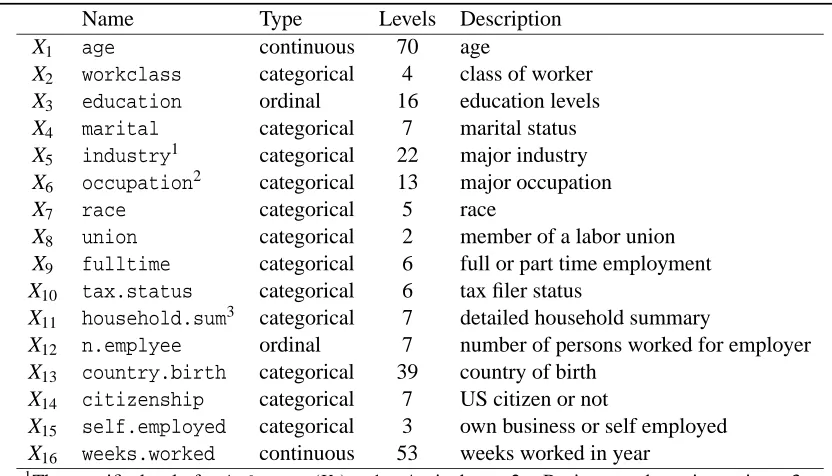
Table 3: Variable Description for the Census Wage Data.
4. An Example - The CPS Data
0 5 10 15 20 25 30 35
0
50
100
150
200
number of terminal nodes
23 G(2)
10
G(3) 9
G(4) 9
G(ln(n))
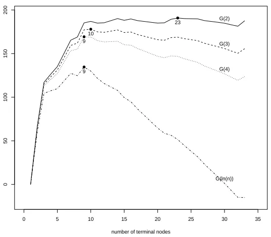
Figure 2: Tree size selection for the CPS data (the plot of Gλ(Tm)vs. tree size).
The quest becomes complicated when there are a large number of classification variables to choose from, which motivates the IT procedure.
We extract data from the Current Population Survey (CPS) database, which can be accessed at (http://www.census.gov/cps/). The CPS is a national monthly survey of approximately 60,000 households conducted by the U.S. Census Bureau for the Bureau of Labor Statistics. Information collected in the survey includes employment status, hours worked and income from work as well as a number of demographic characteristics of the household members. From the CPS 1995 March Supplement, we compile a data set, which contains 16,602 individuals with no missing value in-volved. We use hourly wages in U.S. dollars as a measure of pay. Besides gender, there are a total of 16 demographical covariates included. A brief description for these covariates is given in Table 3. Several of them are nominal with many levels. We only list detailed codings for those variables appearing in the final tree structure.
To apply IT, we take a logarithmic transformation on wage. Then, we randomly divide the entire data (denoted as
L
) into three sets with a ratio of approximately 2: 1: 1. A large initial tree with 33 terminal nodes is constructed and pruned using data inL
1. Sending the validation sampleL
2down each subtree, Figure 2 depicts the resultant Gλ(Tm) score versus the subtree size. It can19.81 X5∈ {1,6,8,9} IV 1,550 0.802 @ @@
16.34 X11∈ {4}
5.52 X1≤42
−12.24 X6∈ {3,8,13}
I 252 1.612 ,, , l ll
6.98 X6∈ {/ 1,5,7,11}
8.99 X5∈ {/ 10,11,18}
III 1,395 0.883 T TT II 1,189 1.116 @ @@ II 3,170 1.150 @ @@ II 1,896 1.361 HH HHH
14.79 X5∈ {/ 3,4,10,11,14,15,17,18,20}
II 2,052 1.208 ,, , l ll
13.83 X6∈ {2,3,8,10,13}
II 819 1.078 T TT I 4,279 1.509
Figure 3: The best-sized interaction tree for the CPS data selected by BIC. For each internal node denoted by a box, the splitting rule is given inside the box. Observations satisfying the condition go to the left node while observations not satisfying the condition go the right node. To the left of each internal node is the t(s) test statistic recomputed using
L
3. Terminal nodes are denoted by circles and ranked with Roman numerals on the left. The node size (i.e., number of individuals) is given inside the circle and the ratio of average wages for males versus females is given underneath, both based on the entire data setL
.I, women are most underpaid compared to men. In Group II, women are somewhat underpaid, etc. This specification was also made available to each terminal node in Figure 3.
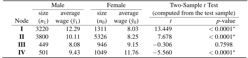
Table 4 summarizes the final four subgroups. For each subgroup, the number of men and women, as well as their average wages, are computed based on the whole data
L
.The two-sample t test for comparing the average wages between men and women is also presented. This test was computed by using the test sampleL
3. Since there are four tests performed, one may compare the resultant p-values with 0.05/4=0.0125 by applying the Bonferroni-typed adjustment to the joint significant levelα=0.05.As a result, Groups I, II, and IV, each marked with an asterisk, show significant differences in wage between men and women.0.00
0.05
0.10
0.15
0.20
(a)
covariate
importance
1 2 3 4 5 6 7 8 9 10 11 12 13 14 15 16
0
5
10
15
20
25
(b)
covariate
logworth
1 2 3 4 5 6 7 8 9 10 11 12 13 14 15 16
Figure 4: Variable importance measures for the CPS Data: (a), via random forests of interaction trees; (b), based on the p-value associated with the interaction terms in an interaction model that includes the treatment and the covariate only. Note that the logworth is
−log10(p-value).The sixteen covariates areage(X1),workclass(X2),education(X3),
marital(X4),industry(X5),occupation(X6),race(X7),union(X8),fulltime(X9),
tax.status (X10), household.sum (X11), n.employee (X12), country.birth (X13),
citizenship(X14),self.employed(X15), andweeks.worked(X16).
hour while the average wage of women is only $8.03 per hour. Interestingly the IT tree has also identified a subgroup, Group IV, in which men are underpaid compared to women. This occurs in the following industries (X5): 1 Agriculture; 6 Entertainment; 8 Forestry and fisheries; 9 -Hospital services.
Male Female Two-Sample t Test size average size average (computed from the test sample) Node (n1) wage ( ¯y1) (n0) wage ( ¯y0) t p-value
I 3220 12.29 1311 8.03 13.449 <0.0001?
II 3800 10.11 5326 8.25 7.678 <0.0001?
III 449 8.08 946 9.15 −0.306 0.7598
IV 501 9.43 1049 11.76 −5.560 <0.0001?
Table 4: Summary statistics for the four final subgroups of the CPS data. Note that(n1,y1¯ ,n0,y0)¯ are computed using the whole data. The two-sample t test statistics are calculated from the test sample
L
3. The associated p-values are obtained for two-sided tests.(X4) have been masked out. The simple feature selection technique is also used to determine the importance of each covariate. Figure 4(b) depicts the resulting logworths. While both plots show some similarities, one should keep in mind that evaluation based on the latter approach is rather restrictive.
5. Discussion
In data analysis, it is important to distinguish two types of interactions. If there is no directional change in terms of the comparison, that is,(µL
1−µL0)·(µR1−µR0)>0, the interaction is said to be quantitative; otherwise, it is termed as qualitative. The presence of qualitative interactions causes more concerns than quantitative ones (see, e.g., Gail and Simon, 1985). The results from the IT procedure can help to address this issue. For instance, the qualitative interaction in the the CPS example is obviously present among the final four subgroups.
The proposed IT procedure is applicable to a number of different areas. For example, the IT structure can help identify the most and least effective subgroups for the investigational medicine. If the new medicine shows an overall effect that is significant, and, if even in the least effective subgroup under examination, it does not present any harmful side effects, then its release may be endorsed without reservation. In trials where the proposed compound is not found to be significantly effective, the tree-structured subgroup analysis may identify sub-populations that contribute to the failure of the compound. Information gained in this manner could provide the basis for establish-ing inclusion/exclusion criteria in future trials, and as such, could be of considerable value to the existing efforts in synthesizing compounds to fight deadly diseases such as cancer and HIV/AIDS. We believe that efforts along these lines make subgroup analysis an efficient and valuable tool for research in many application fields.
Acknowledgments
Appendix A. Categorical Splits
The following theorem provides motivation and justification for the computationally efficient strat-egy of “ordinalizing” categorical covariates in interaction trees as discussed in Section 2.1. It is analogous to Theorem 9.6 of CART (Breiman et al., 1984, pp. 274–278) yet makes a stronger statement.
Consider splits based on a categorical covariate X , whose possible values range over a finite set C={c1, . . . ,cr}.Then any subset A⊂C, together with its complement A0=C−A, induces a
partition of the data into tL={(yi,trti,xi): xil∈A}and tR={(yi,trti,xi): xil∈A0}.In the setting
of interaction trees, the splitting rule seeks an optimal partition (A+A0) to maximize the differ-ence in treatment effect between two child nodes (µL
1−µL0)−(µR1−µR0) 2
, where µL1 =µA1 =
E(y|xil∈A,trti=1) denotes the treatment mean in the left child node, and a similar definition
applies for the other µ’s. For the sake of convenience, we assume(µL
1−µL0)>(µR1−µR0)so that an optimal split maximizes(µL
1−µL0)−(µR1−µR0).
Theorem 1. Let µck=E(y|X=c,trt=k)for any element c∈C and k=0,1.If(A+A0)forms
an optimal partition of C, then we have
µc11−µc10 ≥ µc21−µc20, for any element c1∈A and c2∈A0.
Proof. Define
d1=min
c∈A(µc1−µc0) and d2=maxc∈A0(µc1−µc0).
Accordingly, it suffices to show that d1≥d2. To proceed, let
A1 = {c∈A : µc1−µc0=d1}
A2 =
c∈A0: µc1−µc0=d2 A3 = {c∈A : µc1−µc0>d1}
A4 = c∈A0: µc1−µc0<d2 .
Thus A=A1+A3 and A0 =A2+A4.We reserve a generic notation d=µ1−µ0 for the treatment effect. Define
di =
∑
c∈Ai
(µc1−µc0)Pr{Xj=c},
di j =
∑
c∈Ai∪Aj
(µc1−µc0)Pr{Xj=c},
di jk =
∑
c∈Ai∪Aj∪Ak
(µc1−µc0)Pr{Xj=c}.
for i6= j6=k=1,2,3,4.We also introduce notation Qi=Pr{Xj∈Ai}for i=1,2,3,4.It can be
verified that
di j=
diQi+djQj
Qi j
and
di jk=
diQi+djQj+dkQk
Qi jk
with Qi jk=Qi+Qj+Qk.
Since partition (A+A0) provides an optimal partition, d13−d24 >0 reaches the maximum among all possible partitions. In particular, for partition(A3+A03), we have d13−d24≥d3−d124, which can be shown equivalent to
d1≥(1−Q3)d13+Q3d24, (4)
by first plugging in the following two relationships
d3 =
Q13d13−Q1d1 Q3
d124 = Q24d24+d1Q1
Q124
and then simplifying. Similarly, for partition(A0
4+A4), we can establish
Q4d13+ (1−Q4)d24≥d2 (5)
starting with d13−d24≥d123−d4.
Now suppose that d2≥d1.It follows from (5) and (4) that
Q4d13+ (1−Q4)d24≥d2≥d1≥(1−Q3)d13+Q3d24
=⇒ {Q4d13+ (1−Q4)d24} − {(1−Q3)d13+Q3d24} ≥ d2−d1
=⇒ Q12(d24−d13) ≥ d2−d1, since 1−Q3−Q4=Q1+Q2=Q12.
However, 0>d24−d13leads to 0>d2−d1,which contradicts the condition d1≤d2.Thus we must have d1>d2.
The theorem also holds in extreme cases such as d1=d3or d2=d4, etc. The proofs are omitted.
References
H. Akaike. Information theory and an extension of the maximum likelihood principle. In B. N. Petrov and F. Czaki, editors, 2nd Int. Symp. Inf. Theory, pages 267–281. Budapest: Akad Kiado, 1973.
S. F. Assmann, S. J. Pocock, L. E. Enos, and L. E. Kasten. Subgroup analysis and other (mis)uses of baseline data in clinical trials. Lancet, 255:1064–1069, 2000.
L. Breiman. Random forests. Machine Learning, 45:5–32, 2001.
L. Breiman, J. Friedman, R. Olshen, and C. Stone. Classification And Regression Trees. Wadsworth International Group, Belmont, CA, 1984.
A. Ciampi, J. Thiffault, J.-P. Nakache, and B. Asselain. Stratification by stepwise regression, corre-spondence analysis and recursive partition. Computational Statistics and Data Analysis, 4:185– 204, 1986.
CPMP Working Party on Efficacy on Medicinal Products. Biostatistical methodology in clinical trials in applications for marketing authorisations for medicinal products: Note for guidance. Statistics in Medicine, 14:1659–1682, 1995.
M. Gail and R. Simon. Testing for qualitative interactions between treatment effects and patient subsets. Biometrics, 41:362–372, 1985.
I. Kononenko and S. J. Hong. Attribute Selection for Modeling. In: Future Generation Computer Systems, 13:181–195, 1997.
S. W. Lagakos. The challenge of subgroup analyses - reporting without distorting. The New England Journal of Medicine, 354:1667–1669, 2006.
M. Leblanc and J. Crowley. Survival trees by goodness of split. Journal of the American Statistical Association, 88:457–467, 1993
A. D. R. McQuarrie and C.-L. Tsai. Regression and Time Series Model Selection. Singapore: World Scientific, 1998.
J. Morgan and J. Sonquist. Problems in the analysis of survey data and a proposal. Journal of the American Statistical Association, 58:415–434, 1963.
A. Negassa, A. Ciampi, M. Abrahamowicz, S. Shapiro, and J.-F. Boivin. Tree-structured subgroup analysis for censored survival data: validation of computationally inexpensive model selection criteria. Statistics and Computing, 15:231–239, 2005.
G. Schwarz. Estimating the dimension of a model. Annals of Statistics, 6:461–464, 1978.
P. Sleight. Debate: Subgroup analyses in clinical trials: Fun to look at, but don’t believe them! Current Controlled Trials on Cardiovascular Medicine, 1:25–27, 2000.
X. G. Su, T. Zhou, X. Yan, J. Fan, and S. Yang. Interaction trees with censored survival data. The International Journal of Biostatistics, vol. 4 : Iss. 1, Article 2, 2008. Available at:
http://www.bepress.com/ijb/vol4/iss1/2.
R. Tibshirani and K. Knight. The covariance inflation criterion for adaptive model selection. Journal of the Royal Statistical Society, Series B, 61:529–546, 1999.
L. Torgo. A study on end-cut preference in least squares regression trees. Proceedings of the 10th Portuguese Conference on Artificial Intelligence. Lecture Notes In Computer Science, 2258:104– 115. Springer-Verlag: London, UK, 2001.