Random Walk Kernels and Learning Curves for Gaussian Process Regression on Random Graphs

Random Walk Kernels and Learning Curves for Gaussian Process

Regression on Random Graphs

Matthew J. Urry [email protected]

Peter Sollich [email protected]

Department of Mathematics King’s College London London, WC2R 2LS, U.K.

Editor:Manfred Opper

Abstract

We consider learning on graphs, guided by kernels that encode similarity between vertices. Our fo-cus is on random walk kernels, the analogues of squared exponential kernels in Euclidean spaces. We show that on large, locally treelike graphs these have some counter-intuitive properties, specif-ically in the limit of large kernel lengthscales. We consider using these kernels as covariance func-tions of Gaussian processes. In this situation one typically scales the prior globally to normalise the average of the prior variance across vertices. We demonstrate that, in contrast to the Euclidean case, this generically leads to significant variation in the prior variance across vertices, which is undesir-able from a probabilistic modelling point of view. We suggest the random walk kernel should be normalised locally, so that each vertex has the same prior variance, and analyse the consequences of this by studying learning curves for Gaussian process regression. Numerical calculations as well as novel theoretical predictions for the learning curves using belief propagation show that one obtains distinctly different probabilistic models depending on the choice of normalisation. Our method for predicting the learning curves using belief propagation is significantly more accurate than previous approximations and should become exact in the limit of large random graphs.

Keywords: Gaussian process, generalisation error, learning curve, cavity method, belief propaga-tion, graph, random walk kernel

1. Introduction

Gaussian processes (GPs)have become a workhorse for probabilistic inference that has been de-veloped in a wide range of research fields under various guises (see for example Kleijnen, 2009; Handcock and Stein, 1993; Neal, 1996; Meinhold and Singpurwalla, 1983). Their success and wide adoption can be attributed mainly to their intuitive nature and ease of use. They owe their intu-itiveness to being one of a large family of kernel methods that implicitly map lower dimensional spaces with non-linear relationships to higher dimensional spaces where (hopefully) relationships are linear. This feat is achieved by using a kernel, which also encodes the types of functions that the GP prefers a priori. The ease of use of GPs is due to the simplicity of implementation, at least in the basic setting, where prior and posterior distributions are both Gaussian and can be written explicitly. An important question for any machine learning method is how ‘quickly’ the method can gen-eralise its prediction of a rule to the entire domain of the rule (i.e., how many examples are required

to achieve a particular generalisation error). This is encapsulated in thelearning curve, which traces

infer-ence methods and are well understood for parametric models (Seung et al., 1992; Amari et al., 1992; Watkin et al., 1993; Opper and Haussler, 1995; Haussler et al., 1996; Freeman and Saad, 1997) but rather less is known for non-parametric models such as GPs. In the case of GP regression, re-search has predominantly focused on leaning curves for input data from Euclidean spaces (Sollich, 1999a,b; Opper and Vivarelli, 1999; Williams and Vivarelli, 2000; Malzahn and Opper, 2003; Sol-lich, 2002; Sollich and Halees, 2002; Sollich and Williams, 2005), but there are many domains for which the input data has a discrete structure. One of the simplest cases is the one where inputs are vertices on a graph, with connections on the graph encoding similarity relations between different inputs. Examples could include the internet, social networks, protein networks and financial mar-kets. Such discrete input spaces with graph structure are becoming more important, and therefore so is an understanding of GPs, and machine learning techniques in general, on these spaces.

In this paper we expand on earlier work in Sollich et al. (2009) and Urry and Sollich (2010) and focus on predicting the learning curves of GPs used for regression (where outputs are from the

whole real line) on large sparse graphs, using therandom walk kernel(Kondor and Lafferty, 2002;

Smola and Kondor, 2003).

The rest of this paper will be structured as follows. In Section 2 we begin by analysing the random walk kernel, in particular with regard to the dependence on its lengthscale parameter, and study the approach to the fully correlated limit. With a better understanding of the random walk kernel in hand, we proceed in Section 3 to an analysis of the use of the random walk kernel for GP regression on graphs. We begin in Section 3.2 by looking at how kernel normalisation affects the prior probability over functions. We show that the more frequently used global normalisation of a kernel by its average prior variance is inappropriate for the highly location dependent random walk kernel, and suggest normalisation to uniform local prior variance as a remedy. To understand how this affects GP regression using random walk kernels quantitatively, we extend first in Section 3.4 an existing approximation to the learning curve in terms of kernel eigenvalues (Sollich, 1999a; Opper and Malzahn, 2002) to the discrete input case, allowing for arbitrary normalisation. This approximation turns out to be accurate only in the initial and asymptotic regimes of the learning curve.

1.1 Main Results

In this paper we will derive three key results; that normalisation of a kernel by its average prior vari-ance leads to a complicated relationship between the prior varivari-ances and the local graph structure;

that by fixing the scale to be equal everywhere using a local prescriptionCi j=Cˆi j/

q

ˆ

CiiCˆj jresults

in a fundamentally different probabilistic model; and that we can derive accurate predictions of the learning curves of Gaussian processes on graphs with a random walk kernel for both normalisations over a broad range of graphs and parameters. The last result is surprising since in continuous spaces this is only possible for a few very restrictive cases.

2. The Random Walk Kernel

A wide range of machine learning techniques like Gaussian processes capture prior correlations between points in an input space by mapping to a higher dimensional space, where correlations can be represented by a linear combination of ‘features’ (see, e.g., Rasmussen and Williams, 2005; M¨uller et al., 2001; Cristianini and Shawe-Taylor, 2000). Direct calculation of correlations in this high dimensional space is avoided using the ‘kernel trick’, where the kernel function implicitly calculates inner products in feature space. The widespread use of, and therefore extensive research in, kernel based machine learning has resulted in kernels being developed for a wide range of input spaces (see Genton, 2002, and references therein). We focus in this paper on the class of kernels introduced in Kondor and Lafferty (2002). These make use of the normalised graph Laplacian to define correlations between vertices of a graph.

We denote a generic graph by G(V,

E

V

E

encode the connection structure ofG using an adjacency matrix A, where Ai j =1 if vertex iis

connected to j, and 0 otherwise; we exclude self-loops so thatAii=0. We denote the number of

edges connected to vertexi, known as the degree, bydi=∑jAi j and define the degree matrixDas

a diagonal matrix of the vertex degrees, that is,Di j=diδi j. The class of kernels created in Kondor

and Lafferty (2002) is constructed using the normalised Laplacian,L=I₋D−1/2_AD−1/2 _(see

Chung, 1996) as a replacement for the Laplacian in continuous spaces. Of particular interest is the diffusion kernel and its easier to calculate approximation, the random walk kernel. Both of these kernels can be viewed as an approximation to the ubiquitous squared exponential kernel that is used in continuous spaces. The direct graph equivalent of the squared exponential kernel is given by the

diffusion kernel(Kondor and Lafferty, 2002). It is defined as

C=exp

−1₂σ2L

, σ>0, (1)

where σsets the length-scale of the kernel. Unlike in continuous spaces, the exponential in the

diffusion kernel is costly to calculate. To avoid this, Smola and Kondor (2003) proposed as a

cheaper approximation therandom walk kernel

C= I₋a−1Lp

=(1₋a−1)I+a−1D−1/2AD−1/2p, a>2, p_∈N_{. (2)}

This gives back the diffusion kernel in the limita,p_→∞whilst keeping p/a=σ2_{/2 fixed. The}

vertices. Explicitly, a binomial expansion of Equation (2) gives

C= p

∑

q=0

p q

(1₋a−1)p−q(a−1)q(D−1/2AD−1/2)q

=D−1/2 p

∑

q=0

p q

(1₋a−1)p−q(a−1)q(AD−1)qD1/2.

(3)

The matrixAD−1_{is a random walk transition matrix:(AD}−1₎

i jis the probability of being at vertex

iafter one random walk step starting from vertex j. Apart from the pre- and post-multiplication by

D−1/2andD1/2, the kernelCis therefore aq-step random walk transition matrix, averaged over the

number of stepsqdistributed asq_∼Binomial(p,a−1). Equivalently one can interpret the random

walk kernel as a p-step lazy random walk, where at each step the walker stays at the current vertex

with probability(1₋a−1)and moves to a neighbouring vertex with probabilitya−1.

Using either interpretation, one sees that p/ais the lengthscale over which the random walk

can diffuse along the graph, and hence the lengthscale describing the typical maximum range of the

random walk kernel. In the limit of largep, where this lengthscale diverges, the kernel should

rep-resent full correlation across all vertices. One can see that this is the case by observing that for large

p, a random walk on a graph will approach its stationary distribution, p∞∝De, e= (1, . . . ,1)T.

Theq-step transition matrix for largeqis therefore(AD−1₎q_≈p

∞eT =DeeT, representing the

fact that the random walk becomes stationary independently of the starting vertex. This gives, for

p→∞, the kernel C ∝D1/2_eeT_D1/2_{, that is, Ci j ∝d}1/2

i d 1/2

j . This corresponds to full

correla-tion across vertices as expected; explicitly, iff is a Gaussian process on the graph with covariance

matrixD1/2eeTD1/2, thenf =vD1/2ewithva single Gaussian degree of freedom.

We next consider how random walk kernels on graphs approach the fully correlated case, and show that even for ‘simple’ graphs the convergence to this limit is non-trivial. Before we do so, we note an additional peculiarity of random walk kernels compared to their Euclidean counterparts: in

addition to the maximum range lengthscale p/adiscussed so far, they have a diffusive lengthscale

σ= (2p/a)1/2_{, which is suggested for largepandaby the lengthscale of the corresponding}

diffu-sion kernel (1). This diffusive lengthscale will appear in our analysis of learning curves in the large

p-limit Section 3.4.1.

2.1 Thed-Regular Tree: A Concrete Example

To begin our discussion of the dependence of the random walk kernel on the lengthscale p/a, we

first look at how this kernel behaves on a d-regular graph sampled uniformly from the set of all

d-regular graphs. Hered-regular means that all vertices have degree di=d. For a large enough

number of verticesV, typical cycles in such a d-regular graph are also large, of lengthO(logV),

and can be neglected for calculation of the kernel whenV _→∞. We therefore begin by assuming

the graph is an infinite tree, and assess later how the cycles that do exist on randomd-regular graphs

cause departures from this picture.

A d-regular tree is a graph where each vertex has degreed with no cycles; it is unique up to

permutations of the vertices. Since all vertices on the tree are equivalent, the random walk kernel

Ci jcan only depend on the distance between verticesiand j, that is, the smallest number of steps on

the graph required to get from one vertex to the other. Denoting the value of a p-step lazy random

pas follows:

Cl,p=0=δl,0, γp+1C0,p+1=

1−1

a

C0,p+

1

aC1,p,

γp+1Cl,p+1=

1

adCl−1,p+

1₋1

a

Cl,p+ d₋1

ad Cl+1,p l≥1.

(4)

Hereγpis chosen to achieve the desired normalisation of the prior variance for every p. We will

normalise so thatC0,p=1.

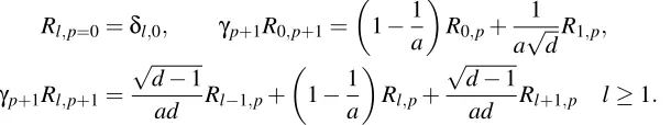
Figure 1 (left) shows the results obtained by iterating Equation (4) numerically for a 3-regular

tree witha=2. As expected the kernel becomes longer-ranged initially aspis increased, but seems

to approach a non-trivial limiting form. This can be calculated analytically and is given by (see Appendix A)

Cl,p_→∞=

1+l(d−2)

d

1

(d₋1)l/2. (5)

Equation (5) can be derived by taking theσ2_{→∞limit of the integral expression for the diffusion}

kernel from Chung and Yau (1999) whilst preserving normalisation of the kernel (see Appendix A.1 for further details). Alternatively the result (5) can be obtained by rewriting the random walk

in terms of shells, that is, grouping vertices according to distance lfrom a chosen central vertex.

The number of vertices in thel-th shell, or shell volume, isvl =d(d₋1)l−1_{forl≥1 andv0=1.}

IntroducingRl,p=Cl,p√vl, Equation (4) can be written in the form

Rl,p=0=δl,0, γp+1R0,p+1=

1₋1

a

R0,p+

1

a√dR1,p,

γp+1Rl,p+1=

√

d₋1

ad Rl−1,p+

1₋1

a

Rl,p+

√

d₋1

ad Rl+1,p l≥1.

(6)

This is just the un-normalised diffusion equation for a biased random walk on a one dimensional lattice with a reflective boundary at 0. This has been solved in Monthus and Texier (1996), and

mapping this solution back toCl,pgives (5) (see Appendix A.2 for further details).

To summarise thus far, the analysis on ad-regular tree shows that, for largep, the random walk

kernel does not approach the expected fully correlated limit: because all vertices have the same

degree this limit would correspond toCl,p→∞=1. On the other hand, on ad-regular graph with any

finite numberV of vertices, the fully correlated limit must necessarily be approached asp_→∞. As

a large regular graph is locally treelike, the difference must arise from the existence of long cycles in a regular graph.

To estimate when the existence of cycles will start to affect the kernel, consider first ad-regular

tree truncated at depthl. This will haveV=1+∑li=1d(d−1)i−1=O(d(d−1)l−1)vertices. On a

d-regular graph with the same number of vertices, we therefore expect to encounter cycles after a

number of steps, taken along the graph, of orderl. In the random walk kernel the typical number of

steps isp/a, so effects of cycles should appear oncep/abecomes larger than

p

a ≈

log(V)

log(d₋1). (7)

Figure 1 (right) shows a comparison betweenC1,pas calculated from Equation (4) for a 3-regular

0 0.2 0.4 0.6 0.8 1

0 2 4 6 8 10 12 14

Cl,

p

l

0.1 0.2 0.3 0.4 0.5 0.6 0.7 0.8 0.9 1

1 10 100 1000

K1

,

p

p/a

log(V)/log(d₋1)

p=1

p=2

p=3

p=4

p=5

p=10

p=20

p=50

p=100

p=200

p=500

p=∞

a=2,V=∞

a=2,V=500

a=4,V=∞

a=4,V=500

Figure 1: (Left) Random walk kernelCl,pon a 3-regular tree plotted against distancelfor increasing

number of steps p and a=2. (Right) Comparison between numerical results for the

average nearest neighbour kernelK1,pon random 3-regular graphs with the resultC1,pon

a 3-regular tree, calculated numerically by iteration of (4).

analogue as the average ofCi j/p

CiiCj j over all pairs of neighbouring vertices on a fixed graph,

averaged further over a number of randomly generated regular graphs. The square root accounts

for the fact that local kernel valuesCiican vary slightly on a regular graph because of cycles, while

they are the same for all vertices of a regular tree. Looking at Figure 1 (right) one sees that, as expected from the arguments above, the nearest neighbour kernel value for the 3-regular graph,

K1,p, coincides with its analogueC1,p on the 3-regular tree for small p. When p/a crosses the

threshold (7), cycles in the regular graph become important and the two curves separate. For larger

p, the kernel value for neighbouring vertices approaches the fully correlated limit K1,p →1 on a

regular graph, while on a regular tree one has the non-trivial limitC1,p→2

√

d−1/dfrom (5).

In conclusion of our analysis of random walk kernels, we have seen that these kernels have

an unusual dependence on their lengthscale p/a. In particular, kernel values for vertices a short

distance apart can remain significantly below the fully correlated limit, even if p/ais large. That

limit is approached only once p/abecomes larger than the graph size-dependent threshold (7), at

which point cycles become important. We have focused here on random regular graphs, but the same qualitative behaviour should be observed also on graphs with a non-trivial distribution of

vertex degreesdi.

3. Learning Curves for Gaussian Process Regression

regres-sion. For a more comprehensive discussion of GPs for machine learning we direct the reader to Rasmussen and Williams (2005).

3.1 Gaussian Process Regression: Kernels as Covariance Functions

Gaussian process regression is a Bayesian inference technique that constructs a posterior distribution

over a function space,P(f_|x,y), given training input locationsx= (x1, . . . ,xN)Tand corresponding

function value outputsy= (y1, . . . ,yN)T. The posterior is constructed from a prior distributionP(f)

over the function space and the likelihoodP(y_|f,x) to generate the observed output values from

function f by using Bayes’ theorem

P(f_|x,y) =R P(y|f,x)P(f)

df′_P(y|f′_,x)P(f′₎.

In the GP setting the prior is chosen to be a Gaussian process, where any finite number of function

values has a joint Gaussian distribution, with a covariance matrix with entries given by acovariance

functionor kernelC(x,x′)and with a mean vector with entries given by amean function µ(x). For

simplicity we will focus on zero mean GPs1and a Gaussian likelihood, which amounts to assuming

that training outputs are corrupted by independent and identically distributed Gaussian noise. Under these assumptions all distributions are Gaussian and can be calculated explicitly. If we assume we

are given training data_{(xµ,yµ)|µ=1, . . . ,N}whereyµis the value of the target or ‘teacher’ function

at input locationxµ, corrupted by additive Gaussian noise with varianceσ2_{, the posterior distribution}

is then given by another Gaussian process with mean and covariance functions

¯

f(x) =k(x)TK−1y, (8)

Cov(x,x′) =C(x,x′)₋k(x)T_K−1_k(x′_{), (9)}

wherek(x) = (C(x1,x), . . . ,C(xN,x))TandKµν=C(xµ,xν) +δµνσ2. With the posterior in the form

of a Gaussian process, predictions are simple. Assuming a squared loss function, the optimal

pre-diction of the outputs is given by ¯f(x)and a measure of uncertainty in the prediction is provided by

Cov(x,x)1/2_.

Equations (8) and (9) illustrate that, in the setting of GP regression, kernels are used to change the type of function preferred by the Gaussian process prior, and correspondingly the posterior. The kernel can encode prior beliefs about smoothness properties, lengthscale and expected amplitude of

the function we are trying to predict. Of particular importance for the discussion below,C(x,x)gives

the prior variance of the function f at inputx, so thatC(x,x)1/2_{sets the typical functionamplitude}

orscale.

3.2 Kernel Normalisation

Conventionally one fixes the desired scale of the kernel using a global normalisation: denoting

the unnormalised kernel by ˆC(x,x′) one scalesC(x,x′) =_C(xˆ _,x′_{)/κto achieve a desired average}

ofC(x,x)across input locationsx. In Euclidean spaces one typically uses translationally invariant

kernels like the squared exponential kernel. For these,C(x,x)is the same for all input locationsx

and so global normalisation is sufficient to fix a spatially uniform scale for the prior amplitude. In the case of kernels on graphs, on the other hand, the local connectivity structure around each vertex

can be different. Since information about correlations ‘propagates’ only along graph edges, graph kernels are not generally translation invariant. In particular, there can be large variation among the prior variances at different vertices. This is usually undesirable in a probabilistic model, unless one has strong prior knowledge to justify such variation. For the random walk kernel, the local prior variances are the diagonal entries of Equation (3). These are directly related to the probability of return of a lazy random walk on a graph, which depends sensitively on the local graph structure. This dependence is in general non-trivial, and not just expressible through, for example, the degree of the local vertex. It seems difficult to imagine a scenario where such a link between prior variances and local graph structures could be justified by prior knowledge.

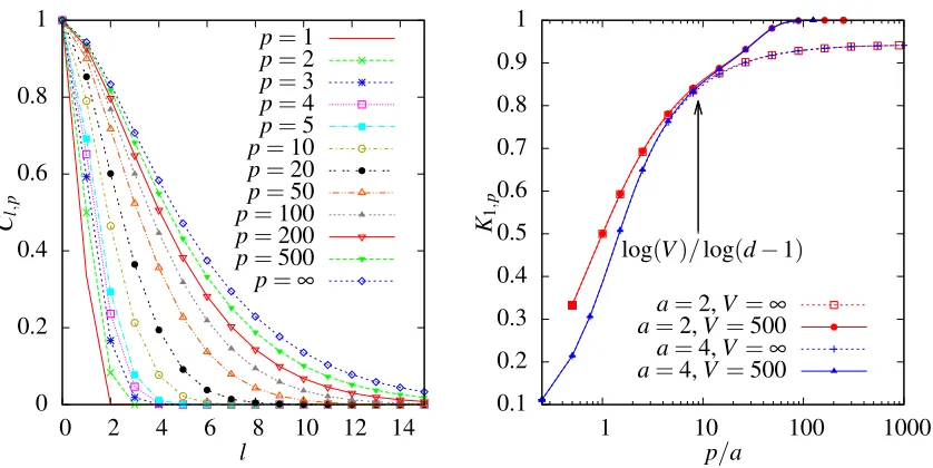
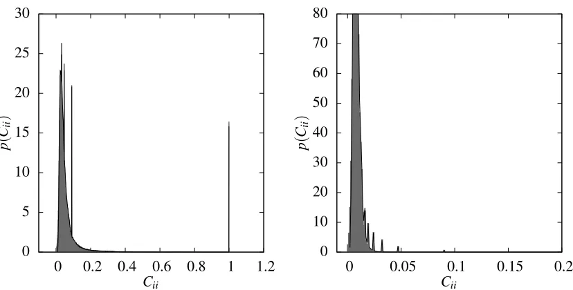
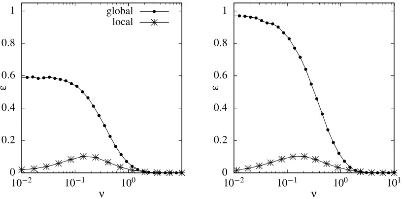
To emphasise the issue, Figure 2 shows examples of distributions of local prior variancesCii

for random walk kernels globally normalised to an average prior variance of unity.2 The

distribu-tions are peaked around the desired value of unity but contain many ‘outliers’ from vertices with

abnormally low or high prior variance. Figure 2 (left) shows the distribution ofCii for a large

single instance of an Erd˝os-R´enyi random graph (Erd˝os and R´enyi, 1959). In such graphs, each edge is present independently of all others with some fixed probability, giving a Poisson

distribu-tion of degrees p_λ(d) =λd_{exp(−λ)/d!; for the figure we chose average degree λ=3. Figure 2}

(right) shows analogous results for a generalised random graph with power law mixing distribution (Britton et al., 2006). Generalised random graphs are an extension of Erd˝os-R´enyi random graphs where different edges are assigned different probabilities of being present. By appropriate choice of these probabilities (Britton et al., 2006), one can generate a degree distribution that is a

superpo-sition of Poisson distributions,p(d) =Rdλpλ(d)p(λ). We have taken a shifted Pareto distribution,

p(λ) =αλα

m/λα+1with exponentα=2.5 and lower cutoffλm=2 for the distribution of the means.

Looking first at Figure 2 (left), we know that large Erd˝os-R´enyi graphs are locally tree-like and hence one might expect that this would lead to relatively uniform local prior variances. As shown in the figure, however, even for such tree-like graphs large variations can exist in the lo-cal prior variances. To give some specific examples, the large spike near 0 is caused by single disconnected vertices and the smaller spike at around 6.8 arises from two-vertex (single edge) dis-connected subgraphs. Single vertex subgraphs have an atypically small prior variance since, for a

single disconnected vertexi, before normalisationCii= (1₋a−1)p_{which is theq=0 contribution}

from Equation (3). Other vertices in the graph will get additional contributions fromq_≥1 and so

have a larger prior variance. This effect will become more pronounced as p is increased and the

binomial weights assign less weight to theq=0 term.

Somewhat surprisingly at first sight, the opposite effect is seen for two-vertex disconnected

subgraphs as shown by the spike aroundCii=6.8 in Figure 2 (left). For vertices on such subgraphs,

Cii=∑⌊_qp₌/₀2⌋ _2qpa−2q(1₋a−1)p−2q_{, which is an atypically large return probability: after any even}

number of steps, the walker must always return to its starting vertex. A similar situation would occur on vertices at the centre of a star. This illustrates that local properties of a vertex alone, like its degree, do not constrain the prior variance. In a two-vertex disconnected subgraph both vertices have degree 1. But there will generically be other vertices of degree 1 that are dangling ends of a large connected graph component, and these will not have similarly elevated return probabilities. Thus, local graph structure is intertwined in a complex manner with local prior variance.

The black line in Figure 2 (left) shows theoretical predictions (see Section 4.2) for the prior variance distribution in the large graph limit. There is significant fine structure in the various peaks,

2. We useCiiagain here, instead ofC(i,i)as in our general discussion of GPs; the subscript notation is more intuitive

on which theory and simulations agree well where the latter give reliable statistics. The decay from the mean is roughly exponential (see linear-log plot in inset), emphasizing that the distribution of local prior variances is not only rather broad but can also have large tails.

For the power law random graph, Figure 2 (right), the broad features of the distribution of local

prior variancesCiiare similar: a peak at the desired value of unity, overlaid by spikes which again

come from single and two-vertex disconnected subgraphs. The inset shows that the tail beyond the mean is roughly exponential again, but with a slower decay; this is to be expected since power law graphs exhibit many more different local structures with a significantly larger probability than is

the case for Erd˝os-R´enyi graphs. Accordingly, the distribution of theCiialso has a larger standard

deviation than for the Erd˝os-R´enyi case. The maximum values ofCiithat we see in these two specific

graph instances follow the same trend, with maxiCii≈40 for the power law graph and maxiCii≈15

for the Erd˝os-R´enyi graph. Such large values would constitute rather unrealistic prior assumptions about the scaling of the target function at these vertices.

To summarise, Figure 2 shows that after global normalisation a random walk kernel can retain a large spread in the local prior variances, with the latter depending on the graph structure in a

compli-cated manner. We propose that to overcome this one should use alocal normalisation. For a desired

prior variancecthis means normalising according toCi j=cCˆi j/(κiκj)1/2with local normalisation

constantsκi =Ciiˆ ; here ˆCi j is the unnormalised kernel matrix as before. This guarantees that all

vertices have exactly equal prior variance as in the Euclidean case, that is, all vertices have a prior

variance ofc. No uncontrolled local variation in the scaling of the function prior then remains, and

the computational overhead of local over global normalisation is negligible. Graphically, if we were to normalise the kernel to unity according to the local prescription, a plot of prior variances like the one in Figure 2 would be a delta peak centred at 1.

The effect of this normalisation on the behaviour of GP regression is a key question for the remainder of this paper; numerical simulation results are shown in Section 3.3 below, while our theoretical analysis is described in Section 4.

3.3 Predicting the Learning Curve

The performance of non-parametric methods such as GPs can be characterised by studying the

learning curve,

ε(N) =

****

1

V V

∑

i=1

gi_{− h}fi_if|x,y

2 +

y_|g,x

+

g

+

x

+

G ,

defined as the average squared error between the student and teacher’s predictionsf= (f1, . . . ,fV)T

andg= (g1, . . . ,gV)T_{respectively, averaged over the student’s posterior distribution given the data}

f_|x,y, the outputs given the teacher y_|g,x, the teacher functions g, and the input locations x.

This gives the average generalisation error as a function of the number of training examples. For simplicity we will assume that the input distribution is uniform across the vertices of the graph.

Because we are analysing GP regression on graphs, after the averages discussed so far the gen-eralisation error will still depend on the structure of the specific graph considered. We therefore

include an additional average, over all graphs in a random graph ensemble

G

ensembles defined by the distribution of degreesdi: we specify a degree sequence{d1, . . . ,dV}, or,

for largeV, equivalently a degree distribution p(d), and pick uniformly at random any one of the

0 0.5 1 1.5 2 2.5 3 3.5

0 1 2 3 4 5 6 7 8 9

p

(

Cii

)

Cii

0 0.5 1 1.5 2 2.5 3 3.5

0 1 2 3 4 5 6 7 8 9

p

(

Cii

)

Cii

10−4

10−3

10−2

10−1

100

2 3 4

10−4

10−3

10−2

10−1

100

1 2 3 4

Figure 2: (Left) Grey: histogram of prior variances for the globally normalised random walk kernel

witha=2,p=10 on a single instance of an Erd˝os-R´enyi graph with mean degreeλ=3

andV =10000 vertices. Black: prediction for this distribution in the large graph limit

(see Section 4.2). Inset: Linear-log plot of the tail of the distribution. (Right) As (left) but for a power law generalised random graph with exponent 2.5 and cutoff 2.

as long as it has finite mean. Our analysis therefore has broad applicability, including in

particu-lar the graph types already mentioned above (d-regular graphs, where p(d′) =δdd′, Erd˝os-R´enyi

graphs, power law generalised random graphs).

For this paper, as is typical for learning curve studies, we will assume that teacher and stu-dent have the same prior distribution over functions, and likewise that the assumed Gaussian noise

of varianceσ2 _{reflects the actual noise process corrupting the training data. This is known as the}

matched case.3 Under this assumption the generalisation error becomes the Bayes error, which given that we are considering squared error simplifies to the posterior variance of the student aver-aged over data sets and graphs (Rasmussen and Williams, 2005). Since we only need the posterior

variance we shiftf so that the posterior mean is0_{; fiis then just the deviation of the function value}

at vertexifrom the posterior mean. The Bayes error can now be written as

ε(N) =

***

1

V V

∑

i=1 f_i2

+

f_|x

+

x

+

G

. (10)

Note that by shifting the posterior distribution to zero mean, we have eliminated the dependence

on y in the above equation. That this should be so can also be seen from (9) for the posterior

(co-)variance, which only depends on training inputsxbut not the corresponding outputsy.

The averages in Equation (10) are in general difficult to calculate analytically, because the

train-ing input locations xenter in a highly nonlinear matter, see (9); only for very specific situations

can exact results be obtained (Malzahn and Opper, 2005; Rasmussen and Williams, 2005). Approx-imate learning curve predictions have been derived, for Euclidean input spaces, with some degree of success (Sollich, 1999a,b; Opper and Vivarelli, 1999; Williams and Vivarelli, 2000; Malzahn and Opper, 2003; Sollich, 2002; Sollich and Halees, 2002; Sollich and Williams, 2005). We will show that in the case of GP regression for functions defined on graphs, learning curves can be predicted exactly in the limit of large random graphs. This prediction is broadly applicable because the degree distribution that specifies the graph ensemble is essentially arbitrary.

It is instructive to begin our analysis by extending a previous approximation seen in Sollich (1999a) and Malzahn and Opper (2005) to our discrete graph case. In so doing we will see explicitly how one may improve this approximation to fully exploit the structure of random graphs, using

belief propagation or equivalently thecavity method(M´ezard and Parisi, 2003). We will sketch the

derivation of the existing approximation following the method of Malzahn and Opper (2005); the result given by Sollich (1999a) is included in this as a somewhat more restricted approximation. Both the approximate treatment and our cavity method take a statistical mechanics approach, so we

begin by rewriting Equation (10) in terms of ageneratingorpartition function Z

ε(N) =

*

1

V

∑

dfP(f_|x)f_i2

+

x,G

=₋lim

λ→0

2

V

∂

∂λhlog(Z)ix,G, (11)

with

Z=

Z

dfexp ₋1

2f

T_C−1_f

−_2σ12 N

∑

µ=1 f_x2_µ−λ

2

∑

2 i

!

.

In this representation the inputsxonly enterZthrough the sum overµ. We introduceγito count the

number of examples at vertexiso thatZbecomes

Z=

Z

dfexp

−1₂fTC−1f₋1

2f

T_diagγi

σ2+λ

f

. (12)

The average in Equation (11) of the logarithm of this partition function can still not be carried out in closed form. The approximation given by Malzahn and Opper (2005) and our present cavity approach diverge at this point. Section 3.4 discusses the existing approximation for the learning curve, applied to the case of regression on a graph. Section 4 then improves on this using the cavity method to fully exploit the graph structure.

3.4 Kernel Eigenvalue Approximation

The approach of Malzahn and Opper (2005) is to average log(Z)from (12) using the replica trick

(M´ezard et al., 1987). One writes _hlogZ_ix =limn_→0_n1loghZnix, performing the average hZnix

for integern and assuming that a continuation ton_→0 is possible. The requiredn-th power of

Equation (12) is given by

hZn_ix= Z n

∏

a=1

dfa

*

exp ₋1

2

∑

a₎T_C−1_fa₋ 1

2σ2

∑

i,a

γi(fia)2−

λ

2

∑

a i )2

!+

where the replica indexaruns from 1 ton. Assuming as before that examples are generated

inde-pendently and uniformly from

V

to independent Poisson averages overγi with meanν=N/V. Explicitly performing these averages

gives

hZn_ix= Z n

∏

a=1

dfaexp ₋1

2

∑

a₎T_C−1_fa_+ν

_∑

e−∑a(fia)2/2σ2−₁

−λ

2

∑

a i )2

!

. (13)

In order to evaluate (13) one has to find a way to deal with the exponential term in the exponent.

Malzahn and Opper (2005) do this using a variational approximation for the distribution of thefa,

of Gaussian form. Eventually this leads to the following eigenvalue learning curve approximation (see also Sollich, 1999a):

ε(N) =g

N

ε(N) +σ2

, g(h) =

V

∑

α=1

λ−_α1+h−1. (14)

The eigenvaluesλαof the kernel are defined here from the eigenvalue equation4 (1/V)∑jCi jφj=

λφi. The Gaussian variational approach is evidently justified for largeσ2, where a Taylor expansion

of the exponential term in (13) can be truncated after the quadratic term. For small noise levels, on the other hand, the Gaussian variational approach will in general not capture all the details of the

fluctuations in the numbers of examplesγi. This issue is expected to be most prominent for values

ofνof order unity, where fluctuations in the number of examples are most relevant because some

vertices will not have seen examples locally or nearby and will have posterior variance close to the

prior variance, whereas those vertices with examples will have small posterior variance, of orderσ2_.

This effect disappears again for largeν, where theO(√ν)fluctuations in the number of examples at

each vertex becomes relatively small. Mathematically this can be seen from the term proportional

toνin (13), which for largeνensures that only values of f_iawith exp(₋∑a(fia)2/2σ2)close to 1

will contribute. A quadratic approximation is then justified even ifσ2_{is not large.}

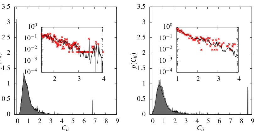
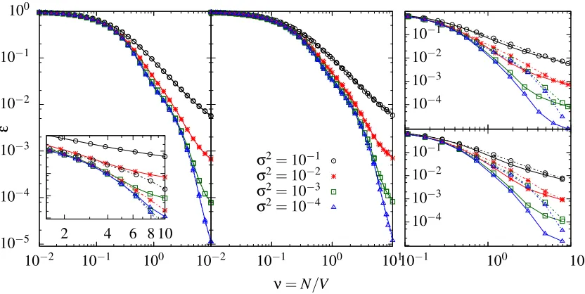
Learning curve predictions from Equation (14) using numerically computed eigenvalues for the globally normalised random walk kernel are shown in Figure 3 as dotted lines for random regular (left), Erd˝os-R´enyi (centre) and power law generalised random graphs (right). The predictions are compared to numerically simulated learning curves shown as solid lines, for a range of noise levels. Consistent with the discussion above, the predictions of the eigenvalue approximation are accurate

where the Gaussian variational approach is justified, that is, for small and largeν. Figure 3 also

shows that the accuracy of the approximation improves as the noise levelσ2_{becomes larger, again}

as expected by the nature of the Gaussian approximation.

3.4.1 LEARNINGCURVES FORLARGE p

Before moving on to the more accurate cavity prediction of the learning curves, we now look at

how the learning curves for GP regression on graphs depend on the kernel lengthscale p/a. We

focus for this discussion on random regular graphs, where the distinction between global and local normalisation is not important. In Section 2.1, we saw that on a large regular graph the random walk

kernel approaches a non-trivial limiting form for large p, as long as one stays below the threshold

10−5

10−4

10−3

10−2

10−1

100

10−2 10−1 100

ε

10−2 10−1 100

ν=N/V

10−2 10−1 100 101

σ2₌₁₀−1

σ2₌₁₀−2

σ2₌₁₀−3

σ2₌₁₀−4

Figure 3: (Left) Learning curves for GP regression with globally normalised kernels with p=10,

a=2 on 3-regular random graphs for a range of noise levels σ2_{. Dotted lines:}

eigen-value predictions (see Section 3.4), solid lines: numerically simulated learning curves

for graphs of sizeV =500, dashed lines: cavity predictions (see Section 4.1); note these

are mostly visually indistinguishable from the simulation results. (Centre) As (left) for Erd˝os-R´enyi random graphs with mean degree 3. (Right) As (left) for power law gener-alised random graphs with exponent 2.5 and cutoff 2.

(7) for p where cycles become important. One might be tempted to conclude from this that also

the learning curves have a limiting form for large p. This is too naive however, as one can see by

considering, for example, the effect of the first example on the Bayes error. If the example is at

vertexi, the posterior variance at vertex jis, from (9),Cj j−Ci j2/(Cii+σ2). As the prior variances

Cj j are all equal, to unity for our chosen normalisation, this is 1−C2i j/(1+σ2). The reduction in

the Bayes error is thereforeε(0)₋ε(1) = (1/V)∑jC2i j/(1+σ2). As long as cycles are unimportant

this is independent of the location of the example vertexi, and in the notation of Section 2.1 can be

written as

ε(0)₋ε(1) = 1

1+σ2

p

∑

l=0

vlC_l2_,p, (15)

where vl is, as before, the number of vertices a distance l away from vertex i, that is, v0 =1,

vl =d(d−1)l−1 for l≥1. To evaluate (15) for large p, one cannot directly plug in the limiting

kernel form (5): the ‘shell volume’vljust balances thel-dependence of the factor(d₋1)−l/2_from

Cl,p, so that one gets contributions from all distances l, proportional to l2 for large l. Naively

summing up tol=pwould give an initial decrease of the Bayes error growing as p3. This is not

correct; the reason is that whileCl,papproaches the large p-limit (5) for any fixedl, it does so more

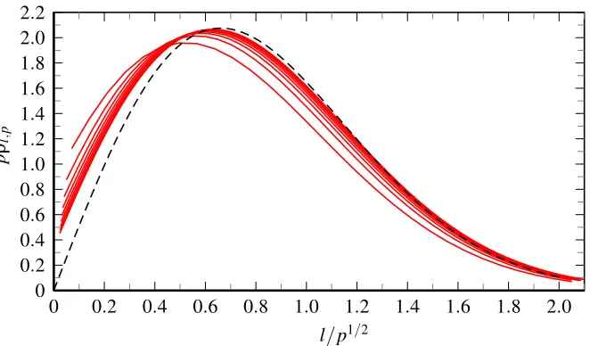
for large land p,Cl,p is proportional to the large p-limit l(d−1)−l/2 up to a characteristic cutoff

distancelof orderp1/2, and decays quickly beyond this. Summing in (15) the contributions of order

l2up to this distance predicts finally that the initial error decay should scale, non-trivially, as p3/2.

We next show that this large p-scaling with p3/2is also predicted, for the entire learning curve,

by the eigenvalue approximation (14). As before we considerd-regular random graphs. The

re-quired spectrum of kernel eigenvaluesλαbecomes identical, for largeV, to that on ad-regular tree

(McKay, 1981). Explicitly, ifλL

αare the eigenvalues of the normalised graph Laplacian on a tree,

then the kernel eigenvalues are λα=κ−1V−1(1−λLα/a)p. Here the factorV−1 comes from the

same factor in the kernel eigenvalue definition after (14), andκis the overall normalisation constant

which enforces∑αλα=V−1∑jCj j=1. The spectrum of the tree Laplacian is known (see McKay,

1981; Chung, 1996) and is given by

ρ(λL_{) =}







q

4(d−1)

d2 −(λL−1)2

(2π/d)λL_(2−λL₎ λ−≤λ≤λ+,

0 otherwise,

where λ_±=1_±2_d(d₋1)1/2_{. (There are also two isolated eigenvalues at 0 and 2, which do not}

contribute for largeV.)

We can now write down the functiongfrom (14), converting the sum over kernel eigenvalues to

V times an integral over Laplacian eigenvalues for largeV. Dropping theLsuperscript, the result is

g(h) = Z λ+

λ−

dλ ρ(λ)[κ(1−λ/a)−p_+hV−1_]−1_{. (16)}

The dependence onhV−1 here shows that in the approximate learning curve (14), the Bayes error

will depend only onν=N/V as might have been expected. The condition for the normalisation

factorκbecomes simplyg(0) =1, orκ−1₌R_{dλ ρ(λ)(1−λ/a)}p_.

So far we have written down how one would evaluate the eigenvalue approximation to the

learn-ing curve on larged-regular random graphs, for arbitrary kernel parameters panda. Now we want

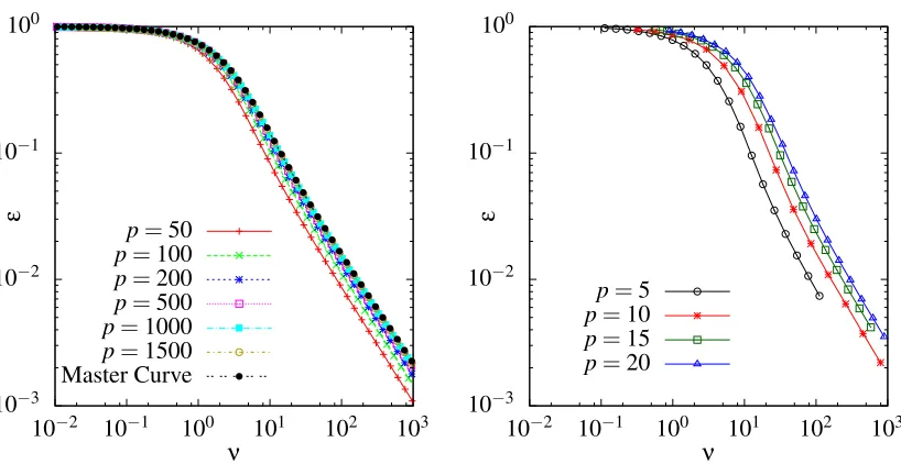
to consider the largep-limit. We show that there is then amaster curvefor the Bayes error against

νp3/2_{. This is entirely consistent with thep}3/2_{scaling found above for the initial error decay. The}

intuition for the largepanalysis is that the factor(1₋λ/a)p_{decays quickly as the Laplacian}

eigen-valueλincreases beyondλ₋, so that only values ofλnearλ₋contribute. One can then approximate

1₋λ

a

p ≈

1₋λ−

a

p

exp

−p(λ−λ−)

a₋λ₋

.

Similarly one can replaceρ(λ)by its leading square root behaviour nearλ₋,

ρ(λ) = (λ₋λ₋)1/2(d−1) 1/4_d5/2

π(d₋2)2 .

Substituting these approximations into (16) and introducing the rescaled integration variable y=

p(λ₋λ₋)/(a₋λ₋)gives

g(h) =rκ−1(1₋λ₋/a)p

a₋λ₋

p

3/2

10−3

10−2

10−1

100

10−2 10−1 100 101 102 103

ε

ν

10−3

10−2

10−1

100

10−2 10−1 100 101 102 103

ε

ν

p=50

p=100

p=200

p=500

p=1000

p=1500 Master Curve

p=5

p=10

p=15

p=20

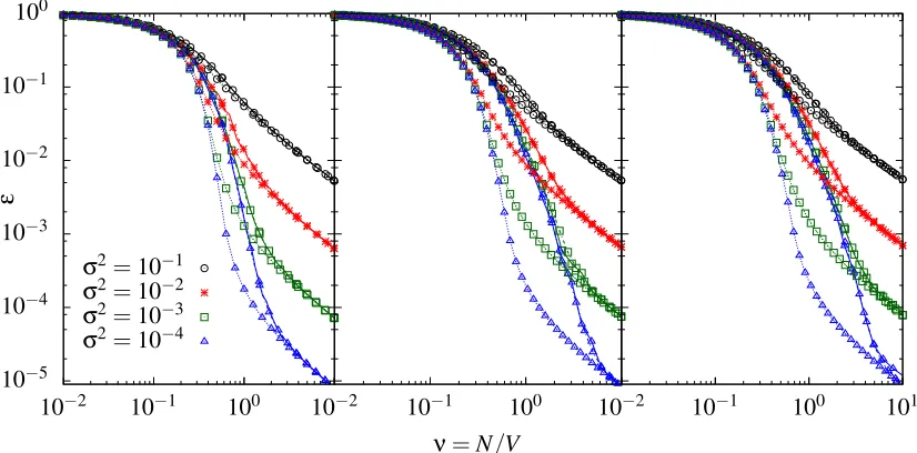
Figure 4: (Left) Eigenvalue approximation for learning curves on a random 3-regular graph, using

a random walk kernel witha=2,σ2_{=0.1 and increasing values ofpas shown. Plotting}

against νp3/2 shows that for large p these rescaled curves approach the master curve

predicted from (17), though this approach is slower in the tail of the curves. (Right) As

(left), but for numerically simulated learning curves on graphs of sizeV =500.

where r= (d₋1)1/4_d5/2_/(π(d−2)2_{) andF(z) =}R∞

0 dy y1/2(exp(y) +z)−1. Since g(0) =1, the

prefactor must equal 1/F(0) =2/√π. This fixes the normalisation constantκ, and we can simplify

to

g(h) =F(hV− 1_c−1₎

F(0) , c=rF(0)

a₋λ₋

p

3/2

.

The learning curves for large pare then predicted from (14) by solving

ε=F(νc−1/(ε+σ2))/F(0), (17)

and depend clearly only on the combinationνc−1. Because cis proportional to p−3/2, this shows

that learning curves for differentpshould collapse onto a master curve when plotted againstνp3/2.

A plot of the scaling of the eigenvalue learning curve approximations onto the master curve

is shown in Figure 4 (left). As can be seen, large values of p are required in order to get a good

collapse in the tail of the learning curve prediction, whereas in the initial part the p3/2 scaling is

accurate already for relatively smallp.

Finally, Figure 4 (right) shows that the predicted p3/2-scaling of the learning curves is present

not only within the eigenvalue approximation, but also in the actual learning curves. Figure 4

(right) displays numerically simulated learning curves forp=5,10,15 and 20, against the rescaled

number of examplesνp3/2as before. Even for these comparatively small values of pone sees that

4. Exact Learning Curves: Cavity Method

So far we have discussed the eigenvalue approximation of GP learning curves, and how it deviates from numerically exact simulated learning curves. As discussed in Section 3.4, the deficiencies of the eigenvalue approximation can be traced back to the fact that the fluctuations in the number of training examples seen at each vertex of the graph cannot be accounted for in detail. If in the average over data sets these fluctuations could be treated exactly, one would hope to obtain exact, or at least very accurate, learning curve predictions. In this section we show that this is indeed possible in the case of a random walk kernel, for both global and local normalisations. We derive our prediction using belief propagation or, equivalently, the cavity method (M´ezard and Parisi, 2003). The approach relies on the fact that the local structure of the graph on which we are learning is tree-like. This local tree-like structure always occurs in large random graphs sampled uniformly from an ensemble specified by an arbitrary but fixed degree distribution, which is the scenario we

consider here. We will see that already for moderate graph sizes ofV =500, our predictions are

nearly indistinguishable from numerical simulations.

In order to apply the cavity method to the problem of predicting learning curves we must first rewrite the partition function (12) in the form of a graphical model. This means that the function

being integrated over to obtainZ must consist of factors relating only to individual vertices, or to

pairs of neighbouring vertices. The inverse of the covariance matrix in (12) creates factors linking vertices at arbitrary distances along the graph, and so must be eliminated before the cavity method

can be applied. We begin by assuming a general form for the normalisation of ˆCthat encompasses

both local and global normalisation and setC =

K

_K

with

Ki j

term exp(₋1₂fT_C−1_{f)in (12), introduce Fourier variablesh, and then integrate out the remaining}

terms with respect tof to give

Z∝

_∏

i

γ_i σ2+λ

−1/2Z

dhexp

−1₂hTCh₋1

2h

T_diag

γ_i

σ2+λ

−1/2

h

.

The coupling between different vertices in (4) is now throughCso still links vertices up to distance

p. To reduce these remaining interactions to ones among nearest neighbours only, one exploits

the binomial expansion of the random walk kernel given in (3). Defining padditional variables at

each vertex ashq=

K

_K

q= _qp

(1₋

a−1)p−q_(a−1₎q_{, the interaction termh}T_{Chturns into a local term∑}p

q=0cq(h0)T

K

have, for the sake of uniformity, written h0 instead ofh.) Of course the interactions have only

been ‘hidden’ in thehq_{, but the key point is that the definition of these additional variables can be}

enforced recursively, viahq=

K

K

Dirac delta function (for eachq=1, . . . ,p) and then Fourier transform the latter, with conjugate

variablesˆhq_{, to get}

Z∝

_∏

i

γ_i σ2+λ

−1/2Z p

∏

q=0

dhq

p

∏

q=1

dˆhqexp ₋1

2(h

0₎T_diag

γ_i

σ2+λ

−1

h0

−1₂

p

∑

q=0

cq(h0)T

K

∑

q=1

(ˆ_hq₎T_hq

−

K

K

!

Because the graph adjacency matrixAnow appears at most linearly in the exponent, all interactions

are between nearest neighbours only. We have thus expressed ourZas the partition function of a

(complex-valued) graphical model.

4.1 Global Normalisation

We can now apply belief propagation to the calculation of marginals for the above graphical model.

We focus first on the simpler case of a globally normalised kernel whereκi=κfor alli. Rescaling

eachhq_i tod_i1/2κ1/2_hq

i and ˆh

q i tod

1/2 i hˆ

q

i/κ1/2we are left with

Z∝

_∏

i

γ_i σ2+λ

−1/2Z p

∏

q=0

dhq

p

∏

q=1

dˆhq

∏

i

exp ₋1

2

p

∑

q=0 cqh0ih

q idi−

1 2

(h0 i)2κdi

γi/σ2+λ +i

p

∑

q=1 dihˆqih

q i

!

∏

(i,j)

exp ₋i

p

∑

q=1

ˆ

hq_ihq_j−1+_hˆq jh

q₋1 i

!

, (19)

where the interaction terms coming from the adjacency matrix,A, have been written explicitly as a

product over distinct graph edges(i,j).

To see how the Bayes error (10) can be obtained from this partition function, we differentiate

log(Z)with respect toλas prescribed by (11) to get

ε(ν) =lim

λ→0

1

V

∑

1

γi/σ2+λ

1₋diκh(h

0 i)2i

γi/σ2+λ

. (20)

In order to calculate the Bayes error we therefore require specifically the marginal distributions of

h0_i. These can be calculated using the cavity method: for a large random graph with arbitrary fixed

degree sequence the graph is locally tree-like, so that if vertexiwere eliminated the corresponding

subgraphs (locally trees) rooted at the neighbours j_∈

N

in-dependent. The resulting cavity marginals created by removingi, which we denoteP(_ji)(hj,ˆhj|x),

can then be calculated iteratively within these subgraphs using the update equations

P(_ji)(hj,ˆhj|x)∝exp −

1 2

p

∑

q=0

cqdjh0jh q j−

1 2

djκ(h0j)2

γj/σ2+λ +i

p

∑

q=1 djhˆqjh

q j

!

Z

∏

k∈N(j)\i

dhkdˆhkexp −i

p

∑

q=1

(hˆq_jhq_k−1+hˆq_khq_j−1)

!

P_k(j)(hk,hˆk|x). (21)

wherehj= (h0j, . . . ,h

p

j)Tandˆhj= (hˆ1j, . . . ,hˆ p

j)T. In terms of the sum-product formulation of belief

propagation, the cavity marginal on the left is the message that vertex jsends to the factor inZfor

edge(i,j)(Bishop, 2007).

One sees that the cavity update Equations (21) are solved self-consistently by complex-valued

Gaussian distributions with mean zero and covariance matricesV_j(i). This Gaussian character of

the solution was of course to be expected because in (19) we have a Gaussian graphical model. By performing the Gaussian integrals in the cavity update equations explicitly, one finds for the corresponding updates of the covariance matrices the rather simple form

V_j(i)= (Oj−

∑

where we have defined the(2p+1)_×(2p+1)matrices

Oj=dj

            

c0+_γ κ

j/σ2+λ

c1 2 . . .

cp

2 0 . . . 0 c1

2 −i

..

. . ..

cp

2 −i

0 ₋i

..

. . .. 0_p,p

0 ₋i

            

, X=

            i

0_p+1,p+1 . ..

i 0 . . . 0

i 0

. .. .._{. 0}

p,p

i 0             . (23)

At first glance (22) becomes singular forγj=0; however this is easily avoided. We introduce

Oj−∑d_k=−11XV

(j)

k X =Mj+ [djκ/(γj/σ

2_+λ)]e

0eT0 witheT0 = (1,0, . . . ,0) so thatMj contains

all the non-singular terms. We may then apply the Woodbury identity (Hager, 1989) to write the

matrix inverse in a form where theλ_→0 limit can be taken without difficulties:

Oj− d−1

∑

k=1

XV_k(j)X

!−1

=M−_j 1₋ M −1

j e0eT0Mj−1 (γj/σ2+λ)/(djκ) +eT0M−

1 j e0

.

In our derivation so far we have assumed a fixed graph, we therefore need to translate these equations to the setting we ultimately want to study, that is, an ensemble of large random graphs.

This ensemble is characterised by the distributionp(d)of the degreesdi, so that every graph that has

the desired degree distribution is assigned equal probability. Instead of individual cavity covariance

matrices V_j(i), one must then consider their probability distributionW(V)across all edges of the

graph. Picking at random an edge(i,j)of a graph, the probability that vertex jwill have degree

dj is then p(dj)dj/d¯, because such a vertex hasdj ‘chances’ of being picked. (The normalisation

factor is the average degree ¯d=∑ip(di)di.) Using again the locally treelike structure, the incoming

(to vertex j) cavity covariancesV_k(j)will be independent and identically distributed samples from

W(V). Thus a fixed point of the cavity update equations corresponds to a fixed point of an update

equation forW(V):

W(V) =

_∑

d p(d)d

¯

d

*Z

d₋1

∏

k=1

dVkW(Vk)δ



V − O−

d−1

∑

k=1

XVkX

!−1 

+

γ

. (24)

Since the vertex label is now arbitrary, we have omitted the index j. The average in (24) is over the

distribution of the number of examplesγ_≡γj at vertex j. As before we assume for simplicity that

examples are drawn with uniform input probability across all vertices, so that the distribution ofγis

simplyγ_∼Poisson(ν)in the limit of largeNandV at fixedν=N/V.

In general Equation (24)—which can also be formally derived using the replica approach (see Urry and Sollich, 2012)—cannot be solved analytically, but we can tackle it numerically using population dynamics (M´ezard and Parisi, 2001). This is an iterative technique where one creates a population of covariance matrices and for each iteration updates a random element of the population according to the delta function in (24). The update is calculated by sampling from the degree

from the distributionW(Vk) of ‘incoming’ covariance matrices, the latter being approximated by

uniform sampling from the current population.

Once we haveW(V), the Bayes error can be found from the graph ensemble version of

Equa-tion (11). This is obtained by inserting the explicit expression for_h(h0

i)2i in terms of the cavity

marginals of the neighbouring vertices, and replacing the average over vertices with an average over

degreesd:

ε(ν) =lim

λ→0

∑

*

1

γ/σ2_+λ 1− dκ γ/σ2_+λ

Z d

∏

k=1

dVkW(Vk) (O− d

∑

k=1

XVkX)−₀₀1

!+

γ

. (25)

The number of examples at the vertex γis once more to be averaged overγ_∼Poisson(ν). The

subscript ‘00’ indicates the top left element of the matrix, which determines the variance ofh0.

To be able to use Equation (25), we again need to rewrite it into a form that remains

ex-plicitly non-singular when γ=0 and λ_→ 0. We separate the γ-dependence of the matrix

in-verse again and write, in slightly modified notation as appropriate for the graph ensemble case,

O₋∑dk=1XVkX =Md+ [dκ/(γ/σ2+λ)]e0eT0, whereeT0 = (1,0, . . . ,0). The 00 element of the

matrix inverse appearing above can then be expressed using the Woodbury formula (Hager, 1989) as

eT₀ O₋ d

∑

k=1

XVkX

!−1

e0=eT₀M_d−1e0₋ e T

0Md−1e0eT0Md−1e0 (γ/σ2_{+λ)/(dκ) +e}T

0M− 1 d e0

.

Theλ_→0 limit can now be taken, with the result

ε(ν) =

*

∑

d p(d)

Z d

∏

k=1

dVkW(Vk)

1

γ/σ2_+dκ(M−1 d )00

+

γ

. (26)

This has a simple interpretation: the cavity marginals of the neighbours provide an effective

Gaus-sian prior for each vertex, whose inverse variance isdκ(M−1₎

00.

The self-consistency Equation (24) forW(V)and the expression (26) for the resulting Bayes

error allow us to predict learning curves as a function of the number of examples per vertex,ν, for

arbitrary degree distributions p(d)of our random graph ensemble. For large graphs the predictions should become exact. It is worth stressing that such exact learning curve predictions have previously only been available in very specific, noise-free, GP regression scenarios, while our result for GP regression on graphs is applicable to a broad range of random graph ensembles, with arbitrary noise levels and kernel parameters.

We note briefly that for graphs with isolated vertices (d =0), one has to be slightly careful:

already in the definition of the covariance function (2) one should replaceD_→D+δI to avoid

division by zero, taking δ_→0 at the end. For d=0 one then finds in the expression (26) that

(M−1_{)00 =1/(c0δ), where c0 is defined before (18). As a consequence, κ(δ+d)(M}−1₎₀₀₌

κδ(M−1₎

00=κ/c0. This is to be expected since isolated vertices each have a separate Gaussian

prior with variancec0/κ.

Equations (24) and (26) still require the normalisation constant,κ. The simplest way to calculate

this is to run the population dynamics once forκ=1 andν=0, that is, an unnormalised kernel and

no training data. The result forεthen just gives the average (over vertices) prior variance. With

κset to this value, one can then run the population dynamics for any νto obtain the Bayes error

Comparisons between the cavity prediction for the learning curves, numerically exact simu-lated learning curves and the results of the eigenvalue approximation are shown in Figure 3 (left, centre and right), for regular, Erd˝os-R´enyi and generalised random graphs with power law degree distributions respectively. As can be seen the cavity predictions greatly outperform the eigenvalue approximation and are accurate along the whole length of the curve. This confirms our expecta-tion that the cavity approach will become exact on large graphs, although it is remarkable that the agreement is quantitatively so good already for graphs with only five hundred vertices.

4.2 Predicting Prior Variances

As a by-product of the cavity analysis for globally normalised kernels we note that in the cavity form

of the Bayes error in Equation (26), the fraction(γ/σ2_+dκ(M−1

d )00)−1is the local Bayes error,

that is, the local posterior variance. By keeping track of individual samples for this quantity from the population dynamics approach, we can thus predict the distribution of local posterior variances.

If we setν=0, then this becomes the distribution of prior variances. The cavity approach therefore

gives us, without additional effort, a prediction for this distribution.

We can now go back to Section 3.2 and compare the cavity predictions to numerically simulated distributions of prior variances. The cavity predictions for these distributions are shown by the black lines in Figure 2. The cavity approach provides, in particular, detailed information about the tail of the distributions as shown in the insets. There is good agreement between the predictions and the numerical simulations, both regarding the general shape of the variance distributions and the fine structure with a number of non-trivial peaks and troughs. The residual small shifts between the predictions and the numerical results for a single instance of a large graph are most likely due to finite size effects: in a finite graph, the assumption of a tree-like local structure is not exact because there can be rare short cycles; also, the long cycles that the cavity method ignores because their

length diverges logarithmically withV will have an effect whenV is finite.

4.3 Local Normalisation

We now extend the cavity analysis for the learning curves to the case of locally normalised random walk kernels, which, as argued above, provide more plausible probabilistic models. In this case the

diagonal entries of the normalisation matrix

K

κi= Z

dff_i2P(f),

where P(f) is the GP prior with the unnormalised kernel Cˆ. This makes clear why the locally

normalised kernel case is more challenging technically: we cannot calculate the normalisation

con-stants once and for all for a given random graph ensemble and set of kernel parameters pandaas

we did forκin the globally normalised scenario. Instead we have to account for the dependence of

theκion the specific graph instance.

On a single graph instance, this stumbling block can be overcome as follows. One iterates the

cavity updates (22) for the unnormalised kernel and without the training data (i.e., settingκ=1 and

γi=0). The local Bayes error at vertexi, given by thei-th term in the sum from (20), then gives us

κi. Becauseγi=0, one has to use the Woodbury trick to get well-behaved expressions in the limit

Once theκihave been determined in this way, one can use them for predicting the Bayes error

for the scenario we really want to study, that is, using a locally normalised kernel and incorporating the training data. The relevant partition function is the analogue of (18) for local normalisation.

Dropping the prefactors, the resultingZcan be written as

Z∝

Z p

∏

q=0

dhq

p

∏

q=1

dˆhq

∏

i

exp ₋1

2

p

∑

q=0

cqdih0_ihq_{i −}1

2

diκi(h0 i)2

γi/σ2+λ +i

p

∑

q=1 dihˆq_ihq_i

!

∏

(i,j)

exp ₋i

p

∑

q=1

(hˆq_ihq_j−1+hˆq_jhq_i−1)

!

,

where we have rescaledhq_i tod1_i/2κ1_i/2hq_i and ˆh_iqtod_i1/2κ_i−1/2hˆq_i. Given that theκihave already been

determined, this is a graphical model for which marginals can be calculated by iterating to a fixed point the equations for the cavity marginals:

P_loc(i)_,j(hj,ˆhj|x)∝exp −

1 2

p

∑

q=0

cqdjh0jh q

j−

1 2

djκj(h0j)2

γj/σ2+λ +i

p

∑

q=1 djhˆqjh

q j

!

Z

∏

k∈N(j)\i

dhkdˆhkexp −i

p

∑

q=1

(hˆq_jhq_k−1+hˆq_khq_j−1)

!

P_loc(j)_,k(hk,hˆk|x). (27)

As in Section 4.1 these update equations are solved by cavity marginals of complex Gaussian form, and so we can simplify them to updates for the covariance matrices:

V_loc(i)_,j= Oloc,j−

∑

XV_k(_,locj)X

!−1

. (28)

Here X is defined as in Equation (23) and Oloc,j is the obvious analogue of Oj also defined in

Equation (23); specifically,κis replaced byκj. Once the update equations have converged, one can

calculate the Bayes error from a similarly adapted version of (20).

The above procedure for a single fixed graph now has to be extended to the case of an ensemble

of large random graphs characterised by some degree distribution p(d). The outcome of the first

round of cavity updates, for the unnormalised kernel without training data, is then represented by a

distribution of cavity covariancesV, while the second one gives a distribution of cavity covariances

Vloc for the locally normalised kernel, with training data included. Importantly, these message

distributions are coupled to each other via the graph structure, so we need to look at the joint

distributionW(Vloc,V).

Detailed analysis using the replica method (Urry and Sollich, 2012) shows that the correct fixed

point equation updates theV-messages as in the globally normalised case withγ=0. The second set

of local covariances,Vloc, are then updated according to (28), with a normaliser calculated using the

marginals from thed₋1V-covariances and an additional ‘counterflow’ covariance generated from

W(V) =RdVlocW(Vloc,V), subject to the constraint that the local marginals of the neighbours are