Active Contextual Policy Search
Alexander Fabisch [email protected]
Jan Hendrik Metzen [email protected]
Robotics Research Group, University Bremen Robert-Hooke-Str. 1, D-28359 Bremen, Germany
Editor:Laurent Orseau
Abstract
We consider the problem of learning skills that are versatilely applicable. One popular approach for learning such skills is contextual policy search in which the individual tasks are represented as context vectors. We are interested in settings in which the agent is able to actively select the tasks that it examines during the learning process. We argue that there is a better way than selecting each task equally often because some tasks might be easier to learn at the beginning and the knowledge that the agent can extract from these tasks can be transferred to similar but more difficult tasks. The methods that we propose for addressing the task-selection problem model the learning process as a non-stationary multi-armed bandit problem with custom intrinsic reward heuristics so that the estimated learning progress will be maximized. This approach does neither make any assumptions about the underlying contextual policy search algorithm nor about the policy representation. We present empirical results on an artificial benchmark problem and a ball throwing problem with a simulated Mitsubishi PA-10 robot arm which show that active context selection can improve the learning of skills considerably.
Keywords: reinforcement learning, policy search, movement primitives, active learning, multi-task learning
1. Introduction
Artificial agents like robots are deployed in increasingly complex environments where they have to fulfill a range of different tasks. Hard-coding the full set of behaviors required by an agent in such an environment before deployment becomes increasingly difficult. An alternative approach is to provide the agent with means for learning of novel behavior. By this, the agent might acquire additional behaviors when required. However, learning every behavior from scratch is cumbersome and impractical for real robots, where it is important to learn novel behavior within a small amount of trials. Learning a set of versatilely appli-cable skills is one way to make an agentcompetent (White, 1959) in an environment, which means that the agent can efficiently learn behaviors for a multitude of tasks imposed on him by building on top of the set of skills.
One means for acquiring reusable skills is reinforcement learning (RL). In RL, a skill is represented by a policy π, which selects actions based on the current state.1 One popular means for learning such a policy in a robotic setting ispolicy search(Deisenroth et al., 2013).
In policy search, policies are parameterized by a parameter vectorθ and the objective is to find θ such that the expected return of the policy πθ is maximized. A problem with this
formulation is that it is not easily extended to settings in which different tasks are imposed onto the agent, which result in different returns for the same policyπθ. For instance, when
an agent tries to throw a ball to different target positions (the tasks), the same policy might obtain very different returns depending on whether the respective target object is hit or not.
To address such multi-task settings, we consider the problem of learning policies for con-textual RL problems. That is, we assume that similar tasks are distinguished by context vectors s ∈ S ⊆ Rns; that is, contexts are described by ns-dimensional real vectors. We
use the terms task and context mostly interchangeable in this paper. Instead of searching directly for θ in the space of control policies πθ, one can introduce an upper-level policy
πω(θ|s), which is parameterized byωand defines a probability distribution over the
param-eters θ of the actual control policy. The expected return of an upper-level policy πω(θ|s)
in a parameterized RL problem is defined as
J(ω) =
Z
s
p(s)
Z
θ
πω(θ|s)Rs,θdθds,
where Rs,θ is the expected return of policy πθ in context s and p(s) is the probability
density function of the context distribution. Searching for parameters ω that maximize J(ω) is denoted ascontextual policy search (Deisenroth et al., 2013). We do not make any further restricting assumptions about the upper-level policy, the control policy or the policy search algorithm in this paper.
Different methods have been proposed for contextual policy search: one class of methods learns first policiesπθ for a set of tasks separately and uses thereupon regression algorithms
to infer a deterministic function which generalizes the learned policy parameters over the entire context space (da Silva et al., 2012; Metzen et al., 2013). A second class of methods learns an upper-level policy πω(θ|s) directly without separating learning in an RL and a
regression part (Peters and Schaal, 2007; Kober et al., 2012; Kupcsik et al., 2013).
In this paper, we consider how an agent can actively select contexts to make the best progress in learningπω(θ|s), that is in increasing its competence. We propose considering
this active task-selection problem as a non-stationary bandit problem and using algorithms like D-UCB (Kocsis and Szepesv´ari, 2006), which are suited for this setting, as task-selection heuristic. Moreover, we examine different intrinsic motivation heuristics for rewarding the agent for selecting contexts during the learning process which are considered to increase the learning progress, that is, to reduce the number of trials that are required to master a given contextual problem. This is important on real robots where the number of trials required for learning a behavior needs to be as small as possible to reduce wear and tear of the robot.
The paper is structured as follows: in Section 2, we present related work in the fields of skill learning, active learning, and multi-armed bandits. Thereupon, we formalize the problem and present the proposed method and the intrinsic reward heuristics for active con-textual policy search in Section 3 and demonstrate the underlying model of the concon-textual learning process in Section 4. We compare the heuristics empirically on two benchmarks, the first being a toy problem in which advantages and disadvantages of different heuristics are systematically studied (see Section 5.1) and the second being a robotic control problem based on a simulated Mitsubishi PA-10 robot. In this setting, an agent learns to throw balls at targets on the ground with two different reward functions which results in the “grid problem” and the “dartboard problem” (see Section 5.2). We conclude and provide an outlook in Section 6.
2. Related Work
Our work is closely connected to two different fields of machine learning: learning general and broadly applicable skills with reinforcement learning or imitation learning and active learning for task selection. We summarize the related work of both fields in this section. In addition, we will briefly introduce the non-stationary multi-armed bandit problem which is related to our proposed method.
2.1 Skill Learning and Skill Transfer
In our setup, low-level policies are typically represented by dynamical movement primitives (DMPs; Ijspeert et al., 2013), although the proposed approaches are in no way restricted to this setting. DMPs encode arbitrarily shapeable, goal-directed trajectories. There are different variants of DMPs, which have in common that they use an internal time variable z (called phase) which replaces explicit timing and allows arbitrary temporal scaling of the movement. Furthermore, thetransformation system of a DMP is a spring-damper system that generates a goal-directed movement which is controlled by the phase variable z and modified by aforcing term f. The shape can be adjusted by learning the weightswi of the
forcing term through imitation or reinforcement learning. We use a variant of DMPs that has been developed by M¨ulling et al. (2011, 2013), which allows additionally specifying a target velocity at the end of the movement. In summary, we use a low-level policy
where xt is the state (position, velocity, and acceleration) at time t, w are the weights
of the forcing term and v are the following meta-parameters: x0 is the initial state, g is
the final state, ˙g the desired final velocity, and τ is the duration of the movement. Note that this kind of policy defines a state trajectory and thus requires a low-level controller that generates the appropriate actions such that the state transition from xt to xt+1 is
performed, see Peters et al. (2012) for a discussion of this in a robotic setting.
The problem of learning broadly applicable skills has been approached from different per-spectives. DMPs themselves have been designed to generalize over some meta-parameters such as the duration of the movement, the start position, and the final position. Addition-ally, some DMP variants are able to generalize over velocities at the end of the movement (M¨ulling et al., 2011, 2013). However, designing skills that generalize over more complex task parameterization is not straightforward. This is why machine learning techniques from the fields of imitation learning and reinforcement learning have been used to automatically infer upper-level policies.
Ude et al. (2010) used a form of self-imitation to generalize the task of throwing a ball at a desired target position. First, a number of throws with different policy parameterizations are generated and the final ball position is measured. That is, DMPs with different values of τ,g,w, and release times of the ball have been executed. Then, a mixture of locally weighted regression (Cleveland and Devlin, 1988) and Gaussian process regression (Rasmussen and Williams, 2005) has been used to find mappings from the position that has been hit on the ground to the corresponding values of the meta-parameters that generated the throw. Thus, the problem has been reduced to a regression problem. The same approach has been used for reaching tasks and drumming. Kronander et al. (2011) proposed a similar method to play mini-golf. As underlying policy representation, stable estimators of dynamical systems (Khansari-Zadeh and Billard, 2011) have been used and another set of meta-parameters is learned with Gaussian process regression and Gaussian mixture regression. Both methods can be regarded as generalizing imitation learning algorithms.
The idea of da Silva et al. (2012) was to use the reinforcement learning algorithm pol-icy learning by weighting exploration with the returns (PoWER; Kober and Peters, 2011) to generate a training set for the regression algorithm, which consists of nearly optimal parameters {θ1,θ2, . . .} for the low-level policies in different contexts {s1,s2, . . .}.
There-upon, a regression algorithm is used to infer a deterministic policy πω(θ|s), the so-called parameterized skill, which generalizes over the entire context space. The authors considered the problem of dart throwing and observed that this domain has the additional challenge of discontinuities in the mapping from task parameters to meta-parameters of the policy. Such discontinuities are less likely when the examples have been generated by a human operator but appear especially if there are multiple solutions for a task with similar quality and if there are no constraints for the meta-parameters during reinforcement learning. To address this problem, the authors use Isomap (Tenenbaum et al., 2000) to extract mani-folds in the meta-parameter space and learn different support vector regression models for these manifolds. An extension of parameterized skill denoted as skill templates has been proposed by Metzen et al. (2013), which learns not only the upper-level policyπω(θ|s) from
An advantage of these approaches is that the upper level policy πω(θ|s), which maps
from contexts to parameters θ of the low-level policy can be an arbitrary function and hence, sophisticated regression methods can be used for generalization, which can deal for example with discontinuities. On the other hand, a functional relationship between context and control-policy parameters θas in a deterministic policy might not always be adequate; for instance, there might be multiple optima in the space of θ for a single context (for example, think of fore- and backhand strokes). In addition, the approach requires to learn close-to-optimal parameters for the control policy in a context to generate just one training example for the regression algorithms. Consequently, all other experience collected during learning these close-to-optimal parameters is not being used for generalizing over the context space.
Several reinforcement-learning algorithms have been proposed that learn the upper-level policyπω(θ|s) without separating learning in an RL and a regression part (Peters and
Schaal, 2007; Kober et al., 2012; Kupcsik et al., 2013). These approaches allow transferring experience between different contexts even if the behavior in these contexts is suboptimal. Thus, these approaches can make use of all collected experience and are thus typically more sample-efficient, that is, they can learn a close-to-optimal upper-level policy within less trials. Furthermore, the upper-level policy πω can be stochastic, which means it can
be implemented by a conditional probability distribution. This has the advantage that the agent’s explorative behavior is explicitly modeled and can be adapted by the learning algorithm on the upper level. Furthermore, multiple optima in the space of the low-level policies can be represented by a multi-modal probability distribution on the upper level (Daniel et al., 2012).
Peters and Schaal (2007) applied reinforcement learning to learn contextual policies directly with reward weighted regression. Here, a stochastic upper-level policy similar to the mapping from task parameters to policy meta-parameters in the regression setting is learned directly. Kober et al. (2012) extended this to non-parametric policies in an approach denoted as cost-regularized kernel regression (CrKR). CrKR has been used to learn throwing movements as well as table tennis. Another reinforcement learning algorithm that can be used to learn the upper-level policy is contextual relative entropy policy search (C-REPS, Kupcsik et al., 2013). REPS is an information-theoretic approach to policy search, which aims in each iteration at maximizing the expected return of the new policy while bounding the Kullback-Leibler divergence between the old and new policy. Bounding this divergence enforces that the new policy is not too different from the old policy as large changes of the policy could for instance be dangerous in a robotic setting. C-REPS is an extension of this approach to the contextual policy search setting. We refer to Appendix A for more details on C-REPS.
The representation of the upper-level policy πω(θ|s) in these approaches is typically
restricted: in CrKR, the upper level policy is modeled as a Gaussian process with the outputs being assumed to be independent (Deisenroth et al., 2013). C-REPS allows any policy which can be learned by weighted maximum likelihood. A frequently used variant isπω(θ|s) =N θ|WTϕ(s),Σ
, whereϕ(s) contains the linear and quadratic terms of the context vectors,W is a weight matrix, andΣ the covariance of the stochastic policy.
it does not matter in which order and in which frequency tasks are selected. In this paper, we study strategies for actively selecting the next task by means of active learning.
2.2 Active Learning and Artificial Curiosity
In machine learning it is typically desirable to require as few training examples as possible because it is often costly to acquire examples. For instance, in supervised learning it can be expensive to label data. Similarly, in reinforcement learning domains such as robotics, performing a trial is typically very costly. Hence, in general one would like to perform only those trials that maximize the learning progress. A research field that deals with selecting data or tasks from which one can learn the most is active learning (Settles, 2010). The goal of active learning is to label only data or examine only tasks that promise the greatest learning progress, that is: the most informative instances. Different query strategies to find the most informative instance are discussed by Settles (2010).
The idea to actively select tasks that accelerate the learning progress is related to cur-riculum learning: Bengio et al. (2009) and Gulcehre and Bengio (2013) assume that learning simple concepts first helps to learn more complex concepts that build upon those previously learned simple concepts in the context of supervised learning. We also try to exploit this hypothesis in our empirical evaluation. Another related work has been published by Ruvolo and Eaton (2013) in the context of lifelong multi-task learning, which compares several heuristics for actively selecting the task that will be learned. Among these heuristic are the following: select the task that maximizes the expected information gain (information maximization heuristic) and select the task on which the current model performs worst (diversity heuristic). Once a task is selected, all labels of data instances of this task are revealed to the agent.
It is not straightforward to transfer this approach to the reinforcement learning setting. A problem that occurs in reinforcement learning is that one does not get the correct solution, that is the optimal policy, of a queried task directly. Instead, one receives only an immediate reward and needs to optimize the solution by trial-and-error in order to maximize the long-term reward, which requires to select the same training tasks multiple times consecutively until a close-to-optimal policy is learned. This approach is followed by da Silva et al. (2014), where the parameterized skill approach discussed in Section 2.1 is extended to an active learning setting. For this, the authors propose a novel criterion for skill selection. In this criterion, the skill performance is modeled using Gaussian process regression with a spatiotemporal kernel which addresses the inherent non-stationarity of tracking the skill performance. Based on this estimate of the skill performance, the next task is chosen such that the maximum expected improvement in skill performance would be obtained if the outcome of learning this task is assumed to be an optimistic upper bound. A drawback of this approach is that it may not be the optimal (most sample-efficient) task-selection strategy to stick for many trials to the same task until a close-to-optimal policy for this task is learned. In this paper, we address how active task selection can be performed if a novel task is chosen after each trial which involves that typically no close-to-optimal policy has been learned in the last task.
calledself-adaptive goal generation - robust intelligent adaptive curiosity (SAGG-RIAC) has been derived from the ideas of artificial curiosity by Baranes and Oudeyer (2013) and has been applied to learning of contextual problems. The goal self-generation and self-selection of SAGG-RIAC divides the context space into rectangular regions. These are split once the number of contexts that have been explored in these regions exceeds a threshold. For each regionRi, one can compute an interest value based on the derivative of the competence in
that region
interesti =
1 ζ
|Ri|−ζ 2 X
j=|Ri|−ζ
r(sj,θj)
−
|Ri| X
j=|Ri|−ζ2
r(sj,θj)
,
where |Ri| is the number of contexts that have been explored in region Ri, ζ is the size
of a sliding window, andr(sj,θj) is the return of a low-level policy with parameters θj in
contextsj (not to be confused with the expected returnRs,θ =E{r(s,θ)}). Essentially, this
means regions with greater differences between recent and previous returns are considered to be more interesting. Hence, on the one hand SAGG-RIAC focuses on regions where the reward increases considerably over time. On the other hand, it also favors regions where the reward decreases. The intuition for this is that such a decrease might be due to a change in the environment in this region and, hence, it would make sense to explore this region more strongly. SAGG-RIAC selects goals either randomly from the whole context space or from a random region, where the probability of each region corresponds to its interest. For a selected region, the goal is either drawn from a uniform random distribution or from the vicinity of the context with the lowest previous return. Each of the three cases is again selected randomly with fixed probabilities.
One advantage of SAGG-RIAC is that it naturally copes with continuous context spaces. The method will most of the time concentrate on regions where it expects a high learning progress but does not converge to a single region of the context space. As an alternative to the SAGG-RIAC heuristic, we present an approach that is based on heuristic estimates of the learning progress and multi-armed bandit algorithms, which more naturally trades off exploration and exploitation of the noisy estimate of the learning progress. The corre-sponding algorithms will be discussed in the next section.
2.3 Non-Stationary Multi-Armed Bandit Problems
reward. Since UCB always selects the action with the maximum upper bound, this results in choosing actions where the reward is either very uncertain (large padding) or expected to be high (large empirical mean). By this, UCB inherently trades off exploration and exploitation.
One crucial assumption of most algorithms like UCB is that the reward distributions do not change over time. This assumption will not be satisfied in our settings. There exist bandit algorithms that are designed to deal with non-stationary MABPs, in which the reward distributions might change over time, either abruptly, leading to sliding window UCB (Garivier and Moulines, 2011), or slowly but continuously, leading to discounted UCB (Kocsis and Szepesv´ari, 2006). In the next section, we show how we can use these kind of algorithms for active task selection by modeling the task-selection problem as a non-stationary multi-armed bandit problem.
3. Proposed Methods
In this paper, we consider contextual policy search problems. Thus, we try to learnωwhich maximizesJ(ω) =R
sp(s) R
θπω(θ|s)Rs,θ dθdsby performing rollouts of the control policy
with parametersθin contextss. However, in contrast to prior work, we consider the context distribution during learning not to be given by the environment but to be under the agent’s control. While this assumption might not apply to all contextual policy search problems, there are sufficiently many settings, like for instance ball throwing with self-selecting goal positions, to make studying this setting worthwhile. Note that the context distributionp(s) within J(ω) remains fixed during evaluation and cannot be modified by the agent.
We introduce the problem of active context selection and its objective, namely to max-imize learning progress, formally in Section 3.1. We propose different intrinsic reward functions which can be considered as proxies for the learning progress objective (see Sec-tion 3.2). In SecSec-tion 3.3, we discuss how a context selecSec-tion policy can be learned using multi-armed bandit algorithms.
3.1 Active Context Selection
Formally, we introduce a context selection policy πβ, which selects the context in which
the next trial will be performed. πβ aims at optimizing the expectedlearning progress of a
contextual policy search method like C-REPS and, hence, minimizing the required number of episodes to reach a desired level of performance. In contrast, the control policy πθ and
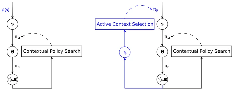
the upper-level policy πω are learned to maximize J(ω) directly. An illustration of the
components of contextual policy search is given in Figure 1.
We define the learning progress at timetwhen performing a trial in contexts, with the control policy parameters θ selected according to πω, as ∆s(t) =J(ωt+k)−J(ωt), where
ωt are the parameters learned by contextual policy search at time t. Note that contextual
policy search methods like C-REPS typically do not update ωafter every rollout but only after a certain number of rollouts k. Hence, it is more appropriate to define the learning progress over the window kthan between successive values of J(ωt).
The learning task on the task-selection level can now be framed as finding πβ such
that πβ selects contexts that maximize the expected learning progress Eπω{∆s(t)}. The
θ s
r( , )s θ
πω
πθ
Contextual Policy Search Active Context Selection
rβ
πβ
θ s
r( , )s θ
πω
πθ
Contextual Policy Search p( )s
Figure 1: Contextual policy search (left): A context vector s is given by the environment according to some fixed distribution p(s), the upper-level policy πω(θ|s)
gener-ates the parameters of the control policy for s, the control policy is executed in the environment and a reward r(s,θ) is obtained. A contextual policy search component updates the upper-level policy based on the reward with the goal to maximizeJ(ω). Active contextual policy search (right): The context vector sis selected by the context selection policy πβ which will be adjusted by an active
context selection component based on the intrinsic reward rβ. rβ is an estimate
of the learning progress based onr(s,θ). Differing parts are marked in blue.
stochastic, hence the expectation. Furthermore, the learning progress is also non-stationary since it depends on the quality of ωt: if J(ωt) is already close to the optimum, the typical
learning progress is smaller than the learning progress at the beginning of learning when
ωt is usually far from optimal.
We restrict ourselves to cases in which πβ can only select among a finite number K
of predetermined contexts {s1, . . . ,sK} during learning. These K predetermined contexts
are, however, elements of a continuous context space S over whichπω shall generalize and
where J(ω) is evaluated. The restriction to a discrete set of training contexts allows to apply well-established multi-armed bandit algorithms. Choosing the discrete set of training contexts can be based either on domain knowledge or on simple heuristics: for instance, for low-dimensional context spaces, an equally spaced grid over the context space can be used for training. In high-dimensional context spaces this would become infeasible due to the course of dimensionality. Hence, in this situation sampling the set of training contexts from a uniform random distribution over the continuous context space is more viable.
3.2 Intrinsic Reward Functions
Since Eπω{∆s(t)} is unknown to the agent and difficult to estimate because of its
non-stationarity, we propose several heuristic but easily computable reward functionsrβ which
experiments, we evaluate whichrβ is a good proxy for the actual expected learning progress.
Note that the heuristics that we propose are not exactly comparable to any query strategy from supervised learning since the learning process in reinforcement learning in a specific task is iterative unlike in typical supervised learning settings.
In a generalized form, we can write the proposed proxies of the learning progress as
rβ =f(r(st,θt)−ˆbst),
where r(st,θt) is the return obtained in episode t with policy πθt in context st, ˆbst is a baseline term, and f is an operator. Note that the bandit algorithm addresses the stochas-ticity in r(st,θt) and, hence, the heuristics usually need not account for this stochasticity
themselves.
3.2.1 Best-Reward Heuristic
This heuristic directly uses the reward obtained by the control policyπθ in tasksin rollout
tas the proxy for the learning progress, that isrβ =r(s,θt). Thus ˆbst = 0 and the operator f is simply the identity. This heuristic corresponds to assuming that the agent makes the most progress when it focuses on improving its performance in tasks in which it is already performing well. The idea behind this heuristic is that we should first learn easy tasks perfectly because this can help us to learn similar but more difficult tasks later on.
A potential problem of this heuristic are settings in which high reward does not corre-spond to easy tasks, for instance when the maximum achievable reward differs in different context. Additionally, the best-reward heuristic requires that knowledge can be transferred very well between contexts. Otherwise it converges to the context with the highest rewards.
3.2.2 Diversity Heuristic
Quite opposite to the best-reward heuristic, this heuristic encourages to select tasks in which the agent receives the worst reward. For this, the negative actual reward rβ = −r(s,θt)
is used. Thus ˆbst = 0 and the operator f is simply f(x) = −x. The intuition for this heuristic is that one should focus on the hardest tasks in which the current performance is worst since in these tasks the potential for large improvements is high. This heuristic bears similarities to the heuristic proposed by Ruvolo and Eaton (2013) for supervised learning and is hence called “diversity” heuristic.
Similar to the best-reward heuristic, this heuristic might have problems in settings in which the maximum achievable reward differs in different context and thus, the obtained rewards might not be comparable. Another disadvantage appears in cases with unlearnable contexts. The diversity heuristic would then focus on these unlearnable contexts.
3.2.3 1-step Progress Heuristic
This heuristic uses the difference of the last two rewards obtained in the respective context as proxy for the actual learning progress, that is,rβ =r(s,θt)−r(s,θ¯t), where ¯tis the index
of the previous rollout in context s. Thus the baseline is simply the last obtained reward ˆbs
Algorithm 1Discounted Upper-Confidence Bound (D-UCB) (Kocsis and Szepesv´ari, 2006)
Require: K: number of tasks; γ: discounting factor; ξ >0: some parameter controlling the strength of padding; t: number of rollouts; i1, . . . , it: previously selected tasks;
r1, . . . , rt: previous rewards
1: if t < K then
2: return t # Sample each task at least once 3: else
4: for i∈ {1, . . . , K} do
5: ni←Ptt
j=1γ
t−tj1
{itj=i} # Discounted number of rollouts in taski
6: end for
7: n←PKi=1ni # Discounted total number of rollouts 8: for i∈ {1, . . . , K} do
9: ri← n1
i Pt
tj=1γ
t−tjr
tj1{itj=i} # Discounted mean reward in task i
10: ci ←2B q
ξlogn
ni # Padding function for taski
11: end for
12: return arg maxi∈{1,...,K}ri+ci # Select task in which discounted UCB is maximal
13: end if
sandθ inJ(ω) by single samples and uses the reward sampler(s,θt) as estimate forRs,θt. As it is based solely on differences of rewards rather than absolute values, it should be able to cope better than the best-reward and diversity heuristic with situations, in which the maximum achievable reward differs in different contexts.
A drawback of the 1-step progress heuristic is that it generates reward signals rβ with
high variance. Variance inrβ is inevitable because of the stochasticity of both the
environ-ment and the upper-level policyπω. However, since the baseline of this heuristic is the last
obtained reward, this baseline has also a high variance, which need not be the case.
3.2.4 Monotonic Progress Heuristic
Although bandit algorithms account for the stochasticity in the 1-step progress heuristic, it might be useful to reduce already the variance of the intrinsic reward. We can use more stable baselines such as the maximum reward of all previous rollouts in the contexts, that is: ˆbs = max
t:st=s
r(s,θt). Furthermore, since the learning progress is typically monotonically
increasing, using the operatorf(x) = max(0, x) to avoid negative rβ appears to be
reason-able. The resulting heuristic is denoted as “monotonic progress heuristic” and has the form rβ = max(0, r(s,θt)− max
t:st=s
r(s,θt)).
The heuristic considers the learning progress to be monotonic and strictly positive. In comparison to the 1-step progress heuristic, the intrinsic reward rβ will be more often zero
3.3 Learning Context Selection Policies
Since the reward rβ is stochastic, we propose to use a learning algorithm for determining
πβ. As we consider only a finite number of predetermined contexts, the problem of learning
πβ can be framed as a MABP, where the contexts correspond to the “arms” and rβ to
the bandit’s reward. Due to the non-stationarity of rβ, standard UCB-like algorithms
are not sufficient as they expect the rewards to be drawn from a non-changing probability distribution. In contrast, we propose to use D-UCB (see Algorithm 1; Kocsis and Szepesv´ari, 2006) for active context selection since it explicitly addresses changing reward distributions. For this, D-UCB estimates the instantaneous expected reward by a weighted average of past rewards where higher weight is given to recent rewards. More specifically, a discount factor γ ≤ 1 is introduced and the reward that has been obtained at time step tj is weighted
with the factor γt−tj at time t. The central idea of D-UCB is that the discounting can compensate for continuously but slowly changing reward distributions.
The upper confidence bound of the D-UCB algorithm for arm i takes the form ri+ci
where ri = n1i Pttj=1γ
t−tjr
tj1{itj=i} is the discounted mean and ci = 2B q
ξlogn ni is the padding function which controls the width of the confidence intervals. In this formulas, ni corresponds to the discounted number of draws of arm i and n to the total discounted
number of draws (see Algorithm 1). Furthermore, rtj is the reward obtained in the tj-th rollout anditj is the arm played in this rollout. 1{itj=i} is the Kronecker delta which is one if the equality holds and zero otherwise. B and ξ are parameters of the algorithm which control the width of the confidence intervals, where B is an upper bound on the rewards and ξ needs to be chosen appropriately.
4. Model of the Contextual Learning Problem
In this section, we show how contextual policy search algorithms can benefit from active context selection by means of a simple artificial model of the contextual learning prob-lem. The model abstracts away the contextual policy search which is possible because our approach treats it as a black box (see Figure 1).
We assume that the context space S = {0,1, . . . ,9} is discrete and associated to each contextsis a hidden value ls∈[0,100] that indicates the agent’s competence in s, that is,
how wellshas been learned. Large values oflssimulate that the current policy parameters
in context sare close to the optimal policy parameters θ∗(s). The true reward in context
s, which is given by
r(s) = (1 + exp(−0.1ls+ 4))−1+bs,
depends directly on ls. r(s) corresponds to a scaled and shifted logistic function so that
r(s) ≈ bs if ls ≈ 0 and r(s) ≈ 1 +bs if ls ≥ 100. In real learning problems, different
tasks often have a different maximum reward. To simulate this, we artificially create a true reward baseline bs for each context. The baseline is randomly sampled from a normal
distribution with zero mean and standard deviation σb. The true reward is not observed
directly. Instead, we add Gaussian noise with zero mean and standard deviation σr to
simulate trial and error of a learning agent.
−2
−1 0 1 2 3 4
J
−
JRR
(a)σr= 0.00,σb= 0.00 (b)σr= 0.01,σb= 0.00
0 200 400 600 800 1000
Episode
−2
−1 0 1 2 3 4
J
−
JRR
(c)σr= 0.00,σb= 0.20
0 200 400 600 800 1000
Episode (d)σr= 0.01,σb= 0.20
Jopt
1-step Progress Best Reward Diversity
Monotonic Progress Round Robin SAGG-RIAC
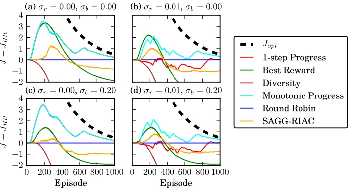
Figure 2: Relative learning curves of several active context selection methods. The perfor-mance of the round robin context selection baseline (JRR) is subtracted from all
learning curves. The values of the standard deviation for reward measurements σr and of the standard deviation for the baselineσb have been varied. After 1000
episodes the monotonic progress heuristic has approximately reached the upper bound of the performanceJopt.
neighboring contexts even in continuous domains. This model is motivated for instance by reaching tasks, in which it might happen that a slight modification of the goal position requires that the agent needs to avoid an obstacle that blocks the direct path. As a result, the slightly different context corresponding to the blocked goal would have a significantly worse expected learning progress than its neighbors and its solution cannot be transferred well. We model this behavior of learning progress and skill transfer by assigning a different learning progress factor ws∈ {0.12,0.22, . . . ,12} to each context randomly, where largews
corresponds to a larger improvement of competence after one additional trial ins.
Each time, the reward of a context st will be queried, the values ls of each contextss
will be updated to simulate the learning progress according to the update rule
ls(t) =ls(t−1)+wst·0.5|
s−st|,
which models that experience obtained in one context generalizes to other contexts based on their similarity (measured here using the euclidean distance). Contexts which are easier learnable (large ws) lead to higher overall learning progress at the beginning. However, it
does not make sense to focus at the context with maximum ws indefinitely because r(s)
saturates once ls ≥ 100. Hence, the estimate of the learning progress has to be adaptive.
Since we only have a discrete set of contexts, we can exactly compute J =P
sr(s) and the
upper bound ofJ is Jopt= 10 +Psbs.
0 200 400 600 800 1000 Episode 0 1 2 3 4 5 6 7 8 9 Selected context SAGG-RIAC
0.0 0.5 1.0 Learnability
0 200 400 600 800 1000 Episode 0 1 2 3 4 5 6 7 8 9 Selected context Monotonic Progress
0.0 0.5 1.0 Learnability
0 200 400 600 800 1000 Episode 0 1 2 3 4 5 6 7 8 9 Selected context SAGG-RIAC
0.0 0.5 1.0
ws
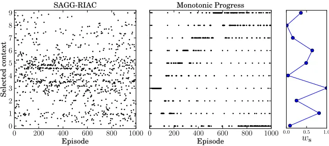
Figure 3: Selected contexts per episode with SAGG-RIAC and monotonic progress heuristic and D-UCB (with σr = 0). The learning progress factor ws of each context is
displayed on the right side.
show different properties of the active context selection methods, we display the number of episodes versus the relative J in comparison to round robin selection in Figure 2. We have used the parametersγ = 0.95 andξ = 10−8 in all heuristics that are based on D-UCB. For the diversity and the best-reward heuristics we have usedB = 1 and for all othersB = 0.25. For SAGG-RIAC, we set the maximum size of samples per region before we split the region to 8 and the window size which is used to compute the interest value is 10.
We can see that despite different learning progress factors, round robin context selection is a good baseline. The best-reward heuristic that focuses on the best learnable context is a good heuristic at the beginning. However, when the best context approaches the optimum reward, the learning progress decreases and approaches zero. At this time it would be better to switch to a context in which greater learning progress can be achieved. This will be even more significant for larger context spaces because the transferability of knowledge decreases with the size of the context space and the complexity of the different contexts. In addition, an artificial baseline for each reward (see Figure 2 (c) and (d)) leads to severe degradation because the context with maximum r(s) is not necessarily the context with maximum learning progress. The diversity heuristic does not work well either. This is because the differences of the expected learning progress are too large between contexts and it will select the worst learnable context.
The 1-step progress heuristic and monotonic progress heuristic essentially focus on the same context as the best-reward heuristic at the beginning. But they switch to other contexts with greater learning progress when the learning progress in the best learnable context decreases. Moreover, the 1-step progress and monotonic progress heuristics are invariant under different baselines. The heuristics behave identically when the reward is noise-free, that is σr = 0. If there is noise (which simulates the exploration of the agent),
the monotonic progress heuristic is usually better (see Figure 2 (b) and (d)).
learning progress: we assume that the expected learning progress of neighboring contexts can change abruptly. This is a a problem for SAGG-RIAC because it focuses on regions of the context space that have a high reward derivative. Among these are not only regions with a high learning progress but also regions with abruptly changing learning progress. In Figure 3 we can see which contexts have been selected by SAGG-RIAC during the simulated learning process: it focuses most of the time on the region around the contexts 3, 4 and 5 because of the greatly varying learning progress factorws in this region, which results in a
high competence derivative. Therefore, a significant part of the explored contexts are not informative because the context 4 has a very low learning progress.
The monotonic progress heuristic, in contrast, selects most of the time tasks with a high learning progress as we can see in Figure 3. At the beginning, it focuses on the context 3 which has the highest ws. After some time, when the learning progress in this context
saturates, it concentrates on other contexts. At the end it concentrates on the contexts that have not been learned perfectly yet even though they have a low intrinsic learning progress factor.
5. Results
We provide an empirical evaluation of the proposed methods on an artificial contextual benchmark problem in Section 5.1 and in two ball throwing tasks with a simulated Mit-subishi PA-10 in Section 5.2.
5.1 Contextual Function Optimization
In this section, we evaluate the proposed approach on an artificial test problem, compare it to reasonable baseline methods, and analyze the effect of different intrinsic reward heuris-tics. The test problem is chosen such that some contexts are harder in the sense that the parameters θ need to be chosen more precisely to reach the same level of return. By fo-cusing on learning primarily the parameters θ for these contexts, active context selection should be able to outperform a uniform random context selection.
5.1.1 Problem Domain
The context is denoted by s∈S= [−1,1]ns. We use the objective function
f(θ,s) =−||Aθ−s||2· ||s||22+
ns−1 X
i=0 si,
where θ ∈ Rnθ denotes the low-level parameters and the matrix A ∈[0,1]nθ×ns is chosen uniform randomly such that it has rank ns (nθ > ns). The objective function consists of
three terms: theparameter error −||Aθ−s||2which can be influenced by the agent’s choice
of θ, thecontext complexity ||s||2
2, which controls how strongly the agent’s parameter error
deteriorates the task performance, and thebaseline Pns−1
i=0 si, which controls the maximum
value in a context. Since A has rank ns, θ can always be chosen such that the parameter
error becomes 0 and thus the optimal valuef∗(s) is equal to the baselinePns−1
i=0 si. However,
0 500 1000 1500 2000 2500 Rollouts
−6
−5
−4
−3
−2
−1 0
Log-Cost
Best-Reward Diversity 1-Step Progress Monotonic Progress Corners Random
Figure 4: Learning Curves of Different Task Selection Heuristics. A contextual upper-level policy has been learned using C-REPS for different active task-selection strategies. The logarithm of the cost|f(θ,s)−f∗(s)|averaged over 100 test contexts is used as performance measure. Shown are mean and standard error of the mean for 20 runs of 2500 rollouts.
be considerably smaller than f∗, while the difference will be less pronounced in contexts with lower context complexity. Most extremely, fors=0, the choice ofθ is arbitrary since f will always be equal to f∗. Thus, an agent should focus on learning θ in the contexts with high complexity if its objective is to minimize |f(θ,s)−f∗(s)|.
5.1.2 Comparison of Task Selection Heuristics
In a first experiment, we compare task selection with D-UCB for different intrinsic reward heuristics to two baseline methods. In this experiment, training takes place on 25 contexts placed on an equidistant grid over a context space withns= 2 dimensions; that is, the set of
contexts that will be used for training isStrain= [−1,−21,0,12,1]2. The objective of learning,
however, is to generalizeπω over the entire context spaceS, that is, to chooseπω(θ|s) such
that f(θ,s) is maximized. As baseline, we use a “Random” task-selection heuristic, which selects uniform randomly among the training contexts. Moreover, we use a “Corner” task-selection heuristic, which selects the four contexts, where the context complexity is maximal, that is s= (±1,±1), in a round-robin fashion.
For the D-UCB, we have used B = 1.0, γ = 0.99, and ξ = 10−8. The external reward r(s,θ), based on which the intrinsic rewardrβ is computed, is set tor(s,θ) =f(θ,s) where
θ = πω(s) is sampled from the upper-level policy for the given context s. Note that the
rewards in s have high variance because of the agent’s explorative behavior and are also non-stationary since they depend on the current upper level policy πω. Contextual policy
search was conducted with C-REPS with= 2.0,N = 50, and performing an update every 25 rollouts. The evaluation criterion is the expected value of |f(πω(θ|s),s)−f∗(s)|of the
learned contextual policyπω over the context spaceS, where exploration ofπω is disabled.
We approximate this quantity by computing the average return ofπω on 100 test contexts
−1.0
−0.5 0.0 0.5 1.0
Context
sy
Best-Reward Diversity 1-Step Progress
−3.0
−2.7
−2.4
−2.1
−1.8
−1.5
−1.2
−0.9
−0.6
−0.3 0.0
Log-Selection
Ratio
−1.0−0.5 0.0 0.5 1.0 Contextsx −1.0
−0.5 0.0 0.5 1.0
Context
sy
Monotonic Progress
−1.0−0.5 0.0 0.5 1.0 Contextsx
Corners
−1.0−0.5 0.0 0.5 1.0 Contextsx
Random
−3.0
−2.7
−2.4
−2.1
−1.8
−1.5
−1.2
−0.9
−0.6
−0.3 0.0
Log-Selection
Ratio
Figure 5: Task preferences of different task-selection strategies during the first 250 rollouts of training. Shown is the logarithm of the mean selection ratio.
Figure 4 shows the learning curves for different task-selection strategies. Figure 5 shows which contexts (tasks) are selected by the different strategies during the first 250 rollouts of training. D-UCB with the “Best-Reward” and the “Diversity” intrinsic reward performs significantly worse than a uniform random task selection. The reason for this is that “Best-Reward” focuses mostly on tasks where the baseline term is large (upper-right area in Figure 5) or where the task complexity is small (central area). Conversely, “Diversity” focuses on areas where the baseline term is small. Both strategies are too imbalanced if the baseline term’s contribution is not negligible.
D-UCB with the “1-step Progress” intrinsic reward performs equally bad during the first 250 rollouts. The reason for the low initial progress is that the “1-step Progress” intrinsic reward not only rewards progress but also penalizes regression. However, regression is inevitable during the initial explorative phase. Because of this, this intrinsic reward heuristic focuses initially on contexts with small context complexity where the parameter error and thus the explorative behavior have only a small effect on the actual reward. After the initial explorative phase, this intrinsic reward gets more informative and the corresponding active task selection outperforms uniform random task selection in the long run.
D-UCB with the “Monotonic Progress” intrinsic reward performs considerably better than both D-UCB with the other heuristics and uniform random task selection. The reason for this is that it initially favors complex contexts (the outer areas in Figure 5 with||s||2
−9
−8
−7
−6
−5
−4
−3
−2
−10
Log-Cost
Context Dimensions: 1 Context Dimensions: 2
0 1000 2000 3000 4000 5000 Rollouts
−9
−8
−7
−6
−5
−4
−3
−2
−1 0
Log-Cost
Context Dimensions: 3
0 1000 2000 3000 4000 5000 Rollouts
Context Dimensions: 4
DUCB
Random (continuous) Random (discrete)
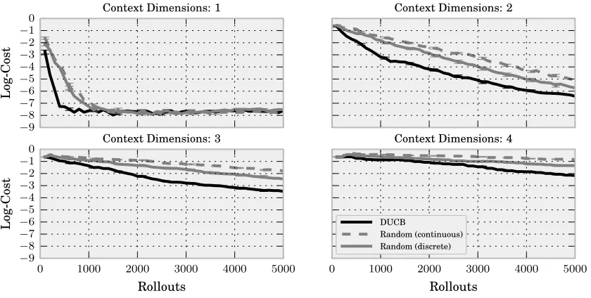
Figure 6: Learning Curves for Different Context Dimensionality. Shown are mean and standard error of the mean for 20 runs of 5000 rollouts.
suboptimal and unstable in the long run since only four of the tasks are ever sampled. Conversely, the “Monotonic Progress” intrinsic reward leads to a more balanced selection of tasks when converging and is thus favorable in the long run. In summary, D-UCB with the “Monotonic Progress” intrinsic reward selects tasks in a way which increased C-REPS’ learning progress considerably and proved to be stable at the same time.
5.1.3 Dimensionality of the Context Space
In a second experiment, we compare the performance of D-UCB to uniform random task selection for different dimensionality of the context space. A discrete setStrainof 25 contexts
for training has been generated by selecting thek-the contextskuniform random fromRns under the constraint ||sk||2 = k/25. The set of test contexts has been generated in the
same way but with an other random seed. D-UCB has been combined with the “Monotonic Progress” heuristic. The D-UCB parameters have been set toB = 1.0, γ = 0.99, and ξ = 10−8, and the C-REPS parameters to= 1.0 and N = 25n2s, and an update was performed every 13n2
srollouts. As baseline, two different random context selection strategies have been
tested: “Random (discrete)” chooses tasks uniform randomly from Strain while “Random
(continuous)”chooses tasks uniform randomly from Rns under the constraint ||sk||2 ≤1.
Figure 6 shows the learning curves for ns ∈ {1,2,3,4}. For any value of ns, D-UCB
ns, this is not directly an issue of the task-selection strategy (since D-UCB still outperforms
random task selection) but rather of the underlying contextual policy search method. Thus, the results show that active context selection with D-UCB works satisfyingly while higher dimensional context spaces remain a general challenge for contextual policy search.
5.2 Generalize Throwing Movements
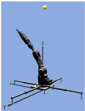
Figure 7: Visualization of the simulated Mitsubishi PA-10 throwing a ball.
In this section, we consider the problem of learn-ing to throw a ball at a given target. A similar setting has been investigated by Wirkus et al. (2012), where the objective was to learn throw-ing an object at a specified target based on a for-ward model of the system. In our experiments, the target can be located at different positions in a predetermined area on the ground and we do not provide any model of the system, making it a contextual model-free policy search problem with the target position being the context. We consider two different reward functions for this experiment. One reward function is continuous (grid problem) while the other has discontinu-ities and flat regions without a “reward gradi-ent” (dartboard problem), resulting in a setting with easy and more difficult tasks. We provide an empirical evaluation on the grid problem and apply the gained insight on the dartboard prob-lem. In our experiments, we use a simulated Mitsubishi PA-10 robot arm with seven joints for throwing (see Figure 7).
5.2.1 Policy Representation
A throwing behavior in this experiment consists of a sequence of two movement primitives (DMPs), where the first corresponds to the strike out and the second one to the actual throwing movement. Both primitives have a duration of τ1 = τ2 = 0.5 s. The movement
primitives define joint trajectories directly for the seven joints of the Mitsubishi PA-10. The parameters of the two DMPs include the weights of the forcing terms and the respective meta-parameters (see Section 2.1). These parameters have been initialized such that the resulting throw hits the ground position (−3.55,−3.55), where (0,0) is the ground position at which the PA-10 is mounted and the unit of the coordinate system is in meter. Some of the meta-parameters of the initial policy are to be adapted later on such that other ground positions are hit. These include the final state of the first movement primitive g1
and the velocities at the end of the two movement primitives ˙g1,g˙2. Instead of modifying
θ = (g1,g˙1,g˙2) directly, we use the values from the initial policy θ0 as the base and we
modify the offset t so that θt = θ0+t. The weights w of the forcing terms of the two
the actual contextual learning task consists of finding a mapping for 3·7 = 21 parameters such that different target positions on the ground are hit.
5.2.2 Methods
We use C-REPS for contextual policy search with the contextswhich contains the Cartesian coordinates of the target position for the throw. The mapping ϕ projects the context to polar coordinates and generates all quadratic terms of the polar coordinates. This mapping results from the constraint of C-REPS to match feature averages instead of the actual context distribution, which would result in an infinite number of constraints (Deisenroth et al., 2013). A policy update is performed after every 50 trials and a memory of at most 300 trials is used for the update. This memory consists of the best 300/K trials for each of theK tasks, which results in an update that is similar to importance sampling in PoWER (Kober and Peters, 2011). We restricted the maximum Kullback-Leibler divergence of the old and new policy distributions to = 0.5, the initial weight matrix was set to W = 0, and the initial covariance was set toΣ=σ20I withσ20 = 0.02. For D-UCB, we useγ = 0.99, B = 10,000 and ξ= 10−9 in all cases.
5.2.3 Grid Problem
We define two contextual learning problems in this setting whose main difference is the structure of the reward function. The first reward function provides the squared distance of the position hit by the throw to the target position as reward: r(s,θ) = −||s−bθ||22,
where s is the target and bθ are the Cartesian coordinates of the ball when it hits the
ground after executing policy πθ. In this problem, we generate an equidistant grid of 25
targets for training over the area [−3,−5]×[−3,−5]. Another set of 16 targets is used to test the generalization. These targets form an equidistant grid in the area [−3.25,−4.75]× [−3.25,−4.75]. While different contexts share the same reward function, learning them might differ in complexity. Some of the relative positions of the target to the PA-10 arm are harder to hit because of the kinematic structure of the arm. In addition, the distance to the initial policy makes some contexts easier to solve by exploration than others.
We compared our methods to three baselines: continuous random sampling of contexts from [−3,−5]×[−3,−5] (“Random (cont.)”), selection in a fixed order (“Round Robin”) and the best policy that we have found in all experiments (“Best Policy”). On the left side of Figure 8 the learning curves of several intrinsic reward heuristics are shown and on the right side the best intrinsic reward heuristic is compared to the baselines.
Best Policy Best-Reward Diversity
1-step Progress Monotonic Progress
Round Robin Random (cont.)
0 2000 4000 6000 8000 10000
Episode
0 10 20 30 40 50 60 70 80 90 100
Distance
to
test
targets
(cm)
0 2000 4000 6000 8000 10000
Episode
0 10 20 30 40
Figure 8: Left: Learning curves of several intrinsic reward heuristics for D-UCB in the grid problem. We measured the average distance to the test targets. The curves and the error bars show the mean and standard error of mean over 20 runs. “Best Policy” indicates the performance of the best policy that we have generated in all experiments. Right: Comparison of D-UCB with intrinsic reward based on the monotonic progress with the baselines.
the tasks in which one can make the greatest estimated learning progress gives a significant advantage in this problem. In contrast to the results in Section 5.1, the “1-step Progress” heuristic is on a par with the “Monotonic Progress” heuristic. A possible reason for this is that the inherent context complexities in this task do not vary as strongly as in the problem in Section 5.1.
In comparison to the baselines, D-UCB under the monotonic progress intrinsic reward is on a par with round robin selection and slightly worse than continuous random selection. Continuous random sampling learns more quickly in the beginning because the comparison of different methods is done on a set of test contexts that are maximally dissimilar from the discrete training context set. Methods that use only the discrete set of training con-texts during the training phase have thus a disadvantage compared to continuous random sampling which typically samples closer to the test contexts.
Bull
Inner circle
Outer circle
Treble
Double
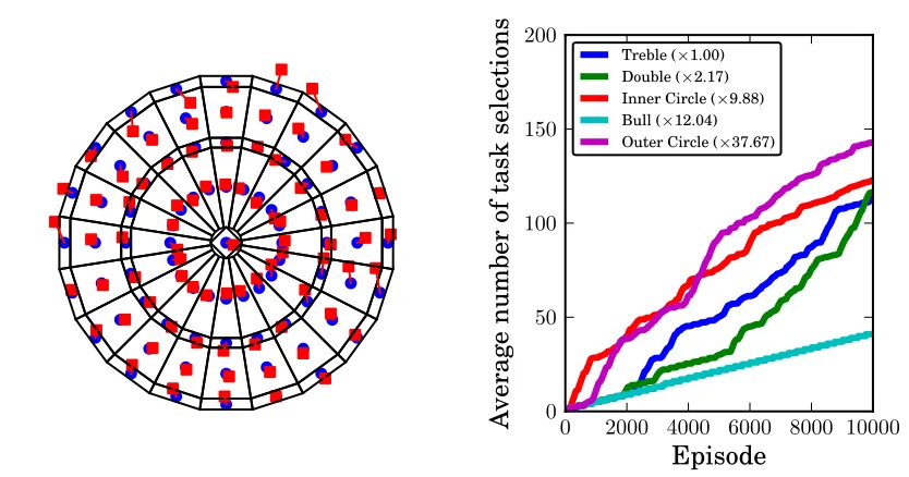
Figure 9: Left: The dartboard is divided into 81 quadrangular fields. Bull and bull’s eye are regarded as one field, the rest belongs to one of the four circles (inner circle, outer circle, doubles, and trebles). The initial policy given by θ0 would throw
at the center of the dartboard, that is the bull. Right: The target regions of the bull, inner circle, and outer circle are greater than the corresponding fields on the dartboard and overlap neighboring fields. Shown here are 5 of the 20 target regions of the inner circle. These target regions are only used to compute the reward. Larger target regions can be assumed to make the corresponding learning tasks easier.
namely to keep a separate history of samples per context of identical size (300/K rollouts per context), because it does not encounter any context twice.
5.2.4 Dartboard Problem
As second scenario with the PA-10, we consider a problem which poses tasks of more significantly varying complexity onto the agent. The targets are designed to correspond to the fields on a dartboard. This virtual dartboard is placed on the ground in front of the PA-10. Placing the dartboard on the ground instead of a wall was mainly done to simplify implementation. The diameter is set to 1.4 m (real dartboards have a diameter of 0.451 m). Each field is approximated by quadrangles (see Figure 9) and the center of this field is the context of the task corresponding to the field. For each target, we assign a corresponding
target area which is usually the quadrangular field. For some tasks, we enlarge each side of the quadrangular field by the factor 3.5 to build the corresponding target region (see Figure 9 for details). This will make these tasks considerably easier than others. The reward function gives a constant negative reward outside of this target area and only provides a reward gradient inside of the target area. The reward function is defined as
r(s,θ) =
(
−10ds,000||s−bθ||2 ifbθ is within the target area of s
−10,000 otherwise ,
0 2000 4000 6000 8000 10000
Episode
0 50 100 150 200
A
verage
number
of
task
selections
Treble (×1.00) Double (×2.17) Inner Circle (×9.88) Bull (×12.04) Outer Circle (×37.67)
Figure 10: Left: Final upper-level policy. The blue circles mark the center of each field, the red squares that are connected to the corresponding centers with a red line show the position at which the robot arm has actually thrown the ball. Right: Accumulated average number of selections for different task categories. Larger target areas and target areas that are closer to the initial policy are selected more often at the beginning. The relative size in comparison to the smallest target region is given in brackets in the legend.
to the grid setting as no reward gradient helps the agent in improving its policy if it does not hit the target area, within which a reward gradient guides the agent to the center of the field. Thus, the tasks corresponding to larger fields can be considered to be easier since it is more likely that the agent finds a reward gradient during the initial exploration. The agent should thus focus first on these tasks and select the more difficult tasks not until it has improved its contextual policy so far that it is able to hit the corresponding target areas.
We trained with all 81 targets for 50,000 trials and use the monotonic progress intrinsic reward. The result is displayed in Figure 10: the learned policy hits the “bull”, 18 of 20 fields in the inner circle, 15 of 20 trebles, 20 of 20 fields in the outer circle, and 9 of 20 doubles. The overall mean error is 4.62 cm, the median error is 3.77 cm, and the maximum error is 15.96 cm.
Doubles are the most difficult tasks to learn for the agent because they are far away from the initial policy, the target region is small and we cannot transfer much knowledge from neighboring tasks, because they are on the edge of the dartboard. For this reason, some doubles have not been learned very well. In contrast, the trebles can be learned easily, because the solution can be obtained approximately by transferring the solutions of neighboring fields from the inner circle and the outer circle.
regions are selected most often in the beginning. The targets from the inner circle are selected even more often than the targets from the outer circle during the first 1,000 episodes even though they are considerably smaller. This is because they are more likely to be reached when exploring from the initial policy which throws at the center of the dartboard. For the same reason trebles are selected more often than doubles at the beginning. After this initial phase, the fields of the outer circle are selected more often because they are now much easier to learn. The bull is so rarely selected because the initial policy will already generate a very good result for this context, hence, improvement is hardly possible.
6. Conclusion and Outlook
We have considered the problem of active task selection in contextual policy search. The hypothesis investigated in this paper is that learning all tasks with the same priority in a round robin or random fashion is not always optimal, in particular if the tasks have different characteristics which make some of them more difficult than others. We have proposed an active task-selection heuristic based on the non-stationary bandit algorithm D-UCB which learns to select tasks that have a large intrinsic reward. These intrinsic rewards can be considered as proxies for the actual learning progress which encourage the agent to engage in those tasks in which its performance is increasing the most. The underlying model of the learning process assumes that each task has a different intrinsic expected learning progress which might change abruptly in the context space and that knowledge can be transferred between neighboring contexts.
Our empirical results have shown that active task selection can make a considerable difference for the learning speed of contextual policy search. In general, we found that a task-selection method should explore in the beginning, then focus on several easy tasks to acquire some initial procedural knowledge, thereupon transfer knowledge to similar but more difficult tasks, and concentrate in the end on those tasks that have not been learned yet. Some of the proposed intrinsic reward heuristics provide a considerable advantage over round robin or uniform random selection in our empirical evaluations on a contextual function maximization problem and a simulated robotic ball throwing experiment.
We restricted ourselves to a discrete set of context vectors for training. In the future it would be interesting to explore not only a discrete set of tasks but a continuous range of task parameters such as arbitrary rather than grid-based target positions for ball throwing as in Section 5.2.3. This could be modeled as a non-stationary continuum-armed bandit problem. However, the non-stationary version of the continuum-armed bandit problem (Agrawal, 1995a) has not been explored thoroughly yet.
The goal of the proposed method is to reduce the wear and tear of (possibly robotic) agents as well as the human intervention during learning. Selecting the context actively typically requires some mechanism that sets the environment in the requested context. To limit the amount of human intervention, it is very desirable that the agent can set the desired context on its own. This is typically trivial in simulation. In real-world problems, it can often be achieved by means of previously learned or hard-coded skills. In case that a human supervisor needs to produce the requested context, the feasibility of active context selection depends on the amount of work imposed on the human supervisor and thus, on the specific task.
Among the kind of tasks for which we consider active contextual policy search to be promising are: various kind of goal-directed reaching, hitting and throwing problems like for example ball throwing, darts and hockey. Moreover, scenarios in which an agent can select from a small set of predefined contexts, for example grasping one object from a set of objects with varying size and shape, are promising. Another scenario could be that a robot has to learn how to walk on a restricted set of different terrain surfaces, where the context consists of the properties of the surfaces.
In the future, within the research we will conduct in the context of the project “Be-haviors for Mobile Manipulation” (BesMan),2 we plan to evaluate the proposed approach
on different robotic target platforms, among others the humanoid robot AILA. One of the challenges for this is to bridge the simulation-reality gap: multiple executions of the same policy often have significantly different outcomes on actual robots like AILA due to different initial states and other unobserved properties. Thus, the learning approach needs to be able to deal with noise in the executions.
Acknowledgments
This work was supported through two grants of the German Federal Ministry of Economics and Technology (BMWi, FKZ 50 RA 1216 and FKZ 50 RA 1217). In particular, we would like to thank Yohannes Kassahun for helpful comments.
Appendix A. Implementation of Contextual REPS
Contextual relative entropy policy search has been explained in detail by Deisenroth et al. (2013) and Kupcsik et al. (2013). We summarize C-REPS in Algorithm 2. A stochastic policyπω(θ|s) is used to generate low-level controllersπθ for a contexts. In this paper, we
use a Gaussian policy with linear mean (Deisenroth et al., 2013) so thatω= (W,Σ). After collecting N experience tuples (si,θi, r(si,θi)) (lines 2-6), C-REPS determines a weight
di for each experience based on the context-dependent baseline V(s) = vTϕ(s) (lines
7-10). With the obtained weights, C-REPS updates the policy through weighted maximum likelihood (lines 11-17).
Implementing C-REPS is not straightforward. In our experiments and for our reward functions it was sometimes numerically unstable. To improve the reproducibility of the
Algorithm 2 Contextual relative entropy policy search (C-REPS)
Require: : maximum Kullback-Leibler divergence between two successive policy distri-butions;ϕ(s): extracts features from the context s;N: number of samples per update;
W: initial weights of upper level policy; Σ: initial covariance of upper level policy distribution
1: whilenot convergeddo 2: for i∈ {1, . . . , N} do
3: Select contextsi # For example, based onsome specified task-selection method
4: θi∼ N(WTϕ(si),Σ) # Draw policy parameters
5: Obtainr(si,θi) # Return of policy πθi in environment with contextsi 6: end for
7: Solve constrained optimization problem [η,v] = arg minη0,v0g(η0,v0), s.t. η >0
g(η,v) =η+vTϕˆ+ηlog
N
X
i=1
1 N exp
r(si,θi)−vTϕ(si)
η
!
8: for i∈ {1, . . . , N} do
9: di ←exp
r(si,θi)−vTϕ(si)
η
# Determine weight for each experience tuple 10: end for
11: for i∈ {1, . . . , N} do# Prepare policy update 12: Φi =ϕ(si)T
13: Θi=θTi
14: end for
15: D =
d1
0
. ..
0
dN
16: Wnew←(ΦTDΦ)−1ΦTDΘ# Update policy mean 17: Σnew←
P idi (P
idi)2−Pid2i
(Θ−ΦW)T D(Θ−ΦW)# Update exploration covariance 18: end while
results, we explain some of the modifications that we had to make in addition to the log-sum-exp trick (in line 7) that is already mentioned by Deisenroth et al. (2013).
The weighted least squares problem is sometimes ill-conditioned. Hence, we added the regularization term λI so that
Wnew←(ΦTDΦ+λI)−1ΦTDΘ.
In our experiments, we useλ= 10−4.
At the end of the learning process, η sometimes becomes very small which causes nu-merical problems. It is helpful to use an other lower bound ηmin, so that η > ηmin, for
exampleηmin ∈(10−6,10−4).
For very large negative rewards the weights di are sometimes so small that they cannot
softmax-like term
di=
di
P
jdj
=
expr(si,θi)−vTϕ(si)
η
P
jexp
r(s
j,θj)−vTϕ(sj)
η
,
which does neither change the weights of the linear policyWnew, nor the covarianceΣnew.
Softmax can be implemented numerically stable:
di=
expr(si,θi)−vTϕ(si)
η
P
jexp
r(s
j,θj)−vTϕ(sj)
η
=
expr(si,θi)−vTϕ(si)
η −m
P
jexp
r(s
j,θj)−vTϕ(sj)
η −m
,
wherem= max
i
r(si,θi)−vTϕ(si)
η .
In addition, for the experiments in Section 5.2 we use a kind of importance sampling to reuse experience tuples from previous rollouts: for every task we maintain a memory of the best N/K rollouts, where N is the maximum number of samples for a policy update and K is the number of tasks. Note that this might have a negative effect if there are multiple local optima that are separated by regions with low return in some contexts.
References
Rajeev Agrawal. The continuum-armed bandit problem. SIAM Journal on Control and Optimization, 33(6):1926–1951, 1995a.
Rajeev Agrawal. Sample mean based index policies with O(log n) regret for the multi-armed bandit problem. Advances in Applied Probability, 27(4):1054–1078, 1995b.
Adrien Baranes and Pierre-Yves Oudeyer. Active learning of inverse models with intrin-sically motivated goal exploration in robots. Robotics and Autonomous Systems, 61(1): 49–73, 2013.
Andrew G. Barto, Satinder Singh, and Nuttapong Chentanez. Intrinsically motivated learn-ing of hierarchical collections of skills. InProceedings of the 3rd International Conference of Developmental Learning, pages 112–119, LaJolla, CA, USA, 2004.
Yoshua Bengio, J´erˆome Louradour, Ronan Collobert, and Jason Weston. Curriculum learn-ing. In Proceedings of the 26th International Conference on Machine Learning, pages 41–48, 2009.
S´ebastien Bubeck and Nicol`o Cesa-Bianchi. Regret analysis of stochastic and nonstochastic multi-armed bandit problems. Foundations and Trends in Machine Learning, 5(1):1–122, 2012.
William S. Cleveland and Susan J. Devlin. Locally weighted regression: An approach to regression analysis by local fitting. Journal of the American Statistical Association, 83 (403):596–610, 1988.