An Approximate Analytical Solution of Higher-Order Linear Differential Equations with Variable Coefficients Using Improved Rational Chebyshev Collocation Method

Published online December 27, 2014 (http://www.sciencepublishinggroup.com/j/acm) doi: 10.11648/j.acm.20140306.15

ISSN: 2328-5605 (Print); ISSN: 2328-5613 (Online)

An approximate analytical solution of higher-order linear

differential equations with variable coefficients using

improved rational Chebyshev collocation method

Mohamed A. Ramadan

1

, Kamal R. Raslan

2

, Mahmoud A. Nassar

2

1

Mathematics Department, Faculty of Science, Menoufia University, Shebein El-Koom, Egypt 2

Mathematics Department, Faculty of Science, Al-Azhar University, Nasr-City, Cairo, Egypt

Email address:

[email protected] (M. A. Ramadan), [email protected] (M. A. Ramadan), [email protected] (K. R. Raslan), [email protected] (M. A. Nassar)

To cite this article:

Mohamed A. Ramadan, Kamal R. Raslan, Mahmoud A. Nassar. An Approximate Analytical Solution of Higher-Order Linear Differential Equations with Variable Coefficients Using Improved Rational Chebyshev Collocation Method. Applied and Computational Mathematics. Vol. 3, No. 6, 2014, pp. 315-322. doi: 10.11648/j.acm.20140306.15

Abstract:

The purpose of this paper is to investigate the use of rational Chebyshev (RC) collocation method for solving high-order linear ordinary differential equations with variable coefficients. Using the rational Chebyshev collocation points, this method transforms the high-order linear ordinary differential equations and the given conditions to matrix equations with unknown rational Chebyshev coefficients. These matrices together with the collocation method are utilized to reduce the solution of higher-order ordinary differential equations to the solution of a system of algebraic equations. The solution is obtained in terms of RC functions. Numerical examples are given to demonstrate the validity and applicability of the method. The obtained numerical results are compared with others existing methods and the exact solution where it shown to be very attractive and maintains better accuracy.

Keywords:

Rational Chebyshev Functions, Higher-Order Ordinary Differential Equations, Rational Chebyshev Collocation Method

1. Introduction

The application of Chebyshev polynomial and rational Chebyshev collocation methods for solving different problems of differential, integro-differential equations and some other physical problems with variable, for interested readers we refer to [1,2,3]. Chebyshev polynomial approach for higher order linear Fredholm- Volterraintegro-differential equations is introduced by GamzeYüksel at el. [1]. The use of rational Chebyshev collocation method to get an approximate solution of Magnetohydrodynamic (MHD) flow of an incompressible viscous fluid over a stretching sheet is considered by SaeidAbbasbandy at el. [2]. In [3] Parand and Razzaghi introduced rational Chebyshev functions as a new computational method for solving Volterra model for population growth of a species within a closed system where the Volterra population model is first converted to an equivalent nonlinear ODE, the solution of which is then approximated by a rational Chebyshev functions with unknown coefficients.

differential equations, Rational Chebyshev tau method for solving higher-order ordinary differential equations is presented by K. Parand and M. Razzaghi [12]. In addition, M. Sezer and M. Kaynak [13] used Chebyshev polynomials for solving of linear differential equations. On the other hand, SalihYalçınbaş, et al. and M. Sezer et al. [14, 17] investigated the use of the rational Chebyshev collocation method to get approximate solution of higher order linear differential equations, respectively.

The organization of this paper is as follows. In Section 2, Preliminaries introduced while in Section 3 Properties of the rational Chebyshev (RC) functions are presented.. In Section 4, we formulated the fundamental matrix relation based on collocation Points. In Section 5, main results are presented. Section 6 contains numerical illustrations and results are compared with the exact solution. Finally, section 7 concludes this article with a brief summary.

2. Preliminaries

The rational Chebyshev collocation method presented in [17] will be developed and improved in terms of the derivatives in obtaining the fundamental matrix derivative relations of RC, and then it will be applied to solve

m

th -order linear nonhomogeneous differential equation of the form:

∑

=

= m

k

k

k x y x g x

P

0

) (

), ( ) ( )

( 0≤x<∞, (2.1)

With the mixed conditions

( )

( )

∑ ∑

−

= =

=

1

0 0

m

k J

j

i j k k ijy c

u λ , (2.2)

,

0≤c_j<∞ _{j =0,1,…,J ; i =0,1,…,m-1,}

whereP_k(x) and g(x) are continuous functions on [0,∞); , The solution of equation (2.1) and (2.2) is expressed in terms of the rational Chebyshev functions as follows:

∑

=

= N

n n nR x a x y

0

), ( )

( 0≤x<∞ (2.3)

wherea_n, n=0,1,…,N are the coefficients to be determined;

) (x

R_n , n=0,1,…,N are the rational Chebyshev functions;

i j k ij c and

u , λ are appropriate constants.

3. Properties of the Rational Chebyshev

(RC) Functions

3.1. Rational Chebyshev Functions

In the case when errors near the ends of an interval [a, b] are of particular importance, a weighting function which is of the form 1/ (x−a)(b−x)is often useful. It is supposed again

that a linear change in variables has transformed the given interval into the interval [-1, 1], so that the weighting function becomes_w

( )

_{x =1/ 1−x}2_.

In other words a great variety of other types of least – square polynomial approximation can be formulated in terms of other weighting functions. In particular, for the weighting function w

( ) ( ) ( )

x =1−xα1+xβ ,

(

α>-1,β>-1

)

over [-1, 1], which reduces to Legendre case when α=β=0 and to the

Chebyshev case when α=β=−1/2 . The well-known

Chebyshev polynomials are orthogonal in the interval [-1, 1]

with respect to the weight function

( )

2

1 /

1 x

x

w = − and can be

determined with the aid of the recurrence formulae

0( ) 1, ( )1 , n 1( ) 2 n( ) n1( ) n 1

T x = T x =x T₊ x = x T x − T₋ x ≥

The RC functions are defined byor clearly

     

+ − =

1 1 )

(

x x T x

Rn n

0 1 1 1

1 1

( ) 1, ( ) , ( ) 2 ( ) (x) , n 1

1 n 1 n n

x x

R x R x R x R x R

x + x −

−  − 

= = ₊ =  ₊  − ≥

  (3.1.1)

Rational Chebyshev functions are orthogonal with respect to

the weight function w(x)=1 ((x+1) x) in the interval

), , 0

[ ∞ with the orthogonally property:

∫

∞

=

0 2

) ( ) ( )

( nm

m m

n

c dx x w x R x

R πδ

with

2, 0 1, 1 m

m c

m

= 

=

≥ 

where

δ

_nmis the Kronecker function.

Since the set of RC functions is orthogonal and complete,

y(x) defined over the interval

[

0

,

∞

)

can be expanded as:

∑

∞

=

=

0 ), ( )

(

n n nR x

a x y

where

∫

∞

=

0

. ) ( ) ( ) ( 2

dx x w x y x R c

a i

i

i

_π

3.2. Fundamental matrix Derivative Relation of RC

The derivative of the vectorR(x)=

[

R0(x) R1(x) ... RN(x)

]

can be expressed by

) ( ) ( ) ( )

( R xD Bx

dx x dR x

R′ = = T+ (3.2.1)

improve the approximate obtained solutions as will be shown in the numerical examples section. The two D and B are deduced as shown below.

Differentiating Eq. (3.1.1) we get:

), ( ) ( 1 1 2 ) ( ) 1 ( 4 )

( _{2 1}

1 R x R x

x x x R x x

R_{n+ n}  _n′ − _n′₋

     + − + + =

′ _n≥1.

The derivative of R1(x) is 2

) 1 (

2 +

x which can be expressed

as follows: ), ( 4 1 ) ( ) ( 4 3 ) 1 ( 2 )

( 2 0 1 2

1 R x R x R x

x x

R = − +

+ = ′

Form the above; the elements dij,of the matrix D can be

obtained from

(

)

      > ′ − ′ = ′ + − = ′ = ′ −

+( ) 2 ( ). ( ) ( ), 1,

), ( 4 1 ) ( ) ( 4 3 ) ( , 0 ) ( 1 1 1 2 1 0 1 0 n x R x R x R x R x R x R x R x R x R n n n (3.2.2) where ] [ 2 1 n m n m n

mR R R

R = ₊ + ₋

The general form of the matrix D is a lower- Heisenberg matrix which can be expressed asD=D1+D2, where D1is a

tridiagonal matrix which is obtained from

, ) 1 ( 4 1 ), 1 ( ), 1 ( 4 7 . 1       − − − −

=diag i i i

D i=1,2,…,N+1

and the

d

_ij elements of matrix D are obtained from 2 d21=−1

and    − < − − ≥ = , 1 ) 1 ( 1 , 0 i j c i k i j d j ij

where ( 1) , 1 1

1 ₌ −

= + + _c

k i j and

c

_j

=

2

for

j

≥

2

.

For N =5 we have

. 5 4 / 35 10 10 10 5 1 4 7 8 8 4 0 4 / 3 3 4 / 21 6 3 0 0 2 / 1 2 2 / 7 2 0 0 0 4 / 1 1 4 / 3 0 0 0 0 0 0                   − − − − − − − − − − − = D

and

B

(x

)

is set to be of the form:

[

0 0 0 1, 2 1( )

]

1( 1)

)

( = _{+ + + × +}

N N N

N R x

d x

B ⋯

Consequently, the th

k derivative of the matrix R(x)

defined in (3.2.1), can be obtained as

1 1 0 0 ≥ + = =

∑

− = k ) D ( ) x ( B ) D )( x ( R ) x ( R ), x ( R ) x ( R 1 -i -k T k i ) i ( k T ) k ( ) ( (3.2.3) where

[

]

1( 1)

) ( 1 2 , 1 )

( _{( ) 0 0 0 ( )}

+ × + + +

= k _N

N N N

k _{x d R x}

B ⋯

4. Fundamental Matrix Relation Based

on Collocation Points

Let us first assume that the solution y (x) of Eq. (2.1) can be expressed in the form (2.3), which is a truncated Chebyshev series in terms of RC functions. Then y (x) and its derivative can be put in the matrix forms

A x R x y( )] ( )

[ = (4.1) and

A x R x

y j ( )] j ( )

[ ( ) = ( ) j=0,1,…,m≤N _(4.2)

where

[

(

)

(

)

...

(

)

]

)

(

1( ) ( )

) ( 0 ) (

x

R

x

R

x

R

x

R

Nj

j j

j

=

[

]

T

N

a

a

a

A

⋯

1 0

=

Substituting relation (4.2.3) into Eq. (5.2), we get

A

)

D

(

x

B

D

x

R

x

y

T k-i-1

k i i k T k

}

)

(

)

)(

(

{

)]

(

[

1 0 ) ( ) (

_∑

− =

+

=

(4.3)

Now, let us define the collocation points

x

_sas

, s 0,1, , s

c

x s

N

= = … _{N (4.4)}

so that 0≤x_s≤c<∞;c∈IR+.

Hence, upon substituting these points into Eq. (4.1) to obtain

∑

=

=

m k s s k s

k

x

y

x

g

x

P

0

)

(

₍

₎

₍

_);

)

(

s=0,1,2,…,N _(4.5)

The obtained system (5.5) can be written farther in the matrix form

∑

= = m k k k 0 ) ( G Y

P (4.6)

Now putting the collocation points xs, s=0,1,2,…,N,in the

relation (10) we get the system

A D x B D x R x y T k i s i k T s s k } ) ( ) )( ( { )] ( [ 1 0 ) ( ) ( ) ( k-i-1

∑

−

=

+ =

In short, we have

) ( B R

Y k-i-1

A D D T k i i k T k } ) ( { 1 0 ) ( ) (

∑

− = +

= (4.7)

where             =             = ) ( ) ( ) ( ) ( ) ( ) ( ) ( ) ( ) ( ) ( ) ( ) ( 1 0 1 1 1 1 0 0 0 1 0 0 1 0 N N N N N N

N R x R x R x

x R x R x R x R x R x R x R x R x R … ⋮ ⋱ ⋮ ⋮ … … ⋮ R             =             = ) ( ) ( ) ( ) ( ) ( ) ( ) ( ) ( ) ( ) ( ) ( ) ( 1 0 1 1 1 1 0 0 0 1 0 0 1 0 N N N N N N

N B x B x B x

x B x B x B x B x B x B x B x B x B … ⋮ ⋱ ⋮ ⋮ … … ⋮ B

Hence, from the matrix forms (4.6) and (4.7) we obtain the fundamental matrix equation for Eq.(2.1) as

∑

∑

= − = = + m k T k i i k T

k D D A

0 1 0 ) ( ; } ) (

{R B ( ) G

P k-i-1 (4.8)

Also, we obtain matrix forms corresponding the mixed conditions (2.2) as follows:

Set

x

=

c

_jin relation (4.3) we get the fundamental matrix

equation corresponding to the mixed conditions (2.2):

∑ ∑

−

∑

= = − = = + 1 0 0 1 0 ) ( } ) ( ) )( ( { m k J j i T k i j i k T j k

ij R c D B c D A

a ( )k-i-1 λ ;

i=0, 1, 2,…, m-1, (4.9)

so that 0≤cj<∞,j =0, 1,…, J.

5. Main Results

The fundamental matrix equation (4.8) for Eq. (2.1) corresponds to a system of (N+1) algebraic equations for the (N+1) unknown coefficients a₀,a₁,...,a_N.

One writes Eq. (4.8) in short form as:

) 1 . 5 ( ] ; [ G

G or W

WA=

so that

W =

∑

∑

= − = = + = m k T k i i k T k

pq D D pq N

w

0

1

0 )

( _{}; , 0,1,...,} )

( { ]

[ P R B ( )k-i-1

We can obtain the matrix form for the mixed conditions (2.2), by means of Eq. (4.9),briefly, as

, 1 ,..., 1 , 0 ] ; [U or

; _i = −

= i m

A

U_i λ_i λ_i (5.2)

where

∑∑

−

∑

= = − = + = 1 0 0 1 0 ) ( } ) ( ) )( ( { m k J j T k i j i k T j k ij

i c R c D B c D

U ( )k-i-1

Now, the solution of Eq.(2.1) under the conditions (2.2), can then be obtained by replacing the rows of matrices (5.2)by the last m rows of the matrix (5.1), we get the required augmented matrix

[ ]

. ; ; ; ; ) ( ; ; ) ( ; ) ( ; ~ ; ~ 1 , 1 1 , 1 0 , 1 1 1 11 10 0 0 01 00 , 1 , 0 , 1 1 11 10 0 0 01 00                           = − − − − − − − − m N m m m N N m N N m N m N m N N N u u u u u u u u u x g w w w x g w w w x g w w w W λ λ λ … … … … … … … … … … … … … … … …

G (5.3)

If rank W~=rank[W~;G~]=N+1,then we can write the matrix equation (5.1) as:

G~

) ~ ( −1 = W

A (5.4)

and therefore the coefficients

a

_n ; n =0, 1,…, N are uniquely

determined by Eq.(6.3)

6. Numerical Examples

In this section, numerical examples are given to illustrate the applicability, accuracy and effectiveness of the proposed technique. All examples are performed on the computer using a program written in MATHEMATICA 7.0. The obtained numerical results are presented as shown in the illustrative Tables and graphs The absolute errors,in tables, are given by the values of y(t)−y_N(t) evaluated at selected points.

Example1

Let us consider the following two point boundary value problem [12] ] 1 , 0 [ , ) 1 ( 1 ) ( ) 1 ( 1 ) ( 2

2 = ₊ ∈

+ − − ′′ x x x y x x x y with 2 1 ) 1 ( , 1 ) 0

( = y = y

For this example we have,

. ) 1 ( 1 ) ( , 1 ) ( , 0 ) ( , ) 1 ( 1 ) ( ,

2 0 2 1 2 ₂

+ = = = + − = = x x g x P x P x x x P m

Then, for N = 4, the collocation points are

1 , 4 3 , 2 1 , 4 1 ,

0 1 2 3 4

0= x = x = x = x =

x

G B B R P B R P R

P + ( DT+ )+ ( (DT) + DT+ ′)}A=

{ 0 1 2 2

whereP0, P1, P2, R, B, D are matrices of order 5×5 given, for this example, R , 4 4 3 0 0 0 7 3 2 1 0 0 8 4 21 2 4 1 0 8 6 2 7 1 0 4 3 2 4 3 0 , 1 0 1 0 1 2401 2017 343 143 49 47 7 1 1 81 17 27 23 9 7 3 1 1 625 527 125 117 25 7 5 3 1 1 1 1 1 1                           − − − − − − − − =                     − − − − − − − − − −

= _DT

, 0 0 0 0 0 16807 11041 0 0 0 0 242 241 0 0 0 0 3125 237 0 0 0 0 1 0 0 0 0 , 4 85 4 21 8 3 0 0 53 8 135 2 5 8 1 0 4 347 4 135 2 15 4 3 0 110 8 387 2 27 8 15 0 59 27 8 65 4 5 0 )2                     − − − =                           − − − − − − − − −

= B

(_DT

                =                 =                     − − − − = 1 0 0 0 0 0 1 0 0 0 0 0 1 0 0 0 0 0 1 0 0 0 0 0 1 , 0 0 0 0 0 0 0 0 0 0 0 0 0 0 0 0 0 0 0 0 0 0 0 0 0 , 0 0 0 0 0 0 49 4 0 0 0 0 0 9 2 0 0 0 0 0 25 12 0 0 0 0 0 1 2 1

0 P P

P

The augmented matrix forms of the conditions for N = 4 are

[

]

    ₋ − − 2 1 ; 1 0 1 0 1 1 ; 1 1 1 1 1

Then, we obtain the augmented matrix (6.3) as

                    − − − − − − − − − − − − = ; 2 1 ; 1 0 1 0 1 1 : 1 1 1 1 1 9 4 ; 243 2230 243 1102 81 398 9 10 9 2 25 16 ; 15625 395444 625 16716 625 7252 25 44 25 12 1 ; 383 131 31 3 1 ] ~ ; ~ [WG

we then obtain the solution for WA=G

  

 −

= 0 0 0

2 1 2 1

A

Therefore, we find the solution

∑

=

=

4 0

)

(

)

(

n n

n

R

x

a

x

y

to be of the form

) ( 2 1 ) ( 2 1 )

(x R0 x R1x

y = −

or in the form

1 1 ) ( + = x x y

which is exact solution of the two-point boundary value problem [12].

Example 2

Consider the differential equation [12]

0

)

(

2

)

(

+

′

=

′′

x

x

y

x

y

,

x

∈

[

0

,

1

)

with y(0)=0, y′(0)= 2_{π , and exact solution} =

∫

−

x dt t x y 0 2 ) exp( 2 ) ( π

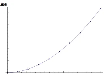
The RC collocation method is applied to solve this problem. In Table 1, the obtained numerical results are compared, for N = 12 and N = 8, with the rationalized Haar, rational Chebyshev tau method and rational Chebyshev collocation method with N = 8 and the exact solution are tabulated. The errors in numerical solution of Example 2 are shown in Fig.1. The error decreases when the integer N is increased.

Table1. Comparison between Exact solution and approximate solutions obtained by present method and other existed methods for _{y( x)}of Example 2

X Exact solution RationalizedHaar[14] RC collocation[17] RC Tau method[12] PresentMethod N=8 PresentMethod N=12

0 0 0 0 0 0 0

0.1 0.112462915907 0.11244 0.1124386 0.1124630 0.1124629 0.112462915694 0.2 0.222702588994 0.22268 0.2228901 0.2227026 0.2227025 0.222702583294 0.3 0.328626759150 0.32861 0.3285654 0.3286269 0.3286267 0.328626749513 0.4 0.428392354662 0.42837 0.4283688 0.4283925 0.4283923 0.428392342611 0.5 0.520499877374 0.52047 0.5204235 0.5204998 0.5205003 0.520499863825 0.6 0.603856090376 0.60384 0.6038157 0.6038561 0.6038590 0.603856057504 0.7 0.677801193354 0.67779 0.6776712 0.6778012 0.6778169 0.677800964362 0.8 0.742100964232 0.74208 0.7422375 0.7421011 0.7421682 0.742099890587 0.9 0.796908211971 0.79689 0.7968211 0.7969085 0.7971486 0.796905383903

Example 3

Consider the differential equation [17] ( ) ( ) ln( 1) [0,1]

1 1 ) ( ) ( ) 1 ( ′ + = + ∈ + − ′′ + ′′′

+ y x xy x x x x

1 ) 0 ( , 1 ) 0 ( , 0 ) 0

( y y

y = ′ = ′′ =−

we obtain the approximate solution by rational Chebyshev collocation function of the problem for N= 7, 12. In table 2 the numerical results obtained by the present method for N=7, 12 are compared with the R C collocation method [17] and the exact solution y(x)=ln(x+1) of this problem. Figure 2

shows the resulting graph of Example 3 for N=7 and it is compared with R C collocation method [17] and exact solution. It seen from table 2 the present method is better than R C collocation method [17]. Additionally in tables 3 and we Figure 3 compared the absolute errors for N=7 in the different methods.

Table 2. Comparison between Exact solution and approximate solutions obtained by present method and R C collocation method [17] for y(x)of Example 3

X Exact solution R C collocation method[17] N=7 Present Method N=7 Present Method N=12

0 0 0 0 0

0.1 0.09531017 0.09518485 0.09530890 0.09531019

0.2 0.18232155 0.18173604 0.18231240 0.18232170

0.3 0.26236426 0.26105289 0.26234005 0.26236469

0.4 0.33647223 0.33419588 0.33642664 0.33647311

0.5 0.40546510 0.40197707 0.40539201 0.40546660

0.6 0.47000362 0.46505273 0.46989724 0.47000589

0.7 0.53062825 0.52396995 0.53048305 0.53063142

0.8 0.58778666 0.57919041 0.58759641 0.58779089

0.9 0.64185388 0.63110549 0.64160998 0.64185930

1 0.69314718 0.68004804 0.69283674 0.69315391

Table 3. Comparison between absolute error functions obtained by present method and R C collocation method for _{y( x)}of Example 3

X e7for RCCollocation [17] e7 for presentMethod e12 for presentMethod

0 0 0 0

0.1 1.2533e-004 1.27825e-006 1.99921e-008

0.2 5.85517e-004 9.15934e-006 1.45714 e-007

0.3 1.31137e-003 2.42051e-005 4.2912 e-007

0.4 2.27636e-003 4.55917e-005 8.80284 e-007

0.5 3.48804e-003 7.31029e-005 1.49357 e-006

0.6 4.9509e-003 1.06389e-004 2.26119 e-006

0.7 6.6583e-003 1.45201e-004 3.17598 e-006

0.8 8.59625e-003 1.90248e-004 4.2315 e-006

0.9 1.07484e-002 2.43902e-004 5.42143 e-006

1 1.30991e-002 3.10434e-004 6.73649 e-006

Fig. 1. Solution graph obtained of example 2 by present method in

comparison with Other method solutions and exact solution

Fig. 2. Solution graph obtained of example 3 by present method in

Fig. 3a. Error function of Ex.3 for present method and R C collocation

method for N=7

Fig. 3b. Error function of Ex.3 for present method for N=7

Table 4. Comparison between Exact solution and approximate solutions obtained by present method for _{y( x)}of Example 4

X Exact solution Present Method N=8 Present MethodN=12 Present MethodN=16

0 1 1 1 1

0.1 0.970743243243 0.970723714463 0.970742603515 0.970743229297 0.2 0.895483870968 0.895456027695 0.895482803354 0.895483841796 0.3 0.791025179856 0.791003373112 0.791023930008 0.791025145152 0.4 0.670769230769 0.670762060806 0.670767982874 0.670769195202 0.5 0.544642857143 0.544656497125 0.544641741268 0.544642824054 0.6 0.419591836735 0.419629618122 0.419590941046 0.419591808415 0.7 0.300239726027 0.300303891194 0.300239107336 0.300239703980 0.8 0.189508196721 0.189595577331 0.189507889173 0.189508181869 0.9 0.089123616236 0.089207848147 0.089123614676 0.089123609079

1 0 0 0 0

Table 5. Comparison between absolute error functions obtained by present

method for_y(x)of Example 4 for N=8, 12 and 16

X e8 e12 e16

0 0 0 0

0.1 1.95288e-005 6.39728e-007 1.73943e-008 0.2 2.78433e-005 1.06761e-006 2.91716e-008 0.3 2.18067e-005 1.24985e-006 3.47043e-008 0.4 7.16996e-006 1.2479e-006 3.55664e-008 0.5 1.364e-005 1.11587e-006 3.30891e-008 0.6 3.77814e-005 8.95688e-007 2.83193e-008 0.7 6.41652e-005 6.18692e-007 2.20474e-008 0.8 8.73806e-005 3.07548e-007 1.48522e-008 0.9 8.42319e-005 1.56041e-009 7.15764e-009

1 0 0 0

Example 4

Consider the differential equation [16]

2

(1+ +x x )y′′′( )x + +(3 6 )x y x′′( ) 6 ( )+ y x′ =6 x x∈[0,1]

0 ) 1 ,y( 0 ) 0 ( y , 1 ) 0

y( = ′ = =

Then we have m =

3, 0 6 3 6 1 2 6 ,

3 2

1

0 ,P ,P x,P x x,g(x) x

P = = = + = + + = with exact

solution

1 x x 4 9 x 4 1 y ) x x 1

( + + 2 = 4− 2+ +

We applied the RC collocation method and solved this problem. In Table 4, 5 the resulting values for N = 8, 12 and

16 using the present method together with the exact values of

y(x)

1 4

9 4 1 ) ( ) 1

( _{+ +} 2 ₌ 4₋ 2_{+ +}

x x x x y x x

are tabulated. The error decreases when the integer N is increased.

Example 5

Consider the first order linear initial value problem ([15], P.153)

,

1

)

(

)

(

)

1

(

x

+

y

′

x

+

y

x

=

y

(

0

)

=

0

x

∈

[

0

,

1

]

Following the procedures in the previous examples, we obtain the solution of this equation in the form

T

A=_ 0 0 0_ 2

1 2 1

Therefore, we find the solution

1 ) (

+ =

x x x y

which is the exact solution of Example 5.

Example 6

Consider the fifth order linear differential equation

, ) 1 (

14 2 ) ( 180

) 1 (

5 )

5 ( 2

x x x y x

+ − =

4 1 ) 1 ( 2 1 ) 1 ( 18 ) 0 ( 5 ) 0 ( 1 ) 0

( = y′ =− y′′ = y =− y′ =−

y , , , ,

Following the procedures in the previous examples, we obtain the solution of this equation at N =8 in the form

T

A

  



−

= 0 0 0 0 0 0

2 1 2 1 0

Therefore, we find the solution

2 ) 1 (

3 1 ) (

+ − =

x x x

y

which is the exact solution of Example 6.

7. Conclusion

In this paper the use of rational Chebyshev (RC) collocation method for solving high-order linear ordinary

differential equations with variable coefficients is

investigated. The high-order linear ordinary differential equations and the given conditions to are transformed to matrix equations with unknown rational Chebyshev coefficients. This proposed technique is considered to be a modification of the similar one presented in [17]. This variant or improvement for the method gave us a faster and more accuracy much faster than the other methods. In addition, an interesting feature of this method is to find the analytical solutions if the equation has an exact solution that is a rational functions. Illustrative examples are used to demonstrate the applicability and the effectiveness of the proposed technique. The method can be extended for the case of systems of linear differential equations with variable coefficients which is under investigation by the authors.

References

[1] G. Yuksel, M. Gulsu and M. Sezer,” A Chebyshev Polynomial Approach for Higher – Order Linear Fredholm- Volterra Integro-Differential Equations, Gazi University Journal of Science,25(2), 393 – 401 , 2012.

[2] S. Abbasbandy, H. Ghehsareh and I. Hashim, “An approximate solution of the MHD flow over a non-linear stretching sheet by rational Chebyshev collocation method “, U.P.B. Series A, Vol.74, Issue. 4, 2012.

[3] K. Parand and M. Razzaghi, Rational Chebyshev tau method for solving Volterra population model, Applied Mathematics and Computation 149 (2004) 893–900.

[4] D. Funaro and O. Kavian, Approximation of some diffusion evolution equations in unbounded domains by Hermite function, Math. Comp. 57, 597-619, 1990.

[5] B.Y. Guo, Error estimation of Hermite spectral method for nonlinear partial differential equation, Math. Comp. 68, 1067-1078, 1999.

[6] B.Y. Guo and J. Shen, Laguerre-Galerkin method for nonlinear partial differential equations on a semi-infinite interval, Numer. Math. 86, 635-654, 2000.

[7] J. Shen, Stable and efficient spectral methods in unbounded domains using Laguerre functions, SIAM J. Numer. Anal. 38, 1113-1133, 2000.

[8] B.Y. Guo, Jacobi spectral approximation and its applications to differential equations on half line, J. Comput. Math. 18, 95-112, 2000.

[9] J.P. Boyd, Orthogonal rational functions on a semi-infinite interval, J. Comput. Phys. 70, 63-88, 1987.

[10] J.P. Boyd, Spectral methods using rational basis functions on an infinite interval, J. Comput. Phys. 69, 112-142, 1987. [11] H.I. Siyyam, Laguerre tau methods for solving higher-order

ordinary differential equations, J. Comput. Anal. Appl. 3, 173-182, 2001.

[12] K. Parand and M. Razzaghi, Rational Chebyshev tau method for solving higher- order ordinary differential equations, Inter. J. Comput. Math. 81, 73-80, 2004.

[13] M. Sezer and M. Kaynak, Chebyshev polynomial solutions of linear differential equations, Int. J. Math. Educ. Sci. Technol. 27(4), 607-618, 1996.

[14] Salih Yalçınbaş, Nesrin Özsoy and Mehmet Sezer, Approximate solution of higher order linear differential equations by means of a new rational Chebyshev collocation method, Mathematical and Computational Applications, Vol. 15, No. 1, pp. 45-56, 2010.

[15] L. Fox and I.B. Parker, Chebyshev polynomials in Numerical Analysis, Oxford University press, Ely House, London, 1968. [16] Daniel Zwillinger, Handbook of Di®erential Equations,

Academic Press, Boston, 1997.