Algorithms for Sparse Linear Classifiers in the Massive Data Setting

Algorithms for Sparse Linear Classifiers in the Massive Data Setting

Suhrid Balakrishnan [email protected]

Department of Computer Science Rutgers University

Piscataway, NJ 08854, USA

David Madigan [email protected]

Department of Statistics Columbia University New York, NY 10027, USA

Editor: Peter Bartlett

Abstract

Classifiers favoring sparse solutions, such as support vector machines, relevance vector machines, LASSO-regression based classifiers, etc., provide competitive methods for classification problems in high dimensions. However, current algorithms for training sparse classifiers typically scale quite unfavorably with respect to the number of training examples. This paper proposes online and multi-pass algorithms for training sparse linear classifiers for high dimensional data. These algorithms have computational complexity and memory requirements that make learning on massive data sets feasible. The central idea that makes this possible is a straightforward quadratic approximation to the likelihood function.

Keywords: Laplace approximation, expectation propagation, LASSO

1. Introduction

We consider the problem of learning high-dimensional sparse linear classifiers from large numbers of training examples. A number of different applications from finance, text mining, and bioinfor-matics motivate this work. We concern ourselves specifically with binary classification and consider

L1-regularized logistic and probit regression models. Such models have provided excellent

predic-tive accuracy in many applications (see, for example, Genkin et al., 2007; Figueiredo and Jain, 2001; Shevade and Keerthi, 2003) and attack overfitting and variable selection in a unified manner.

L1-regularization and a maximum a posteriori (MAP) Bayesian analysis with so-called Laplacian

priors yield identical results (Tibshirani, 1996) and in order to streamline our presentation, we adopt

the Bayesian approach. Many training algorithms now exist for L1-logistic regression that can

han-dle high-dimensional input vectors (Hastie et al., 2004; Shevade and Keerthi, 2003; Koh et al., 2007). However, these algorithms generally begin with a “load data into memory” step that pre-cludes applications with large numbers of training examples. More precisely, consider a training

data set that comprises t examples each of dimension d. Due to matrix multiplications on t_×t or

d_×d matrices, typical computational time requirements are O(t3_+d3_{), with memory requirements}

that are O(td+d2). In our target applications, both t and d can exceed 106so standard algorithms

This paper presents two basic algorithms for learning L1-logistic and/or probit regression

mod-els. Both operate in the data streaming model, by which we mean that they scan the data sequen-tially, and never require storing processed observations. The first algorithm we present is an online algorithm which sequentially processes each observation only once. This algorithm is provably

non-divergent and uses in the worst case O(d2)time and O(d2) space to assimilate each new training

example (note that both costs are constant with respect to the number of observations, t). Further, if the input data are sparse, the practical computational cost can be significantly lower.

For massive data sets where t is constant, that is, when given a fixed training data set, we present a second algorithm that allows practitioners to trade-off computational time for improved accuracy. This multi-pass algorithm (the MP algorithm) also processes data sequentially but makes a small constant number of extra passes over the data set. Hence, this sequential algorithm provides results similar to those of batch algorithms for this problem. The MP algorithm’s computational cost is a constant factor higher and memory costs are essentially the same as those of the online algorithm. Finally, we propose the RMMP (Reduced Memory MP) algorithm that has significantly lower worst

case memory costs, O(d+k2)(where kd) and the same computational costs as the MP algorithm

(thus both computational and memory costs are essentially linear in t and d). We will comment on the similarities and differences of our technique to other learning algorithms, in particular other online algorithms, in the following sections.

2. Background and Notation

Throughout this manuscript, we concern ourselves with the task of binary classification, with class labels y_{∈ {}0,1_}. The training data comprise t labeled training examples, that is, Dt={(xi,yi)}ti=1,

with input vectors xi = [xi1, . . . ,xid]T inRd and corresponding labels yi, i=1, . . . ,t. We consider

probabilistic classifiers of the form:

p(y=1_|x) =Φ(βTx)

where β_∈Rd is a vector of regression parameters and Φ(_·) is a link function. We restrict our

analytical results to the two most commonly used link functions, the probitΦ(z) =Rz

−∞√12πe −x2_/2

dx

and logisticΦ(z) = ez

1+ez link functions.

The machine learning problem is thus to estimate the parameters β, in the light of the training

data Dt. We tailor our results towards high input dimension, that is, large d, and large numbers of

training vectors, large t. Viewing the learning problem as one of Bayesian inference, we work with

the posterior distribution of the parametersβconditioned on a labeled training data set Dt, given a

prior distribution on the parametersβ:

p(β_|Dt)∝ t

∏

p(yi|β) !

p(β). (1)

The quantity on the left hand side of (1) is the required posterior distribution ofβgiven the data set

Dt, while the second term on the right hand side is the prior distribution onβ, which we will specify

momentarily. The first term on the right hand side is the likelihood:

t

∏

p(yi|β) = t

∏

yiΦ(βTxi) + (1−yi)(1−Φ(βTxi)

Finding the MAPβleads to the optimization problem we wish to solve (now on the log scale):

max

β (log p(β|Dt))

≡ max

β t

∑

logyiΦ(βTxi) + (1−yi)(1−Φ(βTxi)

−log p(β) !

. (2)

The prior distribution p(β)we pick for the parameters is the LASSO prior (Tibshirani, 1996), a

product of independent Laplacian or double-exponential prior distributions on each componentβj

(with mean 0):

p(βj|γ) = γ 2e

−γ|βj|_,γ_{>0,j=1, . . . ,d.}

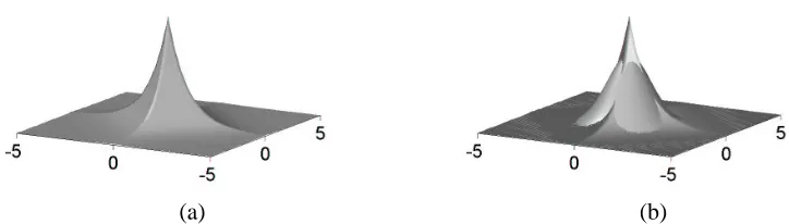
A prior of this form places high probability mass near zero and along individual component axes. It also has heavier tails than a Gaussian distribution—see Figure 1 for plots of the 2-dimensional distributions. It thus favors locations in parameter space with component magnitudes either exactly

(a) (b)

Figure 1: (a) A standard Laplacian distribution,γ=1 (b) A superposition of standard (zero mean,

unit variance) Gaussian distribution, and the Laplacian distribution showing both the higher probability mass the Laplacian assigns along the axes and at zero as well as its heavier tails.

zero, and hence pruned from our predictive model, or shrunk towards zero. With this prior distri-bution, (2) presents a convex optimization problem and yields the same solutions as the LASSO (Tibshirani, 1996) and Basis Pursuit (Chen et al., 1999):

max

β (log p(β|Dt))

≡ max

β t

∑

log

yiΦ(βTxi) + (1−yi)(1−Φ(βTxi)

−γkβk1 !

. (3)

The parameter γin the above problem controls the amount of regularization. Figure 2 shows

asγis varied. The choice of the regularization parameter is an important but separate question in itself (Efron et al., 2004; Hastie et al., 2004). Methods such as cross validation can be used to pick its value and algorithms also exist to find solutions for all values of the regularization parameter (commonly called regularization path algorithms). However, we do not address such issues in this

manuscript, and we simply assumeγis some fixed, user-specified constant.

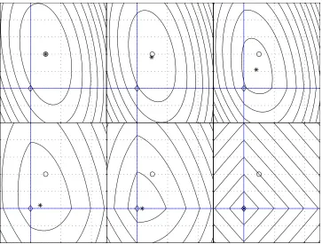
Figure 2: L1-regularization in two dimensions (i.e., d=2). The axes are the solid lines, the

horizon-tal axis representingβ1and the vertical axis representingβ2. The diamond represents the

origin and the open circle represents the (non-regularized) maximum likelihood solution. The figure shows contours of the function in (3), the objective function, for increasing amounts of regularization (right to left and then top to bottom). The star shows the MAP location. The top row, left figure, shows negligible regularization; the MAP and

maxi-mum likelihood estimates coincide and the contours show no L1-induced discontinuities.

The top row, right figure, shows noticeable L1effects and the MAP and maximum

likeli-hood solutions differ. The bottom row, middle panel shows enough L1-regularization to

setβ2 to zero (i.e., variable selection has occurred). The bottom row, right panel, shows

extreme regularization, where bothβ1andβ2are zero.

To the best of our knowledge, all existing algorithms solve the above convex optimization

prob-lem in the batch setting, that is, by storing the data set Dt in memory and iterating over it (Fu, 1998;

now attempts to overcome this limitation and thereby provide algorithms for training sparse linear classifiers without loading the entire data set into memory.

3. Approximating the Likelihood for Online Learning

The Bayesian paradigm supports online learning in a natural fashion; starting from the prior, the first training example produces a posterior distribution incorporating the evidence from the first example. This then becomes the prior distribution awaiting the arrival of the second example, and so on. In practice, however, except in those cases where the posterior distribution has the same mathematical form as the prior distribution, some form of approximation is required to carry out the sequential updating.

We want to avoid algorithms that begin with a “load data into memory” step and also avoid memory costs that increase with increasing amounts of data. In other words, we want memory costs independent of t. This requirement in turn, necessitates that we “forget” examples after processing

them. We achieve this by maintaining the sufficient statistics of a quadratic approximation inβto

the log-likelihood of the parameters after incorporating each observation. We approximate the log-likelihood as:

t

∑

log(p(yi|β)) = t

∑

log

yiΦ(βTxi) + (1−yi)(1−Φ(βTxi)

≈

t

∑

ai(βTxi)2+bi(βTxi) +ci

,

where ai(βTxi)2+bi(βTxi) +ci approximates logΦ(βTxi)when yi=1 and approximates log(1− Φ(βTxi))when yi=0, i=1, . . . ,t. In either case the approximation uses a simple Taylor

expan-sion around βT_i−1xi, where βi−1 estimates the posterior mode given the first i−1 examples, Di−1

(Appendix A provides expressions for ai,bi for the probit and logistic link functions). We then

have:

t

∑

log(p(yi|β)) ≈ t

∑

ai(βTxi)2+bi(βTxi) +ci

= t

∑

ai(βTxi)(xTi β) + t

∑

bi(βTxi) + t

∑

ci

= βTΨtβ+βTθt+ t

∑

ci

where:

Ψt= t

∑

aixixTi, andθt= t

∑

bixi.

We now substitute this approximation of the log-likelihood function into Equation (3) to obtain the modified (approximate) optimization problem:

max

β (log p(β|Dt))≈maxβ

βT_Ψ

tβ+βTθt−γkβk1

Note that we can ignore the term involving the ci’s, as it is not a function ofβ. Further, the fixed

size d_×d matrixΨand the d_×1 vectorθcan be updated in an online fashion as data accumulate:

Ψt+1=Ψt+at+1xt+1xTt+1, andθt+1=θt+bt+1xt+1. (5) The size of the optimization problem in (4) doesn’t depend on t, the size of the data set seen so far. Thus, solving a fixed (with respect to t) size optimization problem allows one to sequentially process labeled data items and march through the data set. In data streaming terminology, the matrix

Ψand the vectorθprovide a constant size sketch or summary of the labeled observations seen so

far.

A number of questions now present themselves: how good is this approximation? How do we solve the approximate optimization problem efficiently? How does this approach differ from other likelihood approximation schemes (some of which are also quadratic)? Also, the scheme as set

up requires O(d2) memory in the worst case. Since we would like to use this approach for high

dimensional data sets, can we reduce the memory requirements?

The remainder of this manuscript addresses these and other questions. First, we consider how to efficiently obtain the MAP solution of (4), the approximate optimization problem.

3.1 The Modified Shooting Algorithm

Recall that we need to findβthat solves:

max β

βT_Ψβ+βT_θ

−γkβk1

. (6)

In the above equation and following discussion, we drop the subscript t from Ψ,θfor notational

convenience. This is a convex optimization problem and a number of efficient techniques exist to solve it. Newton’s method and other Hessian-based algorithms may be prohibitively expensive

as they need O(d3) computational time in order to construct the Hessian/invert d_×d matrices.

Other authors have described good results on the arguably tougher (non-approximate) optimization

problem for logistic regression (essentially the terms in Equation 3, but with L2regularization ofβ)

with techniques such as fixed memory BFGS (Minka, 2000), modified conjugate gradient (Komarek and Moore, 2005) and cyclic coordinate descent (Zhang and Oles, 2001; Genkin et al., 2007).

In this paper, we employ instead a slight modification of the Shooting algorithm (Fu, 1998), see Algorithm 1. Shooting is essentially a coordinate-wise gradient ascent algorithm, explicitly tailored

for convex L1-constrained regression problems (squared loss). Since our approximate optimization

problem is also quadratic, the resulting modifications required are straightforward. The vector Ω

in the algorithm is defined asΩ=2Ψ0β+θ, whereΨ0is the matrixΨwith its diagonal entries set

to zero (see Appendix B for details). This vector is related to the gradient of the differentiable part of the objective function and consequently can be used for optimality checking. Minor variants of this algorithm have been independently proposed by Shevade and Keerthi (2003) and Krishnapuram et al. (2005). Although Fu originally derived the algorithm by taking the limit of a modified Newton-Raphson method, it can also be obtained by a subgradient analysis of the system (subgradients are

necessary due to the non-differentiability that the L1constraints onβresult in, see Appendix B for

the derivation).

While one can think of numerous stopping criteria for the algorithm, in this paper we stop

Algorithm 1: The modified Shooting algorithm. Data: Ψ,θ,β₀,γ.

β₀is initialβvector.

Ωjrefers to the j’th component ofΩ.

Ψj jrefers to the(j,j)’th element of matrixΨ. Result: βsatisfying (6).

while not converged do for j_←1 to d do

βj=   

 

0, if_|Ωj| ≤γ

γ−Ωj

2Ψj j, ifΩj>γ −γ−Ωj

2Ψj j , ifΩj<−γ

UpdateΩ.

end end

norm). More precisely, we declare convergence whenever_kβ_i−β_i−1k2/kβi₋1k2is less than some

user specified tolerance. Note thatβ_i is the parameter vector at iteration i, which is obtained after

cycling through and updating all d components once.

In the worst case, each iteration of Shooting requires O(d2)computational time. However, for

reasonable amounts of regularization, where the final set of non-zero βvalues is small, the time

requirements are much smaller. Indeed, the practical computational cost is perhaps better reflected

by bounds in terms of the sparsity of MAP β. Let m denote the maximum number of non-zero

components ofβalong the solution path to MAPβ(hence m≤d). Implemented carefully, Shooting

requires O(md) time per iteration (see Appendix B for details). Shooting can be initialized with

β₀=0 if no information about the optimalβis known or to an appropriate “warm” starting point.

While coordinate-wise approaches are commonly regarded as slow in the literature (for example, Minka, 2001a), for sparse classifiers, they are much faster (see for example, Shevade and Keerthi, 2003). In our experiments, the Shooting algorithm has proven to be practical even for d in the hundreds of thousands.

4. An Online Algorithm

The quadratic approximation and the Shooting algorithm lead straightforwardly to an online

algo-rithm. After initializing the sketch parameters Ψ0,θ0 and the initial parameter vectorβ0, process

the data set one observation at a time. Calculate the quadratic Taylor series approximation to each

observation’s log-likelihood at the current estimate of the posterior mode,β_i−1, thus finding

param-eters ai,bi. Use these parameters and the observation to update the sketches, Ψ,θ. Now run the

modified Shooting algorithm to update the posterior mode, producing β_i and repeat for the next

labelled observation—see Algorithm 2.

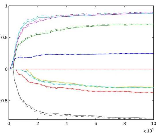
We show the performance of the online algorithm on a low dimensional simulated data set

in Figure 3 (the data generating mechanism is a logistic regression model with d=11, and t =

100,000. For details see the Experiments section of the manuscript). As we process greater

Algorithm 2: The Online algorithm. Data: Dt,γ.

Result: For each i, producesβ_i, an approximation to the MAP estimate ofβfor observations

(x1,y1). . .(xi,yi).

Initializeβ₀=θ0=0,Ψ0=0, i=1. while i<t do

Get i’th observation(xi,yi).

Obtain quadratic approximation to term likelihood atβ_i−1, that is, obtain ai,bi. Ψi←Ψi−1+aixixTi .

θi←θi−1+bixi.

β_i←modified Shooting(Ψi,θi,βi−1,γ)

i_←i+1.

end

estimates (the dashed lines which we obtain using BBR, Genkin et al. 2007, publicly available

software for batch L1penalized logistic regression). See Figure 3, where different colors represent

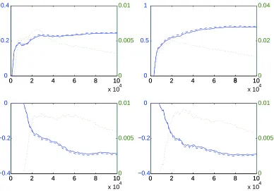
different components of MAPβ_i. Figure 4 shows individual plots of the online and batch estimates

for four representative components of MAPβ_iin blue. We also plot the absolute difference between

the batch and online estimates in green (dotted line) on the same plot on the right (green) axis. As we expect, after the parameter estimates stabilize, this difference steadily tapers off with increasing amounts of data.

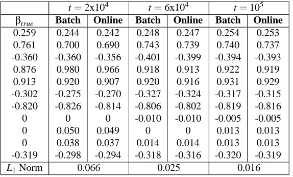
t=2x104 t=6x104 t=105

βtrue Batch Online Batch Online Batch Online

0.259 0.244 0.242 0.248 0.247 0.254 0.253 0.761 0.700 0.690 0.743 0.739 0.740 0.737 -0.360 -0.360 -0.356 -0.401 -0.399 -0.394 -0.393 0.876 0.980 0.966 0.918 0.913 0.922 0.919 0.913 0.920 0.907 0.920 0.916 0.931 0.929 -0.302 -0.275 -0.270 -0.327 -0.324 -0.317 -0.315 -0.820 -0.826 -0.814 -0.806 -0.802 -0.819 -0.816

0 0 0 -0.010 -0.010 -0.005 -0.005

0 0.050 0.049 0 0 0.013 0.013

0 0.038 0.037 0.014 0.014 0.013 0.013 -0.319 -0.298 -0.294 -0.318 -0.316 -0.320 -0.319

L1Norm 0.066 0.025 0.016

Table 1: Table with columns showing values ofβ_true, and the MAP estimates ofβobtained by the

batch algorithm and the online algorithm, for increasing amounts of data on the simulated data set. To aid assessing convergence of the online to the batch estimates, we show the

value of the L1norm of the adjacent vectors (batch vs. online estimates) in the last row.

For this example,γ=10 (logistic link function).

In the worst case, the online algorithm requires O(d2)space and O(d2)computational time to

0 2 4 6 8 10 x 104 1

0 0.5

−0.5

Figure 3: Performance of the online algorithm on a simulated data set, with regularization

parame-terγ=100 (see text for details). The y-axis is the parameter value, the x-axis the number

of observations processed, t.

which is true of text data for instance, the algorithm leverages this. Let the maximum number of non-zero components in any x be f and assume a constant number of iterations of the modified Shooting algorithm. In such case, the practical computational time requirement of the algorithm is

O(f2+md)per observation (we remind the reader that the md term, is for the cost of the Shooting

algorithm—see 3.1). Although the practical memory costs of the algorithm will likely be less than

O(d2), exactly how much less depends heavily on the data, since Ψ(the part of the sketch

domi-nating the memory requirements) is a weighted sum of outer products of the xi’s. It is possible that

even very sparse data may result in the full O(d2)memory requirement.

Here, we highlight the fact that the online algorithm is accurate and practical if the problem is of low to medium input dimension, but massive in terms of the number of observations. Appendix C proves non-divergence of the algorithm in the infinite data limit.

4.1 Heuristics for Improvement/Issues

While one can also obtain parameter estimates for fixed t ( batch problems) using the online algo-rithm, multiple passes typically provide better estimates, albeit with increased computational cost.

Denote byβ_∗the solution to the exact optimization problem (3) for some fixed t. Since the online

algorithm typically initializes itself far fromβ_∗, it is only after processing a sufficient number of

examples that the online algorithm’s term approximations will start being taken closer toβ_∗. The

0 2 4 6 8 10 x 104

0 0.2 0.4

0 2 4 6 8 100

0.005 0.01

0 2 4 6 8 10

x 104

0 0.5

1

0 2 4 6 8 100

0.02 0.04

0 2 4 6 8 10

x 104

−0.4 −0.2 0

0 2 4 6 8 100

0.005 0.01

0 2 4 6 8 10

x 104

−0.4 −0.2 0

0 2 4 6 8 100

0.005 0.01

Figure 4: Slightly more detailed version of Figure 3. The panels show four representative

parame-ters from that figure, also showing tapering L1loss (dotted green line) between the online

and batch algorithm estimates on the right axis (in green). Simulated data set,γ=100.

Once again, the (left) y-axis is the parameter value and the x-axis the number of observa-tions processed, t.

magnitude than their respective final values,Ψt,θt. However, the amount of regularization remains

relatively fixed atγkβk1. Hence, if the online algorithm is initialized atβ0=0, for any i<t, the

output MAP estimateβ_i will be more shrunk towards zero thanβ_∗. Figure 3 illustrates this for

smaller values of t where the solid lines (approximate MAP estimates) are closer to zero than the dashed lines (exact batch estimates).

This suggests the following two heuristics to improve the quality of estimates from the online algorithm. The first is to increase the amount of regularization gradually as the algorithm processes

observations sequentially (via a schedule, linearly say,∝t from zero initially to the specified value

γat the end of the data set1). Less regularization of the first few observations somewhat mitigates

the effect of taking term approximations at shrunken parameter estimates.

The second heuristic is for the online algorithm to keep a block of observations in memory temporarily instead of immediately discarding each observation after processing it. The algorithm

then uses the value of the parameter estimates after having seen/processed all the observations in a block to update the sketches for the whole block. Note that this will involve keeping track of

the corresponding updates to the sketches for the block (the block’s contributions toΨandθ). In

experiments not reported here, both of these heuristics improve the final online estimates somewhat.

One possibility for improving upon the O(d2) worst case computational requirement of the

online algorithm is as follows. In the infinite data case, in order to obtain sparsity in parameter estimates, the amount of regularization must be allowed to increase as observations accumulate— an increasingly weighty likelihood term will inundate any fixed amount of regularization. In this setting (where we have the freedom to choose the amount of regularization), we can use exactly

the same quadratic approximation machinery to pick the value ofγthat maximizes the approximate

one-step look ahead likelihood (although the expressions for this approximation would be slightly different). The resulting scheme has the flavor of predictive automatic relevance determination as presented in Qi et al. (2004).

The worst case O(d2)memory requirement of the online algorithm, however, presents a greater

challenge. In the next section we outline a multi-pass algorithm based on the same sequential quadratic approximation that improves the accuracy of estimates when applied to finite data sets and also uses less memory than the online algorithm.

5. A Multi-pass Algorithm

The block heuristic of the previous section implies that taking all term approximations at the final

online algorithm MAP β_t value would certainly produce better estimates of Ψt,θt. This in turn

would lead to a better estimate ofβ_∗.

Therefore, for fixed data sets where computational time restrictions still permit a few passes over the data set, this suggests the following algorithm, which we will refer to as the MP

(Multi-Pass) algorithm: Initializeβ₀=θ0=0, Ψ0=0, z=1. The quantity z will count the number of

passes through the data set. ComputeΨt,θt by the steps in Online Algorithm (Algorithm 2), except

take all term approximations at the fixed valueβ_z. Note that consequently there is no need for the

shooting algorithm during the pass through the data set. Once a pass through the data set is

com-plete, compute a revised estimate ofβ_∗ by running modified Shooting, that is, setβ_z+1=modified

Shooting(Ψt,θt,βz,γ). Iteratively loop over the data set, appropriately incrementing z.

For a constant number of passes, the MP algorithm has the worst case computational time

re-quirement of O(td2) to do an equivalent batch MAP β estimation. Once again, if the data set

is sparse, this cost is closer in practice to O(t f2+md) (the first term is the cost of updating the sketches and the second md term is the cost of the Shooting algorithm).

The worst case memory requirement of the MP algorithm is O(d2), which is just a constant with

respect to t. Expectation Propagation (Minka, 2001b) by contrast requires explicitly storing term

ap-proximations and thus has memory costs that scale linearly with t, that is, O(t). The next subsection

presents a modification of the MP algorithm that reduces this worst case memory requirement.

5.1 A Reduced Memory Multi-pass Algorithm

The key to reducing the memory requirements of the algorithm in the previous subsection is

ex-ploiting the sparsity ofβ_∗. Towards this end, consider the modified Shooting algorithm upon

con-vergence; sayβ_MAPis the sparse converged solution Shooting obtains with inputsΨ,θandγ. Now

corre-sponding columns for matrices, for which the components ofβ_MAPare nonzero (denoted with a ˜). The important observation is that the solution to the reduced size system ˜β_MAP, obtained using ˜Ψ,θ˜

and ˜Ω, has exactly the same nonzero components asβ_MAPobtained for the full system.

We use this fact to derive the RMMP (Reduced Memory Multi-Pass) algorithm, Algorithm 3. The central idea is to use the optimality criteria for the Shooting algorithm to determine which

components ofβto keep track of. Call this set S, the active set, which is fixed during every iteration.

Specifically, we set S=_{j :_|Ωj| ≥γ}. That is, the active set is the set of variables that are either

nonzero and optimal or variables that violate optimality at the start of a pass (the corresponding nonzero elements of the vectors/matrices are denoted by their previous symbols but with a ˜ above

them). Now, during the pass we keep track of the much smaller matrix ˜Ψ, while also keeping

track of the unmodified/original full length vectorsθandΩ. The update forθis unchanged and

Appendix B shows how to perform the update for the full length vectorΩ in small space. The

algorithm continues by using ˜Ψ,Ω, andθfrom the latest pass to re-estimate the active set, S and so

on.

A desirable consequence of the setup is that no new approximation is introduced. The search for the optimal parameter values is slightly more involved though, now proceeding iteratively by

first identifying candidate nonzero components ofβ_MAP, and then refining the estimates for these

components. We can employ the same stopping criteria as for modified Shooting algorithm.

Algorithm 3: The RMMP algorithm. Data: fixed data set Dt,γ.

Result: β_z, the MAP estimate ofβthat solves (3). Initializeβ₀=0, S=_{},z=1.

while not converged do

Setθ=0, ˜Ψ=0, i=1.

for i=1,2, . . . ,t do

Get i’th observation(xi,yi).

Obtain quadratic approximation to term likelihood atβ_z−1, that is, obtain ai,bi.

˜

Ψ←_Ψ˜ _+ai(x˜ix˜iT_). θ_←θ+bixi.

UpdateΩ.

end

βz←modified Shooting( ˜Ψ,θ˜,β˜z₋1,γ).

Obtain new active set S=_{j :_|Ωj| ≥γ}. z_←z+1.

end

Note that memory requirements are now O(d+k2), where k is the number of variables in the

largest active set. However, we can be even more stringent and set k to be a user specified constant

provided k is bigger than the final number of nonzero components ofβ_∗. Typically, setting k very

close to this limit results in some loss of accuracy and the cost of a few more passes over the data for convergence. The worst case computational time requirements for a constant number of passes,

are still O(td2_{)to do an equivalent batch MAP}β_{estimation. Under the same sparsity assumptions}

We now draw attention to a few practical considerations about the RMMP algorithm. The first

is that although we consider initializing the parameter vector to zero, β₀=0, better guesses of

β₀ (guesses closer to the MAP β) would likely result in fewer passes for convergence. Further,

given we do initialize at zero, the first pass is completed very rapidly. This is because no outer products are computed, since the active set is initialized as the empty set; the first pass is used simply to determine the size and components of the active set and the parameter estimates for the

next iteration are still zero,β₁=0. Typically, setting the reduced memory parameter k to be larger

than this first active set size results in further RMMP iterations mimicking iterations of the MP algorithm. This is seen by observing two facts. One, for both algorithms, the only components that change in successive iterations are those in the active set (components that are either non-zero and

optimal or not optimal). Two, in a typical search path for the MAP β, the size of the active set

decreases (and finally stabilizes) as the MAPβis honed in on. Both of these observations together

imply that if we start the RMMP algorithm with enough memory allotted to look at all possibly

relevantβcomponents, we will follow the MP search path (as a motivating example, consider that

setting k=d results in the MP algorithm exactly).

Another consideration is a very useful practical advantage of the proposed algorithm:

knowl-edge ofΩimplies the practitioner can confirm when convergence to β_∗ has/has not occurred. In

practice, for numerical stability, slightly expanding the active set seems to be a good heuristic. In our experiments that follow, we do so only if we have extra space (if k is bigger than the number of variables in the current active set, for any iteration) in two ways: 1. We retain in the active set vari-ables that were in the active set in the previous iteration and, 2. we add to the active set components that are close to violating optimality (close in terms of a threshold,τ<1. This amounts to replacing the rule in Algorithm 3 with S=_{j :_|Ωj| ≥τγ}).

In the next section, we place our work in the context of existing literature on similar problems.

6. Related Work

Although the Bayesian paradigm facilitates sequential updating of the posterior distribution (online learning) in a natural way, some form of approximation is almost always necessary for practical applications. Approximating the posterior distribution at every stage by a multivariate Gaussian distribution (which implies a quadratic approximation of the log posterior distribution) seems a natural first step backed by asymptotic Bayesian central limit results that imply this approximation will get better and better with the addition of data (Bernardo and Smith, 1994).

Indeed, approximating the log-likelihood function by a quadratic polynomial is a standard technique in Bayesian learning applications; see for example Laplace approximation (Kass and Raftery, 1995; MacKay, 1995), Assumed Density Filtering (ADF)/Expectation Propagation (EP) (Minka, 2001b), some variational approximation methods such as Jaakkola and Jordan (2000) and in Bayesian online learning (Opper, 1998). We would like to stress here that many of the above schemes are for the harder task of approximate inference—we are concerned only with the easier problem of approximate convex optimization. The similarities in the approaches are confined to the nature of the approximate (Gaussian) posterior.

7. Experiments

We now present examples illustrating the application of the Online, MP and RMMP algorithms to simulated data sets, where we control the data generating mechanism, and some real data sets. We make logistic regression comparisons to results obtained using BBR (Genkin et al., 2007). BBR is publicly available software for Bayesian binary logistic regression that handles the Laplacian prior. We make probit regression comparisons to results obtained using a batch EM algorithm for Lapla-cian prior based probit regression (we implemented a slightly modified version of the algorithm in Figueiredo and Jain, 2001). We generally do not present prediction accuracy results here as our goal is to obtain accurate, that is, close to batch, parameter values. What we wish to accomplish with the experiments is demonstrate practical efficiency and applicability of the algorithms. In so doing and by obtaining essentially identical parameter estimates to batch algorithms, our predictive per-formance will mirror those of the batch algorithms. Several papers provide representative predictive

performance results for L1-regularized classifiers, for example, Genkin et al. (2007); Figueiredo and

Jain (2001).

We carried out all the experiments on a standard Windows OS based 2Ghz processor machine with 1GB RAM. For all experiments we set the modified Shooting convergence tolerance to be

10−6, andτ=0.8 (for experiments involving the RMMP algorithm).

We use the following data sets:

• Simulated data sets: d=11, t=10,000. The data generating mechanism is either a probit or

lo-gistic regression model with one intercept term and 10 model coefficients, for a total of 11 fixed parameters. Of the ten model variables, three are intentionally set as redundant variables (set with zero coefficients in the model). The data vectors x, are draws from i.i.d. Gaussian distributions with mean zero and unit variance. For the experiments with the online algorithm (Figure 3, Table 1),

we used the same model parameters as above, but with t=100,000 and only a logistic regression

model.

• ModApte training data set: d=21,989, t=9,603. This is a text data set, the ModApte split of

Reuters-21578 (Lewis, 2004). We examine one particular category, “earn”, to which we fit a logistic regression model.

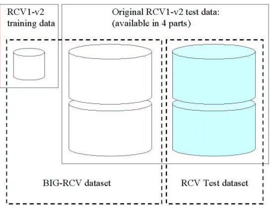
• BIG-RCV data set: d=288,062, t=421,816, a data set constructed from the RCV1-v2 data set

(Lewis et al., 2004). It consists of the training portion of the LYRL2004 split plus 2 parts of the test

data (the test data is made publicly available in 4_≈350 MB parts)—see Figure 5. We also use just

the training portion of RCV1-v2 in some experiments. RCV1-v2 training data set : d=47,236,

t=23,149 (the features in this data set are a particular subset of the features in BIG-RCV). Our

results are for a single topic “ECAT”, whether or not a document is related to economics.

7.1 Results

The low dimensional simulated data set highlights typical results we obtain with the Online algo-rithm and the MP algoalgo-rithm (the RMMP algoalgo-rithm is not of practical significance in this case). See

Table 2. Each column in the table is an 11-dimensional vector which is the MAPβestimate of the

Figure 5: Schematic showing the construction of the various RCV1-v2 based data sets used in the experiments. The solid line bordered rectangles show the data as publicly available, the dashed-line bordered rectangles show the data sets we assembled. The shaded portion of the data is used only during testing.

functions and over a wide range of settings for the regularization parameter,γ. To show this, the

tables report results for both too little regularization (γ=10, probit link) and too much

regulariza-tion (γ=100, logistic link) for this particular data set. As a guide to assessing convergence in this

and other tables that follow, we show the L1 norm of the difference between the batch algorithm

estimates (EM or BBR as appropriate) and the Online, MP or RMMP algorithm iterates (also as appropriate).

We next examine the first real data set, the training data for the ModApte split of

Reuters-21578 (Lewis et al., 2004). This is a moderate dimensional (d =21989 features) data set with

t=9603 labelled observations (we use the feature vectors that can be downloaded from the paper’s

appendix.). The features of this data set are weighted term occurrences and it is quite sparse, as is typical for text data. The batch EM algorithm for probit regression is prohibitively expensive on this data set as it involves inverting a high dimensional matrix, but we can run BBR to obtain batch logistic regression results. Hence we focus our results on logistic regression for this data set. We

examine two reasonable settings for the regularization parameter,γ=10 andγ=100. Forγ=10,

BBR returns 150 nonzero components and forγ=100, the MAPβBBR returns has 31 non-zero

components. Since the data set is sparse, and presents no memory limitations, we are able to apply the Online and MP algorithms in addition to the RMMP algorithm—see Tables 3 and 4.

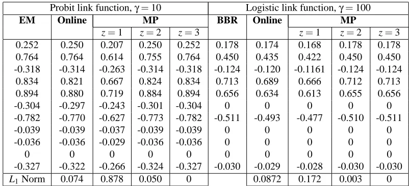
Probit link function,γ=10 Logistic link function,γ=100

EM Online MP BBR Online MP

z=1 z=2 z=3 z=1 z=2 z=3 0.252 0.250 0.207 0.250 0.252 0.178 0.174 0.168 0.178 0.178 0.764 0.764 0.614 0.755 0.764 0.450 0.435 0.422 0.450 0.450 -0.318 -0.314 -0.263 -0.314 -0.318 -0.124 -0.120 -0.1161 -0.124 -0.124 0.834 0.821 0.667 0.824 0.834 0.713 0.689 0.666 0.712 0.713 0.894 0.880 0.719 0.884 0.894 0.656 0.634 0.613 0.655 0.656

-0.304 -0.297 -0.243 -0.301 -0.304 0 0 0 0 0

-0.782 -0.770 -0.627 -0.773 -0.782 -0.511 -0.493 -0.477 -0.510 -0.511

-0.039 -0.039 -0.037 -0.039 -0.039 0 0 0 0 0

-0.036 -0.036 -0.029 -0.036 -0.036 0 0 0 0 0

0 0 0 0 0 0 0 0 0 0

-0.327 -0.322 -0.266 -0.324 -0.327 -0.030 -0.029 -0.028 -0.030 -0.030

L1Norm 0.074 0.878 0.050 0 0.0872 0.172 0.003 0

Table 2: Table with columns showing values of the MAP estimates of β obtained by the batch

algorithms (EM on the left half, for probit regression and BBR on the right half for logistic regression), the Online algorithm and three successive iterates of the MP algorithm applied

to the simulated data set. The final row displays the L1 norm of the difference between

the batch algorithm estimates (EM or BBR as appropriate) and the Online/MP algorithm estimates. The results shown here are representative of those obtained for other values of γas well.

as expected. Forγ=100, the MP algorithm converges in about z=6 iterations to parameter values

indistinguishable from BBR—see the left three columns in Table 3. We next applied the RMMP

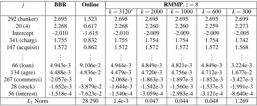
algorithm to this data set. Examining the size of the first active set reveals setting k_≈3000, would

give exactly the same results as the MP algorithm—see typical effects of changing k in Table 4 for

γ=10. We point out that this is a huge reduction in the worst case memory required, an

approx-imately 98% reduction (k=3000 vs. d =21989 originally). Note also that the size of k should

be compared relative to the nonzero components for MAPβ(150 and 31 for γ=10 andγ=100

respectively).

We further test the limits of the algorithm, by running it with k=300 forγ=100. The RMMP

algorithm performs very well, requiring about z=7 passes (only two more than the MP algorithm)

to converge to correct parameter values. Forγ=10, where k=300 is small (only twice the number

of non-zero components in the MAPβ), once again the same kind of results hold, with the MP

algorithm needing about 7 passes over the data set and the RMMP algorithm needing about 15

passes to converge to the batchβ.

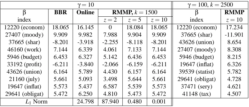
Finally, we present results of application of the algorithms to the RCV1-v2 data sets. For the

RCV1-v2 training data (d =47,236, t =23,149), sparsity again enables application of BBR to

obtain the batch MAPβparameter values, as well as the Online and MP algorithms, although this is

quite cumbersome. See Table 5. Again, as expected (examining d vs. t for this data set), the Online estimates are not very good. The multi-pass algorithms have improved parameter estimates. For

γ=10 (a fairly high amount of regularization), we find essentially the same qualitative results as

j BBR Online MP RMMP, k=300

z=3 z=5 z=3 z=5 z=7 Intercept -1.588 -1.404 -1.527 -1.586 -1.451 -1.573 -1.588

9 (bank) 1.188 0.697 0.957 1.185 0.688 1.143 1.188

13 (share) 0.847 0.609 0.793 0.846 0.678 0.839 0.847

147 (acquisit) 0.813 0.562 0.795 0.813 0.696 0.812 0.813

31 (offer) 0.801 0.337 0.618 0.800 0.356 0.772 0.801

..

. ... ... ... ... ... ... ...

3 (pct) -2.264e-2 -2.259e-2 -2.127e-2 -2.240e-2 -3.247e-2 -2.062e-2 -2.264e-2 62 (plan) -1.757e-2 -1.430e-2 -2.840e-2 -1.779e-2 -3.346e-2 -2.045e-2 -1.757e-2 2 (dlr) 1.552e-2 6.932e-3 1.542e-2 1.548e-2 1.610e-2 1.525e-2 1.552e-2 12 (net) -1.467e-2 -6.671e-3 -1.956e-2 -1.480e-2 -1.415e-2 -1.643e-2 -1.467e-2

8 (ct) 1.277e-2 3.587e-2 2.870e-2 1.320e-2 2.915e-2 1.776e-2 1.278e-2

L1Norm 4.029 1.691 0.034 3.496 0.4027 3e-4

Table 3: Results obtained on the ModApte data set. The 5 highest and 5 lowest magnitude non-zero

coefficients of MAPβforγ=100 are shown. In table are the indices ofβ(and word stem

features they correspond to in brackets), coefficients from BBR, and the Online algorithm, those obtained after a particular number of passes over the data using the MP algorithm

(full memory) and parameters from the RMMP algorithm with k=300.

j BBR Online RMMP, z=8

k=3120∗ k=2000 k=1000 k=600 k=300

292 (banker) 2.695 1.523 2.695 2.695 2.695 2.695 2.699

20 (4) 2.268 0.617 2.268 2.260 2.260 2.259 2.273

Intercept -2.010 -1.615 -2.010 -2.009 -2.009 -2.009 -2.005

341 (charg) 1.755 0.832 1.755 1.754 1.754 1.754 1.742

147 (acquisit) 1.572 0.862 1.572 1.572 1.572 1.572 1.568 ..

. ... ... ... ... ... ... ...

66 (loan) 4.943e-3 9.106e-2 4.944e-3 4.849e-3 4.821e-3 4.849e-3 3.224e-3 134 (agre) 4.488e-3 4.836e-2 4.479e-3 4.720e-3 4.756e-3 4.712e-3 1.677e-2 267 (commerci) -2.057e-3 0 -2.068e-3 -1.863e-3 -1.897e-3 -1.852e-3 -3.427e-3 28 (stock) -1.652e-3 -3.879e-2 -1.644e-3 -1.542e-3 -1.560e-3 -1.537e-3 -1.991e-3 56 (interest) -1.518e-4 -7.623e-2 -1.540e-4 -3.059e-4 -2.983e-4 -3.121e-4 -8.640e-4

L1Norm 28.290 1.4e-3 0.047 0.044 0.048 1.269

Table 4: Results for the ModApte data set: Illustrating the effect of changing k. The 5 highest

and 5 lowest magnitude non-zero coefficients of MAPβfor γ=10 are shown. In table

are the indices ofβ(and word stem features they correspond to in brackets), coefficients

from BBR, the Online algorithm, and those obtained after 8 passes over the data using the

γ=10 γ=100, k=2500

β BBR Online RMMP, k=1500 β RMMP

index z=2 z=5 z=10 index z=10

12220 (econom) 18.065 16.145 0 18.084 18.065 12220 (econom) 17.234 27407 (moody) 9.909 9.982 7.988 9.904 9.909 37665 (shar) -11.901

37665 (shar) -8.201 -3.918 -2.255 -8.118 -8.201 43626 (union) 8.654 46160 (work) 7.144 6.339 4.061 7.133 7.144 27407 (moody) 8.308 5946 (budget) 6.453 6.327 5.142 6.436 6.453 5946 (budget) 8.215 33192 (profit) -6.211 -3.840 -2.066 -6.159 -6.211 19647 (inflat) 6.326 43626 (union) 6.164 5.789 4.430 6.157 6.164 39539 (statist) 5.782 21160 (july) 5.661 5.093 3.498 5.644 5.661 29641 (obligat) 4.728 19647 (inflat) 5.573 5.437 6.587 5.539 5.573 37471 (sery) 4.621 29641 (obligat) 5.472 6.250 4.810 5.473 5.472 41148 (tax) 4.507

L1Norm 24.798 87.940 0.480 0.001

Table 5: RCV1-v2 results. Left portion RCV1-v2 training data set, right BIG-RCV data set.

parameter values as BBR (not shown in the table). The RMMP algorithm also gives excellent results

in about 10 passes, see the left portion of Table 5 with k=1500.

For the BIG-RCV data set (d =288,062, t =421,816) however, computational and memory

limitations made it impossible to run the batch algorithms on this data set (also the Online and MP algorithm). It is precisely for cases like this that the RMMP algorithm is useful, and we were able to obtain parameter estimates for reasonable settings of regularization—see for example, the right portion of Table 5.

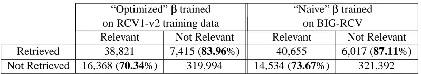
Does training on the entire BIG-RCV data set actually result in improved predictive perfor-mance? To address this, we conducted the following experiment. We obtained the best possible predictive parameters using 10-fold cross-validation on the RCV1-v2 training data set with a batch algorithm. This is an expensive computation, involving many repeated BBR runs for different val-ues of the regularization parameter (we searched over γ=0.01,0.1,1,10,100). The final

cross-validation chosenβhas 1010 non-zero parameters.

We then trained a separate sparse logistic classifier on the BIG-RCV data set using the RMMP

algorithm with k=3000 andγ=40. Setting γ=40 results in 1015 non-zero MAPβcoefficients

which is approximately the same number of non-zero coefficients as the cross-validation chosen

β. Finally, we compare the predictive accuracy of both classifiers on the unused RCV test set

(comprising the unused two portions of the original RCV1-v2 test data).

The results, shown in Table 6, demonstrate that using the information in extra examples, the “un-sophisticated” classifier trained on the much larger data set outperforms the “optimized” classifier trained on a smaller data set.

8. Conclusions

state-“Optimized”βtrained “Naive”βtrained

on RCV1-v2 training data on BIG-RCV

Relevant Not Relevant Relevant Not Relevant

Retrieved 38,821 7,415 (83.96%) 40,655 6,017 (87.11%)

Not Retrieved 16,368 (70.34%) 319,994 14,534 (73.67%) 321,392

Table 6: This table shows confusion matrices for prediction results on the RCV Test data set. The

CVβ (trained on the RCV1-v2 training data set) results are on the left and the MAPβ

(trained on the BIG-RCV data set, withγ=30, k=3000) results are on the right. Also

shown are recall and precision percentages in bold and brackets. There are approximately 383,000 examples in the test data set.

of-the-art batch algorithms are impractical/cumbersome, and our results show that examining such data sets in their entirety can lead to better classifier performance.

Some areas of further research that this work opens up are: extension of the algorithms for a hi-erarchical prior model so that the choice of regularization is less important, the possible application of our methods to kernel classifiers, and applications to multi-class classification problems.

Acknowledgments

National Science Foundation grants IIS-9988642 and DMS-0505599 and the Multidisciplinary Re-search Program of the Department of Defense (MURI N00014-00-1-0637) supported this work. We are very grateful to David D. Lewis for detailed and insightful comments on an earlier draft of this paper.

Appendix A.

Here we show the Taylor expansions for the quadratic approximations to the log-likelihood function. To simplify notation, let c(β) =βTxiand ˆc=βTi₋1xi. The link function (we will restrict analytical

results to the logistic and probit link functions) isΦ(z)as before and we denote its first and second derivative, with respect to z, byΦ0(z)andΦ00(z)respectively.

Consider the case where yi=1:

logΦ(c) _≈ logΦ(cˆ) + (c₋cˆ)Φ_Φ0(cˆ) (cˆ) +

(c−cˆ)2

2

Φ00_(cˆ) Φ(cˆ) −

Φ₀ (cˆ)

Φ(cˆ) 2!

∝ Φ0(cˆ) Φ(cˆ)c+

1 2

Φ00_(cˆ) Φ(cˆ) −

Φ₀ (cˆ)

Φ(cˆ) 2!

c2₋cˆ Φ

00_(cˆ) Φ(cˆ) −

Φ₀ (cˆ)

Φ(cˆ) 2!

c

so that:

ai=

1 2

Φ00_(cˆ) Φ(cˆ) −

Φ₀ (cˆ)

and

bi= Φ0_(cˆ)

Φ(cˆ) −cˆ

Φ00_(cˆ) Φ(cˆ) −

Φ₀ (cˆ)

Φ(cˆ) 2!

.

Analogously, when yi=0:

log(1₋Φ(c))_≈log(1₋Φ(cˆ))₋(c₋cˆ) Φ0(cˆ)

1₋Φ(cˆ)−

(c₋cˆ)2

2

Φ00_(cˆ)

1₋Φ(cˆ)+ Φ0

(cˆ)

1₋Φ(cˆ) 2!

so that:

ai=−

1 2

Φ00_(cˆ)

1₋Φ(cˆ)+ Φ0

(cˆ)

1₋Φ(cˆ) 2!

and

bi=− Φ0_(cˆ)

1₋Φ(cˆ)+cˆ

Φ00_(cˆ)

1₋Φ(cˆ)+ Φ₀

(cˆ)

1₋Φ(cˆ) 2!

.

For the probit link function:

Φ(z) =

Z z

−∞

1

√

2πe

−x2_/2 dx

Φ0_{(z) = √}1

2πe

−z2/2

Φ00_{(z) = √}−z

2πe

−z2_/2

,

whereas for the logistic link function:

Φ(z) = e z

1+ez Φ0_{(z) =} ez

(1+ez₎2

Φ00_{(z) =} (ez)(1−ez) (1+ez₎3 .

These expressions then allow us to compute the ai,bi in the cases needed.

Appendix B.

In this appendix we derive the modified Shooting algorithm, Algorithm 1 and discuss its efficient implementation. We derive Shooting by analyzing the subdifferential of the system (Rockafel-lar, 1970). We need convex smooth analysis results because the regularization term is

non-differentiable at zero. Reviewing concepts very briefly, the subgradientξ∈R|x|_{, of a convex}

func-tion f at x0is defined to be any vector satisfying:

f(x)_≥ f(x0) +ξT(x₋x0).

In words, any vector ξ, such that a plane through (x,f(x))with slope ξ contains f in its upper

f ). The subdifferential, ∂f , is just the set of all subgradients, ξ, at a particular point. This is a generalization of the gradient which collapses to the gradient, whenever f is differentiable. As

a simple example, the subdifferential of f(β) =_|β_|, the absolute value function (which is

non-differentiable atβ=0) is:

∂f =  



{−1_}, β<0 [₋1,1], β=0

{1}, β>0.

As one expects, analogous to optimality conditions resulting from setting the gradient of a differen-tiable function to zero, optimality conditions for non-differendifferen-tiable functions result from restrictions on the subdifferential. In particular we appeal to the following result from non-smooth analysis (Rockafellar, 1970):

Theorem ˆβis a global minimizer of a convex function f(β)if and only if 0∈∂f(βˆ).

Now to our particular problem. We need to findβthat is a solution to:

max β

βT_Ψβ

+βTθ₋γ_kβ_k1

.

The convexity of the problem allows us to make incremental progress towards the maxima coordinate-wise. Starting from some parameter vector, we compute the jth component of the subdifferential of the function (keeping all other components fixed):

∂ ∂βj(β

T_{Ψβ) +} ∂

∂βj(β T_θ)

−γ∂(∑d

j=1(|βj|)

= 2(Ψβ)j+θj−γ∂(|βj|)

= 2Ψj jβj+2(Ψ0β)j+θj−γ∂(|βj|)

where (Ψ0β)j is the j’th component of the vector Ψ0β andΨj j refers to the (j,j)’th element of

the matrixΨ(Recall thatΨ0 is defined to be the matrixΨwith diagonal entries set to zero). The

second equation follows from the first as the subdifferential of a univariate differentiable function

is just its derivative and since matrixΨis symmetric (it is just a weighted sum of outer products).

Now if we plug in the subdifferential of the non-differentiable absolute value function, and set

Ωj =2(Ψ0β)j+θj (and thus define the vector Ω to be the gradient of the purely differentiable

part of the objective function), we obtain the subdifferential of the objective function, whose j’th

component we denote by∂_βj as:

∂βj =  



{2Ψj jβj+Ωj +γ}, βj<0

[Ωj −γ,Ωj +γ], βj=0

{2Ψj jβj+Ωj −γ}, βj>0.

This is a piecewise linear function with fixed negative slope 2Ψj jand a constant jump of fixed size

2γatβj=0 (Ψj jcan be proven to always be negative by looking at the update formula forΨand

using the fact that_∀i,ai<0). Using the optimality criteria (now for maximization since−|βj|is a

concave function) naturally leads to the modified Shooting algorithm, illustrated in Figure 6. Now to questions regarding the efficient implementation of the Shooting algorithm, used by the online, MP and RMMP algorithms. In the modified Shooting algorithm, after each component

update (change in βj) we need to modify Ω(the update Ωstep in the algorithm). This can be

implemented efficiently using the following result (similar to the trick detailed in Minka, 2001):

Ωnew_=Ωold_+2Ψ0

0

0 βj=0

Ω_j + γ

Ω_j − γ

β_j ∂_β

j

(a)

0 0

β_j<0

Ω_j + γ <0

Ω_j − γ

β_j ∂_β

j

(b)

0 0

β_j>0 Ω_j + γ

Ω_j − γ >0

β j ∂_β

j

(c)

Figure 6: Illustration of cases occurring in the Shooting algorithm (a) If_|Ωj| ≤γthe constant

por-tion of the subdifferential contains zero. In this case, setβj=0 (b) If instead,Ωj<−γ,

the optimality conditions will be satisfied by settingβj =−₂γ_Ψ−Ω_{j j}j (c) The case analogous

where∆βj is the change in βj andΨ0_(.j) is the j’th column of Ψ0. Thus each component update

of Shooting can be done in O(d)computational time. Now, if as before the maximum number of

non-zero components ofβalong the solution path to MAPβis m, only m such updates will need to

be made, giving a total time requirement per iteration of O(md).

Finally we detail how to carry out the Ωupdates efficiently for the RMMP algorithm,

Algo-rithm 3. Recall that since we are discussing a multi-pass algoAlgo-rithm, the location where we take the

quadratic approximation, β_i−1, is constant throughout the pass through the fixed data set, Dt. We

exploit this fact to show that in this case, you don’t explicitly need the matrixΨ(or ˜Ψ) to determine

Ω. Indeed, after going through all the observations in the data set (pass z, say):

Ω=2Ψ0β_z−1+θ=2

t

∑

ai xixTi −diag(x2i)

! β_z−1+

t

∑

bixi,

which follows from the definitions ofΩ,θandΨ0. In the above equation, diag(x2

i)is a d×d matrix

zero everywhere except the diagonal entries, which consists of the elements of the vector xisquared

component-wise. This leads to the following equation forΩ:

Ω=2

t

∑

ai(βTz−1xi)xi−2 t

∑

ai(x2iβz−1) + t

∑

bixi,

where(x2

iβz₋1)is a vector whose entries are x2i multiplied byβz₋1component-wise. Note the first

sum is just a weighted combination of the input data (βT_z−1xi is a scalar). Thus, our final update

formula results:

Ωnew_=Ωold_{+ (2a}

iβTz₋1xi+bi)xi−2ai(x2iβz₋1).

As can be seen, computing this update per observation takes time and space O(d), and having

restricted the number of non-zero components ofβto k, a total computational cost per iteration of

Shooting to O(kd).

Appendix C.

We present a proof sketch for the convergence behavior of the online algorithm in the infinite data

limit. The intuition for is as follows: as t _→∞, the Bayesian central limit theorems dictate that

the posterior distribution tends (in distribution) to a multivariate Gaussian with ever shrinking co-variance, (Bernardo and Smith, 1994). Thus, less and less information is required to encode the posterior distribution as more and more data is added—to a point. Indeed, in the limit, only the

vector of the maximum likelihood value of the parameters,β_MLE, is required to completely describe

the posterior distribution.

Suppose now that the online algorithm converges to a particular fixed point. In the infinite data limit, an infinite number of term approximations are taken at this fixed point. Now, our Taylor polynomial based approximation preserves both the function value and its gradient, and an infinite number of approximations are jointly maximum at this fixed point. This implies the fixed point is an optima of the posterior distribution.

a theorem in Opper (1998). Even though Opper derives his results based on a Gaussian prior on

the parametersβ(corresponding to L2regularization), the general format of Opper’s theorem is still

applicable in our case because, in the infinite data limit, the prior is inconsequential.

References

J. M. Bernardo and A. F. M. Smith. Bayesian Theory. John Wiley and Sons, Inc., 1994.

S. S. Chen, D. L. Donoho, and M. A. Saunders. Atomic decomposition by Basis Pursuit. SIAM Journal on Scientific Computing, 20(1):33–61, January 1999.

B. Efron, T. Hastie, I. Johnstone, and R. Tibshirani. Least angle regression. The Annals of Statistics, 32(2):407–499, 2004.

E. Eskin, A. J. Smola, and S.V.N. Vishwanathan. Laplace Propagation. In Neural Information Processing Systems, 16. MIT Press, 2003.

M. A. T. Figueiredo and A. K. Jain. Bayesian learning of sparse classifiers. In Proceedings of the Computer Vision and Pattern Recognition Conference, volume 1, pages 35–41, 2001.

W. J. Fu. Penalized regressions: The Bridge versus the Lasso. Journal of Computational and Graphical Statistics, 7(3):397–416, 1998.

A. Genkin, D. D. Lewis, and D. Madigan. Large-scale Bayesian logisitic regression for text catego-rization. Technometrics, 49:291–304, 2007.

T. Hastie, S. Rosset, R. Tibshirani, and J. Zhu. The entire regularization path for the Support Vector Machine. Journal of Machine Learning Research, 5:1391–1415, 2004.

T. Jaakkola and M. Jordan. Bayesian parameter estimation via variational methods. Statistics and Computing, 10:25–37, 2000.

R. E. Kass and A. E. Raftery. Bayes factors. Journal of the American Statistical Association, 90: 773–795, 1995.

K. Koh, S.-J. Kim, and S. Boyd. An interior-point method for large-scale l1-regularized logistic

regression. Journal of Machine Learning Research, 8:1519–1555, 2007.

P. Komarek and A. Moore. Making logistic regression a core data mining tool: A practical in-vestigation of accuracy, speed, and simplicity. Technical Report TR-05-27, Robotics Institute, Carnegie Mellon University, Pittsburgh, PA, May 2005.

B. Krishnapuram, L. Carin, M. A. T. Figueiredo, and A. J. Hartemink. Sparse multinomial logistic regression: Fast algorithms and generalization bounds. IEEE Transactions on Pattern Analalysis and Machine Intelligence, 2005.

D. D. Lewis. Reuters-21578 text categorization test

collec-tion: Distribution 1.0 readme file (v 1.3)., 2004. URL

D. D. Lewis, Y. Yang, T. G. Rose, and F. Li. RCV1: A new benchmark collection for text catego-rization research. Journal of Machine Learning Research, 5:361–397, 2004.

D. J. C. MacKay. Probable networks and plausible predictions: a review of practical Bayesian methods for supervised neural networks. Network: Computation in Neural Systems, 6:469–505, 1995.

T. P. Minka. Expectation Propagation for approximate Bayesian inference. In Jack Breese and Daphne Koller, editors, Proceedings of the Seventeenth Conference on Uncertainty in Artificial Intelligence (UAI-01), pages 362–369, San Francisco, CA, August 2–5 2001a. Morgan Kauf-mann Publishers.

T. P. Minka. A Family of Algorithms for Approximate Bayesian Inference. PhD thesis, Massachusetts Institute of Technology, Dept. of Electrical Engineering and Computer Science, 2001b.

M. Opper. A Bayesian approach to on-line learning. In D. Saad, editor, Online Learning in Neural Networks, pages 363–378. Cambridge University Press, 1998.

M. R. Osborne, B. Presnell, and B. A. Turlach. A new approach to variable selection in least squares problems. IMA Journal of Numerical Analysis, 20(3):389–403, July 2000.

Y. Qi, T. P. Minka, R. W. Picard, and Z. Ghahramani. Predictive automatic relevance determination by Expectation Propagation. In Proceedings of Twenty-first International Conference on Machine Learning, Banff, Alberta, Canada, July 4-8 2004.

R. T. Rockafellar. Convex Analysis. Princeton University Press, Princeton, N.J, 1970.

S. K. Shevade and S. S. Keerthi. A simple and efficient algorithm for gene selection using sparse logistic regression. Bioinformatics., 19(17):2246–2253, 2003.

R. J. Tibshirani. Regression shrinkage and selection via the Lasso. Journal of the Royal Statistical Society, Series B, 58(1):267–288, 1996.

T. Zhang. On the dual formulation of regularized linear systems. Machine Learning, 46:91–129, 2002.

T. Zhang and F. J. Oles. Text categorization based on regularized linear classification methods. Information Retrieval, 4(1):5–31, 2001.