Classifying With Confidence From Incomplete Information
Nathan Parrish [email protected]
Applied Physics Laboratory Johns Hopkins University Laurel, MD 20723, USA
Hyrum S. Anderson [email protected]
Sandia National Laboratories Albuquerque, NM 87123, USA
Maya R. Gupta [email protected]
1225 Charleston Rd Google Research
Mountain View, CA 94025, USA
Dun Yu Hsiao [email protected]
Department of Electrical Engineering University of Washington
Seattle, WA 98195-4322, USA
Editor:Kevin Murphy
Abstract
We consider the problem of classifying a test sample given incomplete information. This problem arises naturally when data about a test sample is collected over time, or when costs must be incurred to compute the classification features. For example, in a distributed sensor network only a fraction of the sensors may have reported measurements at a certain time, and additional time, power, and bandwidth is needed to collect the complete data to classify. A practical goal is to assign a class label as soon as enough data is available to make a good decision. We formalize this goal through the notion of reliability—the probability that a label assigned given incomplete data would be the same as the label assigned given the complete data, and we propose a method to classify incomplete data only if some reliability threshold is met. Our approach models the complete data as a random variable whose distribution is dependent on the current incomplete data and the (complete) training data. The method differs from standard imputation strategies in that our focus is on determining the reliability of the classification decision, rather than just the class label. We show that the method provides useful reliability estimates of the correctness of the imputed class labels on a set of ex-periments on time-series data sets, where the goal is to classify the time-series as early as possible while still guaranteeing that the reliability threshold is met.
Keywords: classification, sensor networks, signals, reliability
1. Introduction
raw data to produce a full set of classification features. Thus, it is desirable to know if one can make a good decision without collecting all of the test data. Specifically, we wish to guarantee that a decision made from incomplete test data has a high probability of being the same decision that would be made given the complete test data.
In this paper, we focus on answering the question “With probability at least equal toτ, will the classification decision from incomplete data be the same as that which would be made from the complete data?” Our approach also makes it possible to answer the related question, “If we classify based on the current incomplete data, what is the probability that the class decision will be the same as classifying from the complete data?”
First, we propose optimal and practical decision rules for classifying incomplete data. In Sec-tions 3, 4, and 5 we provide the details on how to efficiently and accurately implement the proposed practical decision rule for classifiers that use linear or quadratic discriminants, such as linear sup-port vector machines and linear or quadratic discriminant analysis (LDA and QDA). In Section 6, we review related work on classifying with missing features and related work on early classification of time-series data. Experiments in Section 7 show that the proposed incomplete decision rule con-sistently provides enhanced reliability over the state of the art in classifying incomplete data. We further discuss the results and some open questions in Section 8.
This paper significantly extends our prior work in the conference paper (Anderson et al., 2012), where we tackled the same problem but proposed a more conservative decision rule. In this paper, we propose a more tractable decision rule, show how it can be used with different kinds of classifiers, show that our approach can be applied to different features, and provide substantially more analysis and experimental results.
2. Incomplete Decision Rules
Let ˆg(x)be a classifier function that assigns a class label to test samplex. However, suppose that at test time we do not havex, but instead have some incomplete information given as a vectorz. We wish to classifyzif it gives us enough information aboutxto make a good decision, otherwise, we delay making a decision until we have more information. To that end, we consider decision rules that answer the question: “Can we classify zand know that we meet some minimum probability threshold of making the same decision that we would make onx?” We use the termreliabilityto mean the probability that the class label assigned tozmatches that assigned tox.
To estimate reliability, we model the classification features derived from the complete data as a random variableX, whereX is jointly distributed with the random variableZmodeling the incom-plete data. Given a desired reliabilityτ∈[0,1]and a realization of the incomplete informationz, an ideal incomplete decision rule is to classify as classgif
P(gˆ(X) =g|Z=z) = Z
xs.t.gˆ(x)=g
p(x|z)dx
≥τ, (1)
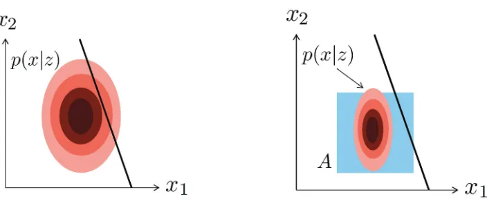
and otherwise to wait for more information. Figure 2 illustrates this rule.
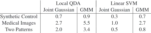
Figure 1: In this example, the available information is the incomplete time signalz, shown in green. Assuming the complete signal is iid with the training signals, the complete signal can be treated as a random signal (illustrated in pink), implying a conditional density on the complete signal’s classification features, p(x|z). Given p(x|z) we can check whether or not one can make a reliable classification.
and see if ˆg(x)maps allxin one such set to a single classg. In general, we expect both these checks to be computationally intractable.
We propose that a more conservative, but computable, incomplete decision rule is to classify as classgif
ˆ
g(x) =g for all x∈Afor some setAsuch thatP(X∈A|Z=z)≥τ. (2) Rule (2) differs from (1) in that only one setAthat contains at leastτmeasure ofXmust be checked. This rule is more conservative than (1) because it does not check all setsA, and thus (1) could be satisfied without (2) being satisfied (but not vice-versa).
Implementing the proposed rule given in (2) requires three steps. First, we must estimate the conditional density p(x|z). Second, we must construct an appropriate set A, and third, we must check if the rule is satisfied. We first discuss the construction of a setAin Section 3, and show that our construction only requires estimates of the first and second conditional moments ofX. Then in Section 4, we show how rule (2) can be efficiently checked for classifiers that have linear or quadratic class discriminant functions. We delay the discussion of how to estimate the necessary moments ofXuntil Section 5.
3. Defining a SetAthat Contains MeasureτofX
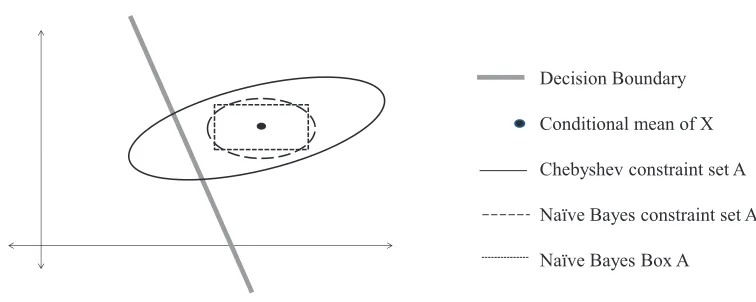
To implement the incomplete decision rule (2), one must be able to construct a setAthat contains at leastτmeasure ofXgivenz. In this section we propose three ways to construct such a setA. Figure 3 compares these three constructions.
3.1 Chebyshev Construction for SetA
Figure 2: Comparison of the ideal and proposed conservative but computable decision rule. Left: A two-dimensional feature space and a linear class decision boundary. The probability mass ofX lies mostly to the left of the decision boundary. For desired reliability valuesτ that are smaller than the probability mass ofXthat falls to the left of the decision bound-ary, the ideal incomplete decision rule would choose to classify based on the incomplete informationz. Right:The entire probability mass of X falls on one side of the decision boundary, and thus the ideal incomplete decision rule would choose to classify rather than wait, for every value ofτ. However, our computable incomplete decision rule constructs a setAthat captures a fractionτof the mass ofXand requires that entire setAto lie on one side of the decision boundary. For the choice ofAshown here in blue, the setAcrosses the decision boundary, and thus the computable decision rule would choose to wait for more information before classifying.
be constructed using the multidimensional Chebyshev inequality, which states that forX∈Rdwith known meanmand covarianceR, and anyα>0:
P (X−m)TR−1(X−m)≤α2
≥1− d
α2. Thus to satisfyP(X∈A|Z=z)≥τ, define
A=
xs.t.(x−m)TR−1(x−m)≤ d 1−τ
. (3)
The setAdefined by (3) is non-empty forτ∈(−∞,1], althoughτ≤0 does not give a useful bound for the incomplete classifier reliability.
3.2 Naive Bayes Constructions for SetA
Decision Boundary
Conditional mean of X
Chebyshev constraint set A
Naïve Bayes constraint set A
Naïve Bayes Box A
Figure 3: Example sets that contain mass τ of the conditional p.d.f. of X formed by the three different construction methods forAproposed Section 3.
For example, if we assume that the conditional distribution is Gaussian,1then a quadratic setAthat coversτmeasure ofX is
A=
x s.t. (x−m)TR−1(x−m)≤erf(τ) , (4) where one must compute the inverse cdf to determine the value erf(τ) to achieve a set A with measureτ. For a multi-dimensional Gaussian, computing the inverse cdf for (4) is non-trivial. We can simplify (4) by making the conservative n¨aive Bayes assumption that the components ofX are independent, and thusRis diagonal. Then the quadratic function in (4) becomes∑dℓ=1
x√(ℓ)−m(ℓ)
R(ℓ,ℓ)
2
.
Under the independent Gaussian assumption,∑dℓ=1
X√(ℓ)−m(ℓ)
R(ℓ,ℓ)
2
is a chi-squared random variable withddegrees of freedom; thus, the erf(τ)function in (4) is easily computed using the inverse cdf of a chi-squared random variable.
A related option is to force the setAto be a box. Again, make the n¨aive Bayes assumption that elements ofX are independent, thenp(x|z) =∏ℓd=1p(x(ℓ)|z). Therefore, we can define a set
A={xs.t.x(ℓ)∈[m(ℓ)−sτ(ℓ),m(ℓ) +sτ(ℓ)]∀ℓ=1, ...,d}, (5)
wheresτis a vector defining the width of the box in each dimension such that the total measure of
the box isτ. In this paper, we implement this constraint by assigning each dimension equal measure τ1/d while assume that each marginal distributionX(ℓ)is Gaussian.
The two options (4) and (5) make the same two assumptions about the conditional distribution ofX, but (4) finds the ellipsoidal footprint of the Gaussian that has measureτ, while (5) treats the dimensions completely independently, giving each of the marginals measureτ1/d.
4. Efficient Solutions for Linear or Quadratic Discriminants
In this section, we show that the incomplete data classification rule (2) with the constraint setsA
proposed in Section 3 can be computed efficiently for classifiers of the form ˆ
g(x) =arg max
g
fg(x), (6)
where fg(x)is a linear or quadratic discriminant function for thegthclass, and according to (6), the
classifier assignsx to the class with the maximum discriminant. For example, the linear support vector machine (SVM) has a linear discriminant, while the quadratic discriminant analysis (QDA) classifier has a quadratic discriminant (Hastie et al., 2001).
Nearest-neighbor classifiers using an Euclidean (or Mahalanobis) distance have a discriminant that over the setx∈Arequires taking the minimum of a set of quadratic discriminants:
fg(x) = min xi:yi=g
(x−xi)T(x−xi).
An optimal method for checking the incomplete decision rule (2) for this discriminant is an open question. A conservative reliability decision can be made by treating each sample as its own class in (6). That is, let fi(x) = (x−xi)T(x−xi), solve (6) for the resulting quadratic discriminant, and
then classify as the classyi. A computationally simpler approach (but one that is not strictly
con-servative), is to only consider each class’s nearest neighbor to the posterior mean, which produces one quadratic discriminant per class. In experiments, we do something similar to the latter approach using a local QDA classifier.
We begin with the two-class problem, and then show how this rule can be extended to multi-class problems.
4.1 Two-class Problems
We first consider a two-class problem, where the set of class labels is
G
={1,2}. Let f1(x)andf2(x)be the discriminants for classes one and two, and define
f(x) = f2(x)−f1(x).
We can define an equivalent classifier to (6) using only f(x) by noting that f(x) =0 defines the decision boundary between classes 1 and 2. Therefore, classification rule (6) is equivalent to
ˆ
g(x) =
1 if f(x)≤0 2 if f(x)>0.
Then the proposed incomplete data decision rule (2) is implemented:
ˆ
g(z) =
1 if max
x∈A f(x)≤0
2 if min
x∈A f(x)>0
no decision otherwise.
(7)
Note that the decision rule (7) is dependent on the incomplete data through the dependence ofAon
−2 −1 0 1 2 −2
−1 0 1 2
Decision Boundary Mean of X Boundary of A
−2 −1 0 1 2
−2 −1 0 1 2
−2 −1 0 1 2
−2 −1 0 1 2
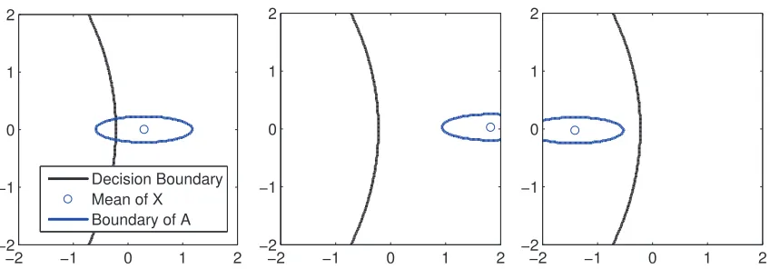
Figure 4: Three different scenarios for incomplete data classification. In the leftmost plot, the clas-sifier withholds making a decision. In the center and rightmost plots,Alies completely on a single side of the decision boundary, so the classifier assigns a label to the incomplete data.
4.1.1 LINEARDISCRIMINANTS
In order to efficiently check (7), we must be able to efficiently compute the maximum and minimum of f(x) over the set x∈A. If f1(x) and f2(x) are linear discriminants, then f(x) is also linear. Coupled with a quadratic set A, such as the Chebyshev or n¨aive Bayes quadratic setsA given in Section 3, finding the maximum and minimum are the linear programs with quadratic constraints:
max
x∈A f(x) =maxx β
Tx+b (8)
s.t.(x−m)TR−1(x−m)≤δ
min
x∈A f(x) =minx β
Tx+b (9)
s.t.(x−m)TR−1(x−m)≤δ.
These optimizations have closed-form solutions: Proposition 1:The solutions to (8) and (9) are, respectively
max
x∈A f(x) =β
Tm+√δ
kR1/2βk2+b
min
x∈A f(x) =β Tm
1e−300 1e−10 1e−5 0.001 0.1 200
400 600 800 1000
Reliability Requirement
Run Time (s) SDP
Gradient Descent
0 10 20 30 40 50
95 96 97 98 99 100
Average Classification Time
Reliability
SDP
Gradient Descent
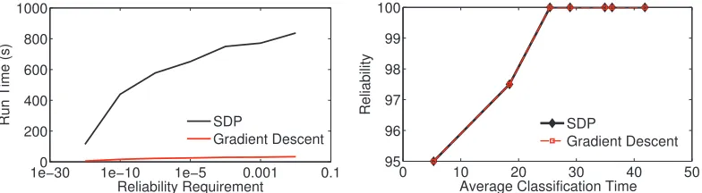
Figure 5: The left figure shows the time required by the SDP vs gradient descent solutions. The right figure verifies that the solution for the methods is identical.
For a linear set Asuch as the n¨aive Bayes box constraint set given in (5), the maximum and minimum are:
max
x∈A f(x) =maxx β
Tx+b (10)
s.t.m(ℓ)−sτ(ℓ)≤x≤m(ℓ) +sτ(ℓ)∀ℓ=1, ...,d
min
x∈A f(x) =minx β
Tx+b (11)
s.t.m(ℓ)−sτ(ℓ)≤x≤m(ℓ) +sτ(ℓ)∀ℓ=1, ...,d.
The solution of (10) isβTm+|βT|s
τ+b, and the solution of (11) isβTm− |βT|sτ+b.
4.1.2 QUADRATICDISCRIMINANTS
If the class discriminant functions are quadratic, then f(x) = f2(x)−f1(x) will also be quadratic and, thus, can be written
f(x) = (x−v)TV(x−v) +b. (12) Since (12) is the difference of two quadratics,V will generally be indefinite even if f2(x)and f1(x) are both positive semi-definite.
Now consider finding the maximum and minimum of (12) over the box set A. An efficient solution is obtained by first performing a change of variables that diagonalizesV. Definey=V1/2x
andw=V1/2v, then f(x) = f(y) =ky−wk2+b. After this change of variables, we can greatly simplify the maximum and minimum computations required by the incomplete decision rule (7) by making the n¨aive Bayes assumption on the random variableY =V1/2X as opposed to onX. Defining the mean ofY asmy=V1/2m,
max
x∈A f(x) =maxy∈A ky−wk
2+b (13)
min
x∈A f(x) =miny∈A ky−wk
2+b, (14)
with
A={ys.t.y(ℓ)∈[my(ℓ)−sτ(ℓ),my(ℓ) +sτ(ℓ)],∀ℓ=1, ...,d},
where thesτ(ℓ)are determined by the inverse cdf ofY(ℓ).
After this change of variables, theythat maximizes (13) is found by assigning eachy(ℓ)to the edge of the box that maximizes the distance fromw(ℓ). Similarly, theythat minimizes (14) assigns
y(ℓ) =w(ℓ)ifw(ℓ)∈[my(ℓ)−sτ(ℓ),my(ℓ) +sτ(ℓ)]. Otherwise,y(ℓ)is assigned to the edge of the
box that minimizes the distance tow(ℓ). 4.2 Multi-class Classifiers
We now extend the results of the previous section to multi-class classifiers. For multi-class classi-fiers, the classification rule (6) can be expressed:
ˆ
g(x) =c if fc(x)−fh(x)≥0 for all h6=c.
The proposed incomplete data classification rule (2) can be written: ˆ
g(z) =
(
c if min
x∈A fc(x)−fh(x)≥0 for allh6=c
no decision otherwise. (15)
That is, classifyzas classcif the setAlies completely within the decision region for some classc, and do not decide at the requested reliability if the setAstraddles a decision boundary.
If there areGtotal classes, then (15) implies 2 G2possible checks of the form minx∈A fc(x)− fh(x)≥0. However, we show in the next section that regardless of the construction of setA, one
must compute at most 2(G−1) of these checks. Furthermore, if the setA contains the posterior meanm(as it does in all of our proposed constructions forA), then a decision can be made with at mostG−1 checks using this two-step procedure:
Step 1 - Guess:Letc=arg max
g fg(m).
Step 2 - Check: Sequentially check if minx∈Afc(x)−fh(x)≥0 forh=1,2, . . . ,G, h6=c. If the
check fails for any h, stop, and output the resultno decision. If the check holds for all h, then classify early as classc.
4.3 General Multiclass Decision Process
We provide a provably efficient multi-class decision process for arbitrary constructions of the con-straint set A. We say that classc dominatesclass hand that classhis dominated byc if fc(x)− fh(x)≥0 for allx∈A. If neither class dominates the other one, then the two classes are calledtied.
4.3.1 PROPOSEDDECISIONPROCESS
Initialize:Begin with allGclasses labelledcandidate.
Compare:Choose any two classescandhthat are labelledcandidateand check if minx∈Afc(x)− fh(x)≥0. If yes, then label h as dominated. If no, then perform a second check to see if
minx∈A fh(x)−fc(x)≥0, and if so then labelc asdominated, and otherwise label both classes
astied. Continue this process until fewer than two classes are labelledcandidate. If no classes remain that are labelledcandidate, then output no decision. If one class is labelled candidate, then proceed to theFinal Comparison.
Final Comparison:Check if the last class labelledcandidatedominates every class labelledtied. If yes, classify the incomplete data as the class labelledcandidate, if no, outputno decision. Proposition 2: The above decision process correctly determines the dominating class or that there is no dominating class.
Proposition 3: Given G classes, the above decision process requires at most 2(G−1) minimum problem calculations evaluations, and at least G− ⌊G/2⌋pairwise evaluations.
5. Estimation of the Complete Test Data Distribution
In order to construct the setsAin Section 3, we must estimate the meanmand covarianceRof the complete test data X. We do this by leveraging the incomplete information about the test signal that is currently available along with the prior knowledge of the structure of the test signal gained from the training data using the standard assumption that the training and test features are IID. We present two estimation methods: 1) joint Gaussian estimation, and 2) Gaussian mixture model (GMM) estimation. These approaches are similar to those used in missing feature imputation, for example in speech recognition as described by Raj and Stern (2005). However, our approach differs from that of missing feature imputation in that the latter constructs only a point estimate of the unknown data, whereas we construct estimates of the mean and covariance of the unknown data.
5.1 Joint Gaussian Estimation
For joint Gaussian estimation, we assume that the complete dataX is distributed jointly Gaussian with the incomplete dataZ. Therefore, the model is
X Z
∼
N
¯
x
¯
z
,
Σx,x Σx,z
Σz,x Σz,z
. (16)
We estimate the model parameters in (16) from the training data. The mean and covariance param-eters ofXconditioned on the realization of the partial informationZ=zare
m=xˆ¯+Σˆx,zΣˆ−z,z1(z−zˆ¯) R=Σˆx,x−Σˆx,zΣˆ−z,z1Σˆz,x. 5.2 GMM Based Estimation
distributions. Under these assumptions the model is
X Z
∼
∑
g∈G w(g)P
X Z
g
, (17)
wherew(g)is the weight of the classgGaussian and
P
X Z
g
=
N
¯
xg
¯
zg
,
Σx,x(g) Σx,z(g)
Σz,x(g) Σz,z(g)
.
We can again estimate the parameters of the model (the means, covariances, and weights), from the training data.
Define
mg=xˆ¯g+Σˆx,z(g)Σˆ−z,z1(g)(z−zˆ¯g), Rg=Σˆx,x(g)−Σˆx,z(g)Σˆ−z,z1(g)Σˆz,x(g), p(g|z) =p(G=g|Z=z)
= wgp(Z=z|G=g)
∑h∈Gwhp(Z=z|G=h)
.
Given a realizationZ=z, we can compute the meanmofX as:
m=E[X|z] =
∑
g∈GE[X,G|z] =
∑
g∈Gmgp(g|z).
Furthermore, as shown in Appendix C, the covariance ofXis
R=
∑
g∈G
p(g|z) Rg+mgmTg
−
∑
q∈Gh
∑
∈GmqmThp(q|z)p(h|z).
6. Related Work
We detail the related work in early classification and missing features, then we contrast the proposed with optimal stopping, feature selection, online and incremental learning, and sequential hypothesis ratio testing.
6.1 Other Early Classification Work
Xing et al. (1998) considered the problem of making an early prediction on time-series data that matches that of a full length one nearest-neighbor classifier. Suppose that the labelled training data set is{(xi,gi)}ni=1, wherexi∈Rd. Their approach, called early classification on time-series (ECTS),
is motivated by the idea of theminimum prediction length(MPL) of a training time-seriesxi. Define xi(1 :t)∈Rt to be the firstt samples of xi. Furthermore, define, RNN(xi(1 :t))to be the reverse
nearest neighbors ofxi(1 :t)which is the set of training samples that choosexi to be their nearest
neighbor at time t. The MPL of xi is the smallest time index k such that for all k≤ℓ≤d the
following holds RNN(xi(1 :ℓ)) =RNN(xi(1 :d))6= /0. By this definition, the MPL is the smallest
revealed. At test time, a training pointxican be used to assign a label to a test samplex(1 :t)once t≥MPL(xi), the minimum prediction length ofxi.
The authors found that the above procedure was too conservative; therefore, they proposed a slightly modified way to find the MPL for ECTS. They first clustered the training data using a hierarchical clustering method and then selected the MPL for each training time-series depending on its cluster membership. They also introduced a parameter to control the earliness of their approach calledminimum support—a ratio that varies between zero and one, with zero resulting in the earliest classifier. However, the minimum support parameter is different from ourτparameter in that it does not provide an explicit guarantee on the reliability of the early decision.
Xing et al. cite Rodriguez and Alonso (2002) as the only existing study mentioning early clas-sification on time-series data. Rodriguez and Alonso (2002) propose to classify a time-series using aliteralbased classifier, where a literal is a descriptor describing what happens during a specified interval of the time-series. For example, the literalincreaseswould be set to one if the time-series increases during the specified interval, and would be set to zero otherwise. The authors mention that for early classification of time-series some of the literals will not yet have a value because the interval that they are measured in has not occurred yet. The authors propose to omit these literals from the classifier in order to classifier early.
6.2 Related Work on Missing and Noisy Features
Another related body of work is imputing (estimating) missing features. If missing features occur in the training data, then standard methods of classifier training cannot be used. One method of dealing with this problem, called single imputation, is to fill in the missing features with their estimated values. The missing features can be estimated using a multivariate regressor that is trained using the subset of training data with no missing features. Schafer and Graham (2002) and Rogier et al. (2006) review missing feature methods for training data.
When features are missing in the test data, there are three standard options (see, e.g., Saar-Tsechansky and Provost, 2007): imputing a point estimate for the missing features, imputing a distribution for the missing features, and the reduced-models approach. For the reduced models approach, classifiers are trained for each set of potentially missing information (Friedman et al., 1996; Schuurmans and Greiner, 2007; Saar-Tsechansky and Provost, 2007). Here, we do impute a distribution over the missing features (conditioned on the given information about the test sample and the training data statistics), but rather than just use that distribution to predict the best class label, we use the distribution to measure the reliability of a classification decision with the incomplete data. Thus, our contributions are in-part complementary to imputation methods, and different methods than the ones we used in Section 5 can be easily substituted into the proposed approach.
If features are noisy rather than missing, then estimating the clean feature values can improve test accuracy. This problem arises, for example, in automatic speech recognition (ASR) systems when the test signal is masked by noise (Cooke et al., 2001; Raj et al., 2004; Raj and Stern, 2005). Raj and Stern (2005) compare MAP estimates for noisy features in ASR systems using Gaussian and GMM based estimators with models similar to those that we describe in Section 5.
6.3 Optimal Stopping Rules
maxi-mize an expected pay-off or to minimaxi-mize an expected cost.” While the high-level goal is the same, the optimal stopping perspective requires specification of misclassification costs and delay costs, which are often difficult to specify. Given such costs, an optimal stopping rule approach would attempt to estimate the probability of each class given the current incomplete information, and determine the expected costs of making a decision or waiting.
6.4 Feature Selection
A related problem in classification is to determine the best subset of features to use in classifica-tion. For example, the classicforward selection methodsequentially adds in features based on their marginal value. Different stopping rules have been proposed to decide when to stop sequentially adding the features (Costanza and Afifi, 1979). Generally stopping rules are not applicable to the problem we focus on because they assume that all increasing sets of features can be compared, rather than that one only has the incomplete set of features and must make a decision. In addition, stopping rules are based only on the training data statistics, and from our perspective are strictly suboptimal in that they do not consider the current incomplete information.
6.5 Online and Incremental Learning
In this paper we assume that a fixed set of training data is given, and that incremental features of a test sample become available. These assumptions differ from the usual set-up of online learning (also known as incremental learning), which assumes that incrementally more training data becomes available to train the classifier over time (e.g., Pang et al., 2005; Dredze et al., 2008; Crammer and Singer, 2003). Also assuming the online learning set-up, Fu et al. (2005) propose a stopping rule for deciding when enough training samples have been received to classify with confidence.
6.6 Sequential Hypothesis Testing
The sequential probability ratio test (SPRT) (Wald, 1947) is a greedy alternate to the proposed work, designed for use with probabilistic models of two hypotheses. In the context of binary classification, and a generative modelp(y|xk), it accumulates the log-likelihood ratio:
Sk=Sk−1+logp(y1|xk)−log(y2|xk), (18)
and ifSkexceeds a preset thresholdt1, the signal would be called for class 1, and ifSkgoes below a
preset negative thresholdt2, the signal would be called for class 2. The thresholds are set to achieve desired error levels on class 1 and class 2 respectively.
Armitage (1950) expanded SPRT for the multi-hypothesis case and applied it to linear discrim-inant analysis classification (in which each class is assumed to be drawn from a distribution with the same covariance matrix) for a different problem than the one treated here: given a sequence of iid samples from one class, he prescribed how to use SPRT to give a rule for how and when to determine the class.
Time-series Number of Training Test
Data set Length Classes Samples Samples
Chlorine Concentration 166 3 467 3840
Italy Power Demand 24 2 67 1029
Face (All) 131 14 560 1690
Medical Images 99 10 381 760
Non-Invasive Fetal ECG 1 750 42 1800 1965
Non-Invasive Fetal ECG 2 750 42 1800 1965
Starlight Curves 1024 3 1000 8236
Swedish Leaf 128 15 500 625
Synthetic Control 60 6 300 300
Two Patterns 128 4 1000 4000
U Wave Gesture Library X 315 8 896 3582
U Wave Gesture Library Y 315 8 896 3582
U Wave Gesture Library Z 315 8 896 3582
Wafer 152 2 1000 6174
Yoga 426 2 300 3000
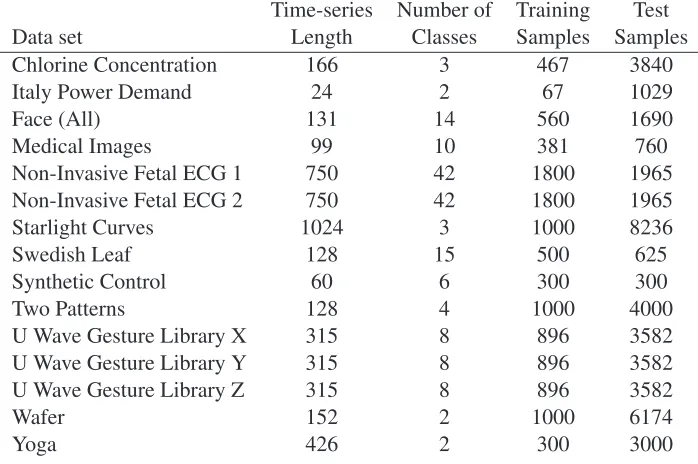
Table 1: Time-series Data Sets
7. Experiments
Section 7.1 details the data sets, experimental set-up, and classifiers used. We first compare the proposed methods to construct setsAof measureτ, reported in Section 7.2, and the proposed esti-mation methods for the moments ofPX|z, reported in Section 7.3. Then in Section 7.4, we show that
applying a dimensionality reduction method can greatly reduce the computation needed at test time. Lastly, we compare our recommended reliable classifier to other approaches to early classification.
Research-grade code and the experimental data sets are available to download.2 7.1 Experimental Set-up and Details
We demonstrate performance using all of the time-series data sets available on theUCR Time-Series Classification and Clustering Page(Keogh et al., 2006) that have at least five hundred test samples and at least 15 training examples per class when this paper was written. We use the given training and test splits, so all results can be reproduced. We also use the Synthetic Control data set from this repository, a data set of Gaussian data that has only three hundred test samples, to further illustrate the differences between the constraint sets and estimation methods that we have described for the proposed incomplete decision rule. Table 1 gives details for the used data sets.
The time-series classification experiments are performed as follows. The test data set consists ofnsampled time-series vectors and corresponding labels{xi,gi}ni=1, withxi∈Rd andg∈
G
. Attimet, the incomplete data for the ith test time-series iszi∈Rt, the firstt samples ofxi. At each
timet we check the proposed incomplete decision rule and classifyziif the reliability condition is
met forτ. We plot results for a set of choices ofτ.
Local QDA Linear SVM
Chebyshev Quadratic Box Chebyshev Quadratic Box
Synthetic Control 1.8 0.7 0.4 0.4 0.3 0.3
Medical Images 27.1 2.7 1.4 1.9 1.0 0.8
Two Patterns 12.45 2.0 1.0 1.8 0.5 0.3
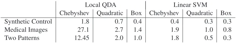
Table 2: Average test time per sample, in seconds, for the three different constraint sets.
Let ti(τ) be the minimum time at which the ith test signal can be classified with reliability
constraint τ, and let ˆg(zi(τ)) be the class label assigned to zi at this time. We measure the test
reliability as 1n∑ni=1I(gˆ(zi(τ)) =gˆ(xi)), where ˆg(xi)is the label assigned to the complete data and
I(·)is one if the argument is true and zero otherwise. We also measure the average classification time as the mean of theti(τ). Ideally, we would like to classify with the smallest average classification
time while still meeting reliability requirementτ.
We perform incomplete classification experiments with two different discriminant classifiers. The first classifier is local QDA (Garcia et al., 2010). Local QDA learns the mean and covariance for the classgdiscriminant function for test pointx, fg(x), by estimating them using thek nearest
classgtraining points to test pointx. We choosek∈ {1, 2, 4, 8, 16, 32, 64, 128}by cross-validation on the training data. In our implementation of local QDA, we use a diagonal covariance matrix, and we regularize the covariance estimate by adding 10−4I, where I is the identity matrix. Since we do not have the complete datax, we instead estimate the mean and covariance for fg(x)by finding the
nearest classgneighbors to the mean ofX. The second classifier that we use is a linear SVM which we implement using LibSVM (Chang and Lin, 2011) with default settings.
7.2 Comparison of Construction of Sets of Measureτ
We first compare the three set construction methods proposed Section 3, the Chebyshev set (3), the Gaussian n¨aive Bayes quadratic set (4), and the Gaussian n¨aive Bayes box set (5).
We vary the reliability parameter between four valuesτ= [0.001, 0.1, 0.25, 0.9], and we perform prediction using the jointly Gaussian model (16). Figure 6 plots the results for the Synthetic Control, Medical Images, and Two Patterns data sets. In all cases, the empirical reliability rate exceeds the reliability requirement τ. Additionally, these plots verify that the Chebyshev set is the most conservative, as it waits the longest to classify the test data, and the n¨aive Bayes quadratic set is the least conservative.
Table 2 compares the average testing time per test sample for the three different constraint sets whenτ=0.9. This table shows that the n¨aive Bayes box set is the least computationally complex, followed by the n¨aive Bayes quadratic set, and finally the Chebyshev set.
7.3 Comparison of Estimation Methods
In this section we compare the performance of reliable incomplete classification using jointly Gaus-sian estimation (16) to that using GMM estimation (17). We use the same classifiers and values for τas given in the previous section.
Gaus-Synthetic Control (local QDA) Synthetic Control (SVM)
35 40 45 50 55
97.5 98 98.5 99 99.5 100
Average Classification Time
Test Reliability Chebyshev
Naive Bayes Quadratic Naive Bayes Box
τ = 0.9
45 50 55 60
90 92 94 96 98 100
Average Classification Time
Test Reliability Chebyshev
Naive Bayes Quadratic Naive Bayes Box
τ=0.9
Medical Images (local QDA) Medical Images (SVM)
60 70 80 90 100
92 94 96 98 100
Average Classification Time
Test Reliability Chebyshev
Naive Bayes Quadratic Naive Bayes Box
τ = 0.9
85 90 95 100
92 94 96 98 100
Average Classification Time
Test Reliability Chebyshev
Naive Bayes Quadratic Naive Bayes Box
τ=0.9
Two Patterns (local QDA) Two Patterns (SVM)
100 105 110 115 120 125
95 96 97 98 99 100
Average Classification Time
Test Reliability Chebyshev
Naive Bayes Quadratic Naive Bayes Box
τ = 0.9
116 118 120 122 124 126
90 92 94 96 98 100
Average Classification Time
Test Reliability Chebyshev
Naive Bayes Quadratic Naive Bayes Box
τ=0.9
Synthetic Control (local QDA) Synthetic Control (SVM)
20 30 40 50
96 97 98 99 100
Average Classification Time
Test Reliability
Joint Gaussian GMM
τ = 0.9
35 40 45 50 55 60
90 92 94 96 98 100
Average Classification Time
Test Reliability
Joint Gaussian GMM
τ=0.9
Medical Images (local QDA) Medical Images (SVM)
55 60 65 70 75 80
90 92 94 96 98
Average Classification Time
Test Reliability
Joint Gaussian GMM
τ = 0.9
80 85 90 95 100
92 94 96 98 100
Average Classification Time
Test Reliability
Joint Gaussian GMM
τ=0.9
Two Patterns (local QDA) Two Patterns (SVM)
100 105 110 115
92 94 96 98 100
Average Classification Time
Test Reliability
Joint Gaussian GMM
τ = 0.9
114 116 118 120 122 124
88 90 92 94 96 98 100
Average Classification Time
Test Reliability
Joint Gaussian GMM
τ=0.9
Local QDA Linear SVM Joint Gaussian GMM Joint Gaussian GMM
Synthetic Control 0.7 0.9 0.3 0.7
Medical Images 2.7 5.5 1.0 2.7
Two Patterns 2.0 3.4 0.5 0.8
Table 3: Average test time per sample, in seconds, for the two different estimation methods.
sian over allτvalues for both classifiers. On the Two Patterns data set with local QDA classification, the GMM method is not uniformly better than the jointly Gaussian method.
Table 3 compares the total testing time of the two approaches, and as expected, the GMM method requires more test time than the simpler jointly Gaussian method.
7.4 Dimensionality Reduction Features
An advantage of our reliable incomplete classification approach is that it can use any features derived from the data for which we can estimate the mean and covariance. As an example alternative to using the time-series samples as the features, we select a smaller feature set by first preprocessing the time-series using supervised linear dimensionality reduction. Linear dimensionality reduction finds a matrixB∈Rℓ×d, ℓ <d that maps the data fromd-dimensional toℓ-dimensional space. Supervised dimensionality reduction uses the label information in the training data to find a reduced space where the data is also separated by class. In the context of incomplete data classification, the complete data becomes the vectorBx∈Rℓas opposed tox∈Rd.
Linear dimensionality reduction can provide two advantages over classifying the time-series features. First, it can diminish the impact of noisy or non-discriminative features in the time-series data, thus providing increased accuracy. Second, reducing the number of features reduces the com-putational complexity. For a time-series withd samples, there ared−tunknown samples at time
t. Thus, if we simply use the time-series samples as the features for classification, the optimization problem that the reliable incomplete classifier must solve hasd−tfree variables. For a long time series, this can cause the computational complexity to become extreme whent is small. However, performing linear dimensionality reduction reduces the number of unknowns toℓwhich can greatly reduce the number of variables in the optimization for reliable classification.
Time-series Number of Test time LDG test time Data set length LDG features at t=1 (ms) at t=1 (ms)
Chlorine Concentration 166 42 76 4
Italy Power Demand 24 2 2 1
Face (All) 131 30 40 2
Medical Images 99 11 18 2
Non-Invasive Fetal ECG 1 750 30 6,107 4
Non-Invasive Fetal ECG 2 750 23 5,789 3
Starlight Curves 1024 26 15,697 2
Swedish Leaf 128 20 35 2
Synthetic Control 60 7 9 1
Two Patterns 128 22 31 2
U Wave Gesture Library X 315 12 418 2
U Wave Gesture Library Y 315 6 382 1
U Wave Gesture Library Z 315 10 393 2
Wafer 152 17 55 2
Yoga 426 26 945 2
Table 4: Time-series length and the number of features after LDG dimensionality reduction as well as a comparison of the testing time, in milliseconds, required to perform reliable local QDA classification with the n¨aive Bayes quadratic constraint set and jointly Gaussian es-timation. The test time shown measures the average time, per test sample, to perform reliable classification at timet=1. Therefore, this is a worst case test time in terms of real-time performance as the number of unknowns in the optimization problem for reliable classification is maximized at timet=1.
7.5 Comparison to Other Methods
Chlorine Concentration Italy Power Demand
100 110 120 130 140 150 160 170 80
85 90 95 100
Average classification time
Test Reliability
Rel. Class. LDG Rel. Class. ECTS
Fixed−time QDA Fixed−time 1−NN
0 5 10 15 20 25
60 70 80 90 100
Average classification time
Test Reliability
Rel. Class. LDG Rel. Class. ECTS
Fixed−time QDA Fixed−time 1−NN
Face (All) Medical Images
100 110 120 130 140 80
85 90 95 100
Average classification time
Test Reliability
Rel. Class. LDG Rel. Class. ECTS
Fixed−time QDA Fixed−time 1−NN
65 70 75 80 85 90 95 100 75 80 85 90 95 100
Average classification time
Test Reliability
Rel. Class. LDG Rel. Class. ECTS
Fixed−time QDA Fixed−time 1−NN
Non-invasive Fetal ECG 1 Non-invasive Fetal ECG 2
620 640 660 680 700 720 740 80
85 90 95 100
Average classification time
Test Reliability
LDG Rel. Class. ECTS
Fixed−time QDA Fixed−time 1−NN
600 650 700 750
85 90 95 100
Average classification time
Test Reliability
LDG Rel. Class. ECTS
Fixed−time QDA Fixed−time 1−NN
Starlight Curves Swedish Leaf
800 850 900 950 1000 1050 92
94 96 98 100
Average classification time
Test Reliability
LDG Rel. Class. ECTS
Fixed−time QDA Fixed−time 1−NN
80 90 100 110 120 130 75 80 85 90 95 100
Average classification time
Test Reliability
Rel. Class. LDG Rel. Class. ECTS
Fixed−time QDA Fixed−time 1−NN
Two Patterns U Wave Gesture Library X
100 105 110 115 120 125 130 70
80 90 100
Average classification time
Test Reliability
Rel. Class. LDG Rel. Class. ECTS
Fixed−time QDA Fixed−time 1−NN
200 220 240 260 280 300 320 75 80 85 90 95 100
Average classification time
Test Reliability
Rel. Class. LDG Rel. Class. ECTS
Fixed−time QDA Fixed−time 1−NN
U Wave Gesture Library Y U Wave Gesture Library Z
150 200 250 300
60 70 80 90 100
Average classification time
Test Reliability
Rel. Class. LDG Rel. Class. ECTS
Fixed−time QDA Fixed−time 1−NN
200 220 240 260 280 300 320 70
80 90 100
Average classification time
Test Reliability
Rel. Class. LDG Rel. Class. ECTS
Fixed−time QDA Fixed−time 1−NN
Wafer Yoga
40 60 80 100 120 140 94
96 98 100
Average classification time
Test Reliability
Rel. Class. LDG Rel. Class. ECTS
Fixed−time QDA Fixed−time 1−NN
300 320 340 360 380 400 420 90 92 94 96 98 100
Average classification time
Test Reliability
LDG Rel. Class. ECTS
Fixed−time QDA Fixed−time 1−NN
Figure 9: Average classification time vs test reliability for reliable incomplete local QDA classifica-tion (Rel. Class.), reliable incomplete local QDA classificaclassifica-tion with LDG features (LDG Rel. Class.), ECTS, Fixed-time local QDA, and Fixed-time 1-NN.
We also compare to the performance of two baseline methods that we callFixed-time local QDA
andFixed-time 1-NN. These methods use no predictive power, but instead classify all test signals at some user specified time:tsamples.
Chlorine Concentration Italy Power Demand
100 120 140 160
50 60 70 80
Average classification time
Test Accuracy
Rel. Class. LDG Rel. Class. ECTS
Fixed−time QDA Fixed−time 1−NN
0 5 10 15 20 25
60 70 80 90 100
Average classification time
Test Accuracy
Rel. Class. LDG Rel. Class. ECTS
Fixed−time QDA Fixed−time 1−NN
Face (All) Medical Images
100 110 120 130 140
50 55 60 65 70 75
Average classification time
Test Accuracy
Rel. Class. LDG Rel. Class. ECTS
Fixed−time QDA Fixed−time 1−NN
70 80 90 100
60 65 70
Average classification time
Test Accuracy
Rel. Class. LDG Rel. Class. ECTS
Fixed−time QDA Fixed−time 1−NN
Non-invasive Fetal ECG 1 Non-invasive Fetal ECG 2
650 700 750
60 70
80 90
Average classification time
Test Accuracy
LDG Rel. Class. ECTS
Fixed−time QDA Fixed−time 1−NN
600 650 700 750
75
80 85 90
Average classification time
Test Accuracy
LDG Rel. Class. ECTS
Fixed−time QDA Fixed−time 1−NN
Starlight Curves Swedish Leaf
750 800 850 900 950 1000 1050
70 80 90
Average classification time
Test Accuracy
LDG Rel. Class. ECTS
Fixed−time QDA Fixed−time 1−NN
80 90 100 110 120 130
60 70 80 90
Average classification time
Test Accuracy
Rel. Class. LDG Rel. Class. ECTS
Fixed−time QDA Fixed−time 1−NN
Two Patterns U Wave Gesture Library X
100 110 120 130
60 70 80 90 100
Average classification time
Test Accuracy
Rel. Class. LDG Rel. Class. ECTS
Fixed−time QDA Fixed−time 1−NN
200 220 240 260 280 300 320
60 65 70 75 80
Average classification time
Test Accuracy
Rel. Class. LDG Rel. Class. ECTS
Fixed−time QDA Fixed−time 1−NN
U Wave Gesture Library Y U Wave Gesture Library Z
150 200 250 300 350
50 55 60 65 70
Average classification time
Test Accuracy
Rel. Class. LDG Rel. Class. ECTS
Fixed−time QDA Fixed−time 1−NN
200 220 240 260 280 300 320
50 55 60 65 70
Average classification time
Test Accuracy
Rel. Class. LDG Rel. Class. ECTS
Fixed−time QDA Fixed−time 1−NN
Wafer Yoga
50 100 150
90 95 100
Average classification time
Test Accuracy
Rel. Class. LDG Rel. Class. ECTS
Fixed−time QDA Fixed−time 1−NN
300 350 400
78 80 82 84
Average classification time
Test Accuracy
Rel. Class. LDG Rel. Class. ECTS
Fixed−time QDA Fixed−time 1−NN
Figure 11: Average classification time vs test accuracy for reliable incomplete local QDA classi-fication (Rel. Class.), reliable incomplete local QDA classiclassi-fication with LDG features (LDG Rel. Class.), ECTS, Fixed-time local QDA, and Fixed-time 1-NN.
run time. However, reliable classification with LDG features performs well on these data sets and is fast, as shown in Table 4.
Finally, Figures 10 and 11 plot the test accuracy of the various approaches. The accuracy plots show that local QDA achieves higher accuracy than 1-NN on most of the data sets; therefore, ECTS suffers in comparison to reliable local QDA due to the fact that it attempts to match a less accurate classifier.
The accuracy plots also show that although ECTS is typically more reliable than fixed-time 1-NN, it is less accurate for at least one value of MS on twelve of the fourteen data sets. On the other hand, reliable local QDA using the time-series samples as features is less accurate than fixed-time local QDA on only the Medical Images and Chlorine Concentration data sets. However, on the Chlorine Concentration data sets, reliable local QDA with LDG features greatly exceeds the accuracy of fixed-time local QDA. Furthermore, although it is not shown in the figure, reliable local QDA classification using GMM based estimation exceeds the accuracy of fixed-time local QDA on the Medical Images data set. In fact, the proposed reliable classification approach can be used with a wide variety of features, classifiers, and estimation methods in order to maximize accuracy for a particular application.
8. Discussion and Some Open Questions
We have proposed a practical incomplete decision rule that is a conservative approximation of the optimal rule. Experiments on a set of time-series data showed consistently earlier and more reliable predictions on average than other approaches. We showed that for linear or quadratic classifiers the proposed decision rule can be checked either with an analytic solution or using convex optimization. We only touched on applying the proposed rule to nearest neighbor classifiers, and it is an open question how to apply this approach efficiently to other classification strategies. In particular, we suspect the proposed approach could also be implemented efficiently with decision trees that use a cascade of linear discriminants.
This paper has focused on answering the question “With probability τ, will the classification decision from this incomplete data be the same as from the complete data?” The presented tools can also be used to answer the related question: “If we classify based on the current incomplete data, what is the probability that assigned label will match that which would be chosen using the complete data?” The answer can be computed by finding the largestτthat makes the first question a “Yes,” which may require guessing aτ, solving the first question, refiningτup or down depending on the answer, and iterating.
Another related question that can be answered is, “Can we reliably classify as classgwith this incomplete data?” That is, there may be only one class (or a subset of classes) which we would like to identify with incomplete data. For example, in determining if a cyst is cancerous or benign, doctors will often have a patient come back every few months to see how it changes over time. There is generally no rush to call it benign, but one would like to classify it as cancerous as soon as that is a reliable class label. This question can be answered by applying the incomplete decision rule given in (2) only to the class of interest.
Acknowledgments
a multi-program laboratory managed and operated by Sandia Corporation, a wholly owned sub-sidiary of Lockheed Martin Corporation, for the U.S. Department of Energy National Nuclear Se-curity Administration under contract DE-AC04-94AL85000. We thank Bela A. Frigyik for helpful discussions.
Appendix A. Proofs
Proof of Proposition 1: For the minimum problem (9), the Lagrange dual function is g(λ) =
βTm− 1
4λBTRB+b−λδ, a concave function of λ, and g(λ) is maximized for λ∗ = q
1 4δBTRB.
Sinceλ∗≥0, it is dual feasible. Since the objective function is convex, strong duality holds, and thus the maximum of the dual problem equals the minimum of the primal problem. A similar analysis can be performed for the maximum problem.
Proof of Proposition 2:First, note that each pairwise check reduces the number of classes labelled candidateby either two classes if the classes tie, or by one class (the loser) if one class dominates. Second, once a class has tied with another class or has been dominated, it cannot be the correct dominating class. Thus the proposed decision process eventually reduces the number of classes labelledcandidateto either zero or one. If there are zero classes left labelledcandidate, then all classes have either tied or been dominated, and the above process correctly chooses not to classify. If there is one class remaining that is labelledcandidateit must be compared to all the classes that tied on their first comparison. It is not necessary to also compare to the classes labelleddominated by the transitivity of the domination rule.
Proof of Proposition 3: We first note that in theComparestep, the pairwise comparison between classescandhrequires a single minimum computation ifcdominatesh, and two computations if the classes tie or ifhdominatesc. Furthermore, we defineT to be the number of pairwise comparisons that result in ties during the Compare step, and D as the number of pairwise comparisons that do not result in a tie in the Compare step (such evaluations necessarily result in one class that was labelled candidatebeing re-labelled dominated). Thus, the compare step requires at most 2T+2Dminimum calculations.
On the other hand, each pairwise comparison in the Final Comparison check requires only a single minimum computation.
There are two cases to consider
Case 1: Consider the case that the Compare step in the decision process results in one class left labelledcandidate. Immediately prior to theFinal Comparisonstep, there areG−1 classes that have been re-labelledtiedordominated, and since each tie results in two classes being re-labelled tied, it must be that
G−1=D+2T. (19)
In theFinal Comparisonstep, theGth class must be compared to at most the 2T classes labelled tied, each of which requires one minimum calculation. Thus the maximum number of calculations needed is
2T+2D+2T =2(G−1)by (19).
Case 2: The second case is that at the end of theCompare step there are zero classes labelled candidate. Therefore,
G=D+2T, (20)
and the total number of comparisons required is
2T+2D=G+Dby (20).
There can be at most G−2 comparisons that result in one class dominating the other (otherwise, one class would remain labelledcandidateafter theComparestep), so the maximum number of minimum calculations is again 2(G−1).
Since it requires at least one minimum calculation change a class label from candidate to dominatedortied, the minimum number of calculations isG.
Appendix B. Gradient Descent Solution for the Quadratic Min and Max Problems
The min problem with quadratic f(x)subject to a quadratic constraint set is written as min
x∈A f(x) =minx (x−v)
TV(x−v) +b (21)
s.t.(x−m)R−1(x−m)≤δ,
whereV is indefinite andRis positive semi-definite. We propose to solve this problem using the two-step gradient descent approach described in Tao and An (1997).
We first reformulate (21) as thetrust region subproblem(TRSP). Define
z=R−21(x−m),
A=2R12V R12,
y=2R12V(m−v),
btsr p=b+vTV v+mTV m−2mTV v.
Then rewrite (21) as
min
x∈A f(x) =minz
1 2z
TAz+yTz+b
tsr p (22)
s.t. kzk≤√δ.
Letρequal the largest eigenvalue ofA. The following two-step iteration converges to az∗that is a local minimum of the TRSP (22):
Step 1 : zk+1=zk−
1
ρ(Azk+y),
Step 2 : zk+1=min
zk+1, k
zk+1k
√
δ zk+1
,
The TRSP has been shown to have at most one local minimum that is not also the global mini-mum (Martinez, 1994), and thus the above algorithm has proven to be robust in finding the minimini-mum of (22).
Furthermore, for the incomplete data decision rule (7), it is not necessary to find the true mini-mum overAof f(x), but it is instead sufficient to know only whether or not it is less than or equal to zero. Therefore, the iteration can be stopped early ifzTkAzk+yTzk+btsr p≤0.
Appendix C. Derivation of the Variance for GMM Based Estimation
Letmg=E[X|g,z],Rg=COV[X|g,z], andp(g|z)be defined as in Section 5.2.
R= Z
x
(x−m)(x−m)T p(x|z)dx
= Z
xg
∑
∈G(x−m)(x−m)T p(x,g|z)dx
=
∑
g∈G p(g|z)
Z
x
(x−m)(x−m)T p(x|g,z)dx
=
∑
g∈G p(g|z)
Z
x
xxT−2x
∑
h∈GmThp(h|z) +
∑
q∈Gh∑
∈GmqmThp(q|z)p(h|z) !
p(x|g,z)dx
=
∑
g∈G p(g|z)
Z
x
xxT−2xmTg+mgmTg p(x|g,z)dx+
Z
x
2xmTg−2x
∑
h∈GmThp(h|z)p(x|g,z)dx
−mgmTg+
∑
q∈Gh
∑
∈GmqmThp(q|z)p(h|z) !
=
∑
g∈G
p(g|z) Rg+2mgmTg−2mg
∑
h∈GmThp(h|z)−mgmTg+
∑
q∈Gh∑
∈GmqmThp(q|z)p(h|z) !
=
∑
g∈G
p(g|z) Rg+mgmTg−2mg
∑
h∈GmThp(h|z)
!
+
∑
q∈Gh
∑
∈GmqmThp(q|z)p(h|z)
=
∑
g∈G
p(g|z) Rg+mgmTg
−
∑
q∈Gh
∑
∈GmqmThp(q|z)p(h|z).
References
H. S. Anderson, N. Parrish, K. Tsukida, and M. R. Gupta. Reliable early classification of time series. InICASSP, 2012.
P. Armitage. Sequential Analysis with More than Two Alternative Hypotheses, and its Relation to Discriminant Function Analysis. Journal of the Royal Statistical Society. Series B (Methodologi-cal), 12(1):137–144, January 1950.
C.-C. Chang and C.-J. Lin. LIBSVM: A library for support vector machines.ACM Trans. Intelligent Systems and Technology, 2:27:1–27:27, 2011. Software available athttp://www.csie.ntu. edu.tw/˜cjlin/libsvm.
M. Cooke, P. Green, L. Josifovski, and A. Vizinho. Robust automatic speech recognition with missing and unreliable acoustic data. Speech Communication, 34(3):267 – 285, 2001.
M. C. Costanza and A. A. Afifi. Comparison of Stopping Rules in Forward Stepwise Discriminant Analysis. Journal of the American Statistical Association, 74(368):777–785, January 1979. K. Crammer and Y. Singer. Ultraconservative online algorithms for multiclass problems. Journal
Machine Learning Research, 3:951–991, 2003.
M. Dredze, K. Crammer, and F. Pereira. Confidence-weighted linear classification. Intl. Conf. Machine Learning (ICML), 2008.
T. Ferguson. Optimal Stopping Rules and Applications. E-book available on the author’s website., 2001.
J. Friedman, R. Kohavi, and Y. Yun. Lazy decision trees. InProc. AAAI, 1996.
W. J. Fu, E. R. Dougherty, B. Mallick, and R. J. Carroll. How many samples are needed to build a classifier: a general sequential approach. Bioinformatics, 21(1):63–70, January 2005.
E. K. Garcia, S. Feldman, M. R. Gupta, and S. Srivastava. Completely lazy learning. IEEE Trans. Knowledge and Data Engineering, 22(9):1274–1285, Sept. 2010.
T. Hastie, R. Tibshirani, and J. Friedman. The Elements of Statistical Learning. Springer-Verlag, New York, 2001.
E. Keogh, X. Xi, L. Wei, and C. A. Ratanamahatana. The UCR time series classification and clustering webpage. 2006.
J. M. Martinez. Local minimizers of quadratic functions on Euclidean balls and spheres. SIAM J. Optimization, 4(1):159 – 176, 1994.
S. Pang, S. Ozawa, and N. Kasabov. Incremental linear discriminant analysis for classification of data streams. IEEE Trans. Systems, Man, and Cybernetics, 35(5):905–914, October 2005. N. Parrish and M. R. Gupta. Dimensionality reduction by local discriminative Gaussians. InProc.
Intl. Conf. on Machine Learning (ICML), 2012.
B. Raj and R.M. Stern. Missing-feature approaches in speech recognition. Signal Processing Mag-azine, IEEE, 22(5):101 – 116, 2005.
B. Raj, M. L. Seltzer, and R. M. Stern. Reconstruction of missing features for robust speech recog-nition. Speech Communication, 43(4):275 – 296, 2004.
A. Rogier, T. Donders, Geert J. M. G. van der Heijden, T. Stijnen, and K. G. M. Moons. Review: A gentle introduction to imputation of missing values. J. of Clinical Epidemiology, 59(10):1087– 1091, 2006.
M. Saar-Tsechansky and F. Provost. Handling missing values when applying classification models.
Journal Machine Learning Research, 2007.
J. L. Schafer and J. W. Graham. Missing data: Our view of the state of the art. Psychological Methods, 7(2):147–177, 2002.
D. Schuurmans and R. Greiner. Learning to classify incomplete examples. InComputational Learn-ing Theory and Natural LearnLearn-ing Systems: MakLearn-ing LearnLearn-ing Systems Practical, 2007.
P. D. Tao and L. T. H. An. Convex analysis approach to D.C. programming: theory, algorithms, and applications. ACTA Mathematica Vietnamica, 22(1):289 – 355, 1997.
A. Wald. Sequential Analysis. John Wiley, 1947.

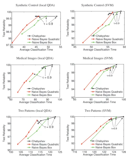
![Figure 7: Average classification time vs test reliability for local QDA (left column) and linearSVM (right column) using the n¨aive Bayes quadratic constraint set with τ varied between[0.001, 0.1, 0.25, 0.9].](https://thumb-us.123doks.com/thumbv2/123dok_us/9816449.1967494/17.612.90.524.101.626/figure-average-classication-reliability-linearsvm-quadratic-constraint-varied.webp)