A Case Study on Meta-Generalising: A Gaussian Processes Approach
Grigorios Skolidis [email protected]
Guido Sanguinetti [email protected]
School of Informatics University of Edinburgh Edinburgh, EH8 9AB, UK
Editors: S¨oren Sonnenburg, Francis Bach and Cheng Soon Ong
Abstract
We propose a novel model for meta-generalisation, that is, performing prediction on novel tasks based on information from multiple different but related tasks. The model is based on two cou-pled Gaussian processes with structured covariance function; one model performs predictions by learning a constrained covariance function encapsulating the relations between the various training tasks, while the second model determines the similarity of new tasks to previously seen tasks. We demonstrate empirically on several real and synthetic data sets both the strengths of the approach and its limitations due to the distributional assumptions underpinning it.
Keywords: transfer learning, meta-generalising, multi-task learning, Gaussian processes, mixture
of experts
1. Introduction
self-taught learning (Raina et al., 2007) is a setting where labeled data are available for the target task, but the learning algorithm wishes to also use unlabelled data from a source task to improve performance. In its own right, self-taught learning is distinguishable from semi-supervised learning (Chapelle et al., 2006), where labelled and unlabelled data are assumed to come from the same task. The purpose of all these TL approaches is to enhance the generalisation power of a specific algorithm by leveraging related (but different) knowledge from multiple tasks. In particular, it is generally assumed that at least the input data for the target task will be available during the learning, so that a measure of similarity between the training and target tasks can be estimated.
The question that we wish to raise in this work is whether the notion of generalisation can be extended to the level of tasks as a form of meta-generalisation. Meta-generalisation is a concept introduced in Baxter (2000), where the author argues whether a transfer learning algorithm can gen-eralise well on totally unseen tasks after seeing sufficiently many source (or training) tasks. We emphasize that this is much more than a theoretically interesting question. Our motivating example is a strongly applied one: we wish to create an automated diagnosis tool that can accommodate variability among patients, so that, once trained on a sufficient number of patients, it can gener-alise to new patients. In his work Baxter (2000) derives bounds on the generalisation error of this problem in terms of a generalised VC-dimension parameter, as well as comments that the number of source tasks and examples per task required to ensure good performance on novel tasks has to be sufficiently large. While Baxter (2000) derives an algorithm to select a subset of features to perform multi-task learning based on Neural Networks (NN), his work is more on the theoretical side as no experimental results are presented. Besides that, the model proposed in this work needs to be retrained in case a new target task arrives in order to learn a small number of task dependent parameters.
One way to approach meta-generalising is through domain adaptation, by training a model on the data of the source and the target set of tasks (Ben-David et al., 2007). This type of approach, as well as the model proposed in Baxter (2000), are essentially trained in a transductive way, as the algorithm is able to make predictions only on the test tasks that is trained on, or needs to be re-trained in case a new task arrives. Obviously, the performance and the success of domain adaptation algorithms depends strongly on certain assumptions, with most important the similarity between the target and the source distribution (Ben-David et al., 2010). Clearly, if these assumptions are violated then the success of these algorithms is doubtful.
In this paper we investigate the use of coupled Gaussian process models to address this problem. The model uses a multi-class Gaussian process for assigning probabilistically unseen tasks to source tasks (determining task responsibilities), and then uses a multi-task Gaussian process (Bonilla et al., 2008) to perform prediction in individual tasks. Extensive testing on real and simulated data shows the promise of the model, as well as giving insight on the underlying assumptions.
The rest of the paper is organised as follows: in Section 2 we formally define the meta-generalising problem, emphasizing the main assumptions and highlighting the important special case of fully observed tasks. In Section 3 and 4 we present our model and the inference methodol-ogy used. We present our empirical results in Section 5, and we finish in Section 6 by discussing the merits of our model in the context of the wider literature in transfer learning and meta-generalisation.
2. Meta-generalising
In this section, we formally state the problem of meta-generalising, while we introduce the notation that will be used throughout this paper unless specified otherwise. For simplicity, we concentrate on binary classification problems within each task, while we note that the same formalism applies to regression and multi-class classification problems.
In a meta-generalising scenario the learner is provided with a set of source tasks
T
S ={
T
s 1, . . . ,T
s
M} which are used for training the model; testing is then performed on a set of target
tasks
T
T ={T
1t, . . . ,T
t
H}. Each of the M source tasks will contain a training set of input/ output
pairs(x,y), while data from any of the H target tasks are hidden. For later convenience, we will define the whole training set across tasks as a set of triples Ts={xs
i,y
st i ,y
sx i }N
s
i=1, where xsi ∈Rd is
the input feature vector, ysxi ∈ {−1,+1}are the class labels, and ysti ∈ {1, . . . ,M}is the source task label indicating to which task the input/ output pair pertains, and Ns=∑M
j=1nsj is the total number
of training pairs where nsj is number of data points from the jth source task. Moreover, we will
write Xsj ={xs i j}
nsj
i=1 to denote the total item set of the jth source task, while ysxj ={ysxi j} nsj
i=1 and
ystj ={yst
i j} nsj
i=1will be used to denote all class and task labels from the jthsource task. In the rest of
the paper subscript j will be used to refer to tasks, and subscript i to data points.
Each of the H target tasks
T
tj will consist of a set Xtj ={xti j} ntj
i=1 of input points, where ntj is
number of data points from the jth target task and both types of labels are missing. Likewise, the total number of test points will be denoted by Nt=∑Mj=1ntj. For reasons that will become clear later on, it is further assumed that for each target task data point xtj there is information that it comes from the jthtarget task, but there is no knowledge with which of the source tasks is more similar. Note that each source task training input xsi is assigned two types of labels. This implies supervision in both the levels of the tasks and the data, through yst and ysx respectively; task labels yst indicate from which of the source task a specific data point comes from, as a form of meta-level information, and class labels ysx indicate to which class inside the task the data point belongs to, as a form of
inter-task information.
of the source and the target sets X =Xs∪Xt, with N =Ns+Nt. Hence, the errorλewill be given
by,
λe= N
∑
i=1
|ft(xi)−fs(xi)|,
where xi∈X . Intuitively, if the errorλeis large then there is a disagreement between the labels of the
source and target tasks distribution. Also note that, in a multi-task scenario the parameterλecan be
computed by training two separate models under the same learning framework (e.g., NN, GPs, etc) since labeled data are available for both the source and target task. Thus, the predictive functions of the source and target task can be estimated separately andλe can also be used as an empirical
measure of the relatedness of the two tasks. Conversely, in the scenarios of meta-generalising and domain adaptation one has to assume that the errorλe will be low, since labels are available only
for the source tasks. If one of these assumptions is not valid, then meta-generalisation can not be expected to guarantee success.
We now give a formal definition of meta-generalising.
Definition 1 Given a set of source tasks
T
S and a set of target tasksT
T, meta-generalising is aninductive inference method that aims at making predictions on the set of target tasks by sampling the space of source tasks .
We further define two possible scenarios: in the fully observed tasks case, we assume that the similarity of the distribution assumption is perfectly met, so that the data generating distribution of the target task is the same as that of one of the source tasks (but we do not know which one). This assumption is relaxed in the partially observed tasks scenario, where we still assume similarity of the distribution but we do not necessarily have identity.
The meta-generalising setting implies that there is hierarchical structure in the problem. The data of each task are on the base level and the distribution of the tasks is on the meta level. Hence, it is intuitive that mechanisms are required to
1. Model the distribution of the data of each task, and the distribution of the source tasks (corre-lation between tasks).
2. Infer the level of correlation between the target task and the source tasks.
The first prerequisite leads us to multi-task learning, as many approaches offer mechanisms to model both the data and the task distribution (Bakker and Heskes, 2003; Yu et al., 2005; Ando and Zhang, 2005; Xue et al., 2007; Argyriou et al., 2008; Bonilla et al., 2008; Daum´e III, 2009). Following the multi-task route, informally speaking, the second prerequisite can be translated as the problem of which of the M outputs of the multi-task classifier to select to make predictions for the target task. In some cases, task-descriptor features may be available, giving a direct measure of task similarity. In this work, we are interested in the general case where no reliable task descriptor features are available; we will then learn similarities between tasks through a distribution matching pursuit.
Another way of approaching the problem of meta-generalisation is through the framework of
mixtures of experts (ME) (Jacobs et al., 1991; Waterhouse, 1997), under which a bigger
data generating mechanism of each task; under the ME framework each expert is used to model the data generating process of each subproblem. These experts are then combined through a gating network that models the responsibilities of the experts on each data partition. Hence, attacking the meta-generalisation problem through the ME framework can be seen as an unsupervised alternative method to that problem, that does not use the information about the origins of each task (the source task labels) but instead allows the algorithm to automatically infer the data partitions and the regions of expertise of each expert. Therefore the ME approach is in direct connection to multi-task learning and meta-generalisation in which cases the experts are equivalent to the tasks, and this framework could be used as a rough lower bound on the performance of a multi-task classifier. Note though that in principle it would be desirable to be able to automatically infer the number of experts as in Rasmussen and Ghahramani (2001) which can be seen as a similar mechanism of finding cluster of tasks, in contrast with the method of ME with GPs in Tresp (2000) where the number of experts had to be known a priori.
3. A Model for Meta-generalisation
Having identified the nature of the problem, we now propose a model for meta-generalising. The model builds upon the multi-task learning framework of Bonilla et al. (2008) which is able to capture the dependencies between the data and the tasks. In addition, we employ a classifier over the tasks to learn the task labels (from which task each data point comes from). Both of those two learning mechanisms, multi-task setting and classification of the tasks, are modeled by Gaussian Processes (GPs), which are coupled by sharing a common hyper-prior. In the rest of this section, we first give a short introduction to GPs and we review multi-task learning with GPs of Bonilla et al. (2008), we then present the model for meta-generalising, and finally we describe how to make predictions on new tasks.
3.1 Multi-task Learning with Gaussian Processes
Gaussian processes (Rasmussen and Williams, 2005) provide a flexible modelling framework for supervised learning which has become increasingly popular in recent years. A Gaussian Process is a probability distribution over functions f , where the joint distribution of function evaluations over a finite set of inputs is a multivariate Gaussian distribution. At core of the GP prediction is the
covariance function or kernel, parameterised byθx, that models the output covariance at different pairs of input points, and in essence acts as a measure of similarity between different input locations. In order for a covariance function to be valid it has to be positive semidefinite, and has to satisfy Mercer’s theorem (Rasmussen and Williams, 2005).
In a multi-task scenario the interest lies in learning M related functions fj, j=1, . . . ,M, from training data xi j, yi j, i=1, . . . ,nj, with x∈ R
d, and n
1+. . .+nM=N. In the following of this section, data points from task j will be denoted by Xj= [x1 j, . . . ,xnjj]and X= [X1, . . . ,XM]will be used to denote the set of all data points. Focussing on a regression problem for simplicity, the noise model will be given by
yi j= fj(xi j) +εj, withεj∼
N
(0,σ2
j), (1)
where yi j(xi j) denotes the ithoutput (input) of the jthtask. We note that each input point has M
practice, but function values corresponding to unobserved values can easily be marginalised using the consistency of GPs
The multi-task model of Bonilla et al. (2008), which has been known in the geo-statistics com-munity as the “Intrinsic Model of Coregionalization” (IMC) (Cressie, 1993), can be elegantly re-covered from the theory of matrix variate distributions (Gupta and Nagar, 2000). Define the vector
f by stacking the columns of F= [f1. . .fM]into a single vector, f=vec(F), where fj∈R
N×1is the
column vector of all latent functions evaluations of task j. Then the probability density function of matrix F will be given by:
(2π)−12NM|Kt|− 1 2N|Kx|−
1 2Mexp
−1
2trace
Kt−1F(Kx)−1FT
, (2)
where Kt ∈RM×M and Kx∈RN×N (Gupta and Nagar, 2000). This configuration implies that the matrix Kt models the correlations between the vectors fj, that is, the tasks in the multi-task view,
and Kxmodels the correlations between each element of vectors fj. In the GP framework, this
corre-lation between function evaluations at different input points is captured by the covariance function. Then, by using some matrix algebra involving the vec and Kronecker operator, Equation (2) can be written in the form Bonilla et al. (2008) proposed,
p(f|X) =
GP
(0,Kt⊗Kx).Employing this type of prior for the latent functions f the noise model for the regression problem stated in equation (1) becomes, p(y|f) =
N
(f,D⊗I), where D∈RM×M is diagonal with D
j j=σ2j
and I∈RN×N is the identity matrix.
The key element of this formulation is the task covariance matrix Kt which reflects the task correlations. For example, if Kt was fixed to the identity matrix, then all tasks would be indepen-dent but they would still share the same hyperparameters of the covariance function. Of course, one of the main goals of multi-task learning is to learn these task dependencies. Bonilla et al. (2008) approached this problem by parameterizing the task covariance matrix, with parametersθt, always retaining positive definite restrictions, and treating these parameters as hyperparameters to be learned. Positive definite guarantees were achieved, by parameterizing a lower triangular matrix
L to employ the Cholesky factorization Kt =LLT. Most importantly, parameters related to the data covariance function or the task covariance matrix can be learned in the standard GP formulation, by maximizing the marginal likelihood p(y|X) =R p(y|f)p(f|X)df.
3.2 Model
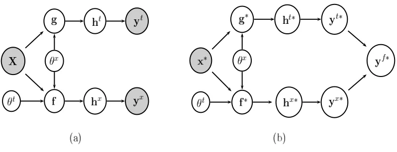
In this section we describe the Coupled Multi-Task Multi-Class (CMTMC) model we propose for meta-generalisation. The objectives of the model are first to model the dependencies between the tasks, and second to assign unseen tasks to source tasks by finding task similarities. The first ob-jective is met through the Multi-task part of the model, while the second is achieved through the Multi-class classifier. Figure 1 shows the graphical model of the CMTMC classifier. In this subsec-tion we use x,yt, and y
x to refer to xs
, y
st
, and y
sx to keep the notation light, since in the learning
phase only source tasks are involved. Therefore, notation introduced in Section 3.1 applies here. Moreover, from Section 2 we have that yt ∈ {1, . . . ,M} and yx ∈ {−1,+1}as the task and class
Figure 1: Coupled Multi-Task Multi-Class (CMTMC) model. Variables f and g are the two sets of GPs for the multi-task and multi-class classifiers respectively, whereas variables hx and
ht denote the auxiliary variables of the two classifiers; (a) graphical representation of the training phase, (b) graphical representation of Meta-generalising.
and Chib (1993), we define two sets of auxiliary variables ht =vec(Ht), and hx=vec(Hx), which as shown later on enables the multinomial and the binary probit model respectively. For later con-venience, we will be using htjand htnto denote the jthcolumn and nthrow of matrix Ht.
Figure 1 shows that there are two directed channels of variables. The upper channel, with variables Ct={g,h
t
,y
t}, is responsible for learning the task labels, thus from which task each data
point comes from, while the lower channel, with variables Cx ={f,h
x
,y
x}, learns to classify the
data points inside every task and to find task correlations, through the standard multi-task classifier. Thus, there are two sets of Gaussian Processes. The first one is responsible for the classification over the tasks g|X,θ
x∼
GP
(0,I⊗Kx), where g=vec(G), G= [g1, . . . ,gM], and gj∈R
N×1. The
second one is responsible for the multi-task classification f|X,θ
x
,θ
t ∼
GP
(0,Kt⊗Kx), where asstated before variables θx andθt are used to denote the hyperparameters of the data covariance function and task matrix respectively. As in the multi-class case we will have that f=vec(F), where
F= [f1, . . . ,fM]and fj ∈R
N×1. In the rest of the paper we will write Kx to denote the covariance
matrix between all data points X, unless specified otherwise. Moreover, I and Kt will be M×M,
where the identity matrix in the multi-class case implies independence between the classes, thus
gj|X,θ
x∼
GP
(0,Kx). The key objective is to learn M functions gjfor the multi-class classifier and M related functions fj for the multi-task classifier.
Note that the data covariance matrix Kx is shared by both sets of processes g and f. This is graphically illustrated by the fact that the node of hyperparameters θx is connected to both latent functions; thus, the multi-class and the multi-task classifier share the same hyperparameter space forθx. The multi-class classifier is restricted to have the same covariance function across the classes
in contrast with the standard model for multi-class classification with GPs, which in principle al-lows you to use different covariance functions across classes. In fact, the CMTMC model could be decoupled into two separate classifiers with different sets of hyperparametersθx between the two
restriction does not affect the performance. In contrast, it reduces dramatically the computational cost since the hyperparameters of the data covariance function need to be estimated only one time.
The probit model is enabled in both channels by a standardized normal noise model over the auxiliary variables, hti j|gi j∼
N
(gi j,1), and hx
i|fi ∼
N
(fi,1)(Albert and Chib, 1993; Csat´o et al., 2000; Girolami and Rogers, 2006; Skolidis and Sanguinetti, 2011). The relationship between out-puts yt and yxand auxiliary variables ht, and hxis deterministic and will be given by:yti= j if htji= max
1≤k≤M{h t ki},
p(yxi|hx i) =
(
δ(hxi)δ(yxi) if yxi = +1
δ(−hx
i)δ(−yxi) if yxi =−1
,
whereδis one if its argument is positive and zero otherwise, which completes the specification of the model.
3.2.1 INFERENCE
Classification problems imply non-Gaussian noise models, which make inference intractable. To address this intractability, we adopt a variational approximate treatment to the problem, as it is computationally more efficient than sampling-based methods while retaining a reasonable accuracy in empirically approximating posterior marginals.1For a comprehensive comparison between these approximations for GP multi-class classification, and on the multinomial probit model the interested reader in referred to Girolami and Rogers (2006). The dependencies of the random variablesΘ= {g,h
t
,f,h
x}are depicted graphically in Figure 1.a and are summarized in the joint likelihood of the
CMTMC model as:
p(yt,y
x
,Θ|θ
x
,θ
t
,X) =p(y
t|ht)p(ht|g)p(g|θx
,X)p(y
x|hx)p(hx|f)p(f|θx
,θ
t
,X).
Variational methods approach this problem by approximating the joint posterior of the latent variablesΘwithin a family of tractable distributions; in our case, we will approximate the joint pos-terior as a factored distribution p(Θ|yt,y
x
,X,θ
t
,θ
x)≈Q(Θ) =∏
i=1Q(Θi) =Q(g)Q(ht)Q(f)Q(hx).
Minimizing the Kullback-Leibler divergence between the approximating and the true distribution is equivalent to maximizing the following lower bound on the marginal likelihood
log p(yt,y
x|X
,θ
x
,θ
t)≥Z Q(Θ)logp(yt,y
x
,Θ|X,θ
x
,θ
t)
Q(Θ) dΘ, (3)
which is found by applying Jensen’s inequality (MacKay, 2003). Standard results show that the distributions that maximize the lower bound are given by
Q(Θi) =
exp(EQ(Θ\Θi){log p(y
t
,y
x
,Θ|X,θ
t
,θ
x)}) R
exp(EQ(Θ\Θi){log p(y
t
,yx,Θ|X,θt,θx)})dΘi
where Q(Θ\Θi)denotes the factorized distribution with the ithcomponent removed. Inference and
learning are performed in a variational EM algorithm: the E-step computes the variational posteri-ors on the variablesΘ, and the M-step optimizes the hyperparametersθt,θ
x given the expectations
computed in the previous step. At each (E or M) iteration the variational lower bound,
L
(Q)(given in Appendix B Equation (15)), provably increases (or at worst remains unchanged), and these two steps are repeated until convergence.2We now briefly summarize the calculations needed to perform the E and M steps. The pseudo-algorithm of the training of the CMTMC model is given in Algo-rithm 3.2.1. We omit any details and emphasize only the occurrence of the special form covariance function we employ; fuller details can be found in Appendices A, and B.E-step. The approximate posteriors for the multi-class classifier will be given by,
Q(g) = M
∏
j=1
Ng
j(˜gj,Σg)
, (4)
Q(ht) = N
∏
n=1
N
ytnht
n(˜gn,I), (5)
whereΣg=I+ (Kx)−1−1=Kx(I+Kx)−1, ˜gj=Σg˜htj, and
N
ytn
ht
n(˜gn,I)denotes an M-dimensional
Gaussian distribution truncated such that jthdimension has the largest value if ytn=j. In the lower channel, the approximate posteriors for the multi-task classifier will be given by,
Q(f) =
Nf
(˜f,Σf), (6)Q(hx) = NM
∏
i=1
˜
fi+yxi
N
f˜i(0,1)Φ(yxi f˜i)
!
, (7)
where ˜f=Σf˜hx, andΣf =Kt⊗Kx(I+Kt⊗Kx)−1 and the tilde notation in the above random variables denotes posterior expectation, that is, ˜t(α) =EQ(α){t(α)}; more details can be found in Appendix A.
M-step. The M-step optimises the lower bound with respect to the hyperparametersθx andθt. This is performed by gradient descent; computation of the gradients of the lower bound given in Equation (3) are somewhat intricate and are given in Appendix B.
Algorithm 1 CMTMC model - Training
1: Inputs : Xsj, y
sx j, y
st
j for j=1, . . . ,M
2: Sample parameters g,h
t
,f,h
xfrom prior
3: Initialise hyper-parametersθx,θ
t
4: repeat
5: E-step
6: Compute Q(g)and Q(ht)for MC-classifier, Equations (4),(5)
7: Compute Q(f)and Q(hx)for MT-classifier, Equations (6),(7)
8: M-step
9: Optimize hyperparametersθx,θ
t, Equations (16), (16)
10: Compute Lower-bound on log-marginal likelihood, Equation (15)
11: until convergence
3.3 Prediction on Novel Tasks
While in the previous section we described how to train the model on training data from the source tasks, we now describe how to perform predictions on unseen target tasks. We adopt a mixture of experts type approach; in these networks, multiple outputs are combined and weighted according to the responsibilities they have on a certain prediction task. In a similar manner, the multi-task classifier of the CMTMC model can be seen as a multi-output predictor, and the classifier over the task labels (multi-class) can be used to infer the responsibilities of the outputs of the multi-task classifier, since it produces posterior probabilities of task memberships. Then predictions on novel tasks are computed according to
p(yf∗= +1|x∗,X,y
t
,y
x) =
∑
Mj=1
p(yx∗j = +1|x∗,y
t∗
,X,y
x)p(yt∗
j |x∗,X,y
t)
, (8)
where p(yx∗j = +1|x∗,y
t∗
,X,y
x) =p(yx∗
j = +1|x∗,X,y
x)is the posterior of the jthtask belonging to
class “+1” from the multi-task classifier, and p(ytj∗|x∗,X,y
t)is the posterior of x∗coming from the
jthtask, or the test point task responsibility from the multi-class classifier. A graphical representa-tion of this process is given in Figure 1.b, where it is shown that nodes yt∗, and yx∗are combined to give the final predictions yf∗.
However, the meta-generalisation scenario presents some additional challenges which are not found in classical mixture of experts models. In many cases, a target task consists of a batch of input points, and the simple fact that they all come from the same task contains valuable information about the correlations between the associated outputs. Another closely related issue is that of the correlation between the target task and the source tasks. In many multi-task problems it is a usual phenomenon to observe groups of highly correlated tasks (e.g., Figure 3.b), while other times tasks are correlated but in a more random fashion (e.g., Figure 6.b, 7.b). As we will see in the experimental sections, this can have important consequences in terms of predictive accuracy, and in terms of choosing an appropriate prediction model.
In the following, we present two distinct scenarios for inferring the task responsibilities. Given a target task with nt data points xt∗={xt∗
1,x
t∗ 2, . . . ,x
t∗
nt}, in the first scenario we treat each data point
from the target task individually to infer its task responsibilities, which we will refer to as Point
to Point Gating (P2PGat). This approach neglects the information that all target points come from
the same task, and as we will see in the experimental section, is more appropriate when inter-task correlations are weaker. In the second scenario we wish to combine the information from all nt test points to infer the overall task responsibilities for the target task, which we will refer to as Batch predictions.
3.3.1 POINT TOPOINTGATING
probabilities of the M outputs p(yx∗j = +1|x∗
,X,y
x)of the multi-task classifier, as
p(yx∗j = +1|x∗,X,y
x) =Z p(yx∗
j =1|hx∗)p(hx∗|x∗,X,y
x)dhx∗
,
≡ Z +∞
0
N
hx∗
j (λ
∗ j,υ
∗ j 2
)dhx∗=Φ λ ∗ j υ∗ j ! (9)
where we have used thatυ∗j2=1+kt
j jkxx∗x∗−
kt
j⊗kxx,x∗
T
(I+Kt⊗Kx)−1kt j⊗kxx,x∗
, andλ∗j=
ktj⊗kxx
,x∗(I+K
t⊗Kx)−1˜hx. Additionally, kt j, k
t
j j are used to denote the jth column and the j jth
element of Kt respectively, kxx
,x∗ is used to denote the covariance vector between X and x
∗, andΦis
the probit function.
The second set of quantities are the task responsibilities which are computed from Girolami and Rogers (2006)
p(yt∗=k|x∗,X,y
t) =Z p(yt∗=k|ht∗)p(ht∗|x∗
,X,y
t)dht∗
≡ Z +∞
−∞
N
ht∗
k(µ
∗ k,ν
∗
k)
∏
m6=k Z ht∗
k
−∞
N
ht∗
m(µ
∗ m,ν
∗
m)dht∗mdht∗k, (10)
which can be evaluated using numerical integration as:
p(yt∗=k|x∗,X,y
t) =E p(u)
(
∏
j6=k Φ ν1∗
j
uν∗k+µ∗k−µ∗j !)
, (11)
where u∼
N
u(0,1),ν∗m=1+kxx∗,x∗−k
xT
x,x∗(I+K
x)−1kx
x,x∗, and µ
∗ m=kx
T
x,x∗(I+K
x)−1˜ht m.
In the P2PGat scenario, the novel input points are not assumed to share a common task la-bel. Therefore, class prediction is performed straightforwardly on every new input by inserting the posterior probabilities obtained in Equations (9,10) in the gating network given by Equation (8).
3.3.2 BATCH
In a Bayesian way using all test points xt∗ to infer the overall task responsibility is performed by replacing the univariate distributions from Equation (10) with the appropriate multivariate. As a result the second integral of Equation (10) becomes the multivariate cumulative distribution function
Rht∗
k
−∞
Nh
t∗m(M
g∗ m,Υ
∗)dht∗
m. Specifically the mean and the variance of the auxiliary variables ht∗mon the
batch of test points x∗will be given by:
Mg∗m =E[hmt∗|x∗] =KxxT
,x∗ I+K
x x,x
−1
˜ht
m (12)
Υ∗=cov[ht∗m|x∗] =I+Kxx∗
,x∗−K
xT
x,x∗ I+K
x x,x
−1
Kxx
,x∗, (13)
where KxxT
,x∗ is the N×n
t covariance matrix of all training points X, and all test task data points x∗,
and Kx x∗
,x∗is the n
t×nt full covariance matrix of x∗. Equations (12) and (13), indicate that inferring
Algorithm 2 CMTMC model - Meta-generalising
1: Inputs : xt∗= [xt∗1, . . . ,x
t∗
nt],Q(g), Q(h
t)
,Q(f),Q(h
x)
, X
2: for i=1 to nt do
3: for j=1 to M do
4: Compute MC posterior probabilities p(yt∗i j =j|xt∗i ,X,y
t), Equation (11)
5: Compute MT posterior probabilities p(yx∗i j = +1|xt∗i ,X,y
x), Equation (9)
6: end for
7: end for
8: P2PGat predictions
9: for i=1 to nt do
10: Compute p(yf∗= +1|x∗,X,y
t
,y
x), Equation (8) based on steps 4 and 5
11: end for
12: BATCH predictions
13: for j=1 to M do
14: Compute overall task posterior probabilities p(yt∗=k|x∗,X,y
t), Equation (14)
15: end for
16: for i=1 to nt do
17: Compute p(yf∗= +1|x∗,X,y
t
,y
x), Equation (8) based on steps 5 and 14
18: end for
On the other hand, truncated multivariate Gaussian distributions are hard to deal with, and usu-ally approximations are applied (Deak, 1980; Genz, 1992; Gassmann et al., 2002). The dimensions of the multivariate distribution function in the batch prediction problem depend on the number of data points n∗ of the target task, which can be several thousands depending the application. To the
best of our knowledge no method can tackle very high dimensional c.d.f. , and even approximations can become extremely computationally intensive when n∗ is more than a few dozens (these
esti-mations would be carried out within the inner loop of a VBEM algorithm, which would obviously further aggravate the problem). A solution to this problem is to assume that data points from the test task are i.i.d. from the unknown data generating distribution, and approximate it by:
p(yt∗=k|x∗,X,y
t)≈ ∏n
∗
i=1p(yt∗i =k|x∗i,X,y
t)
∑M m=1∏n
∗
j=1p(yt∗j =m|x∗j,X,y
t), (14)
where p(yti∗=k|x∗i,X,y
t)are the task responsibilities computed individually for each test point. We
will adopt this approximation in the experimental section for computational reasons; calculations using the full covariances in Equation (13) are unfeasible with more than 100 points (test or train-ing). While this approximation may appear crude, we experimented extensively in medium-scale problems using a reduced rank approximation forΥ∗ (capturing up to 90% of the total variance), but this did not appear to yield significant empirical advantages justifying the substantial computa-tional costs. Note though that although the i.i.d. approximation misses the correlations between the test samples, it still uses information from all test points to produce overall test task class posterior probabilities.
4. Experiments
This section aims at providing insights into the workings of our meta-generalising model through empirical evidence. Experiments are presented for both the fully observed and partially observed task scenarios described in Section 2, and in both cases we investigate both the P2P gating and the Batch mode of predictions on new tasks. The fully observed tasks case, considered in Section 4.1, investigates the situation where data generating distribution of the target task is actually the same as that of one of the source tasks. In this case all available tasks are used in the training phase, but in the testing phase the model has no information from which of the source task the target task comes from. The second set of experiments, described in Section 4.2, considers the case of the partially observed tasks. In this case the data generating distribution of the target task does not match the distribution of one of the source tasks, so that the set of source tasks is strictly a subset of the set of all tasks. Training is performed on the source tasks, and testing on the totally unseen target tasks. While both scenarios are plausible applications of meta-generalising, Section 4.2 gives more insight into the connections between the correlation structure of the tasks and the task prediction mechanism on totally unseen tasks.
Five different data sets are considered in the experiments. The first two data sets are artificially generated to demonstrate the strengths and the limitations of the method; the first one satisfies the assumptions of the model, and the second one, which is only considered in Section 4.1, is in conflict with them. The third data set is a character classification problem between commonly confused handwritten letters. The fourth data set is an automated diagnosis problem: annotated heartbeats from ECG recordings are used to discriminate normal from arrhythmic beats, and each patient is considered as a task. The last data set, which is considered only in the second set of experiments, is a landmine detection problem. More details are given in each section separately. We present results for different training set sizes, and for each training size experiments are repeated 25 times by randomly selecting the data points used for training from each task. Furthermore, in both scenarios three types of outputs are considered from the CMTMC model; the batch written as “BatchMCAppr”, the P2P gating written as “P2PMCGat”, and the “MAP” estimate which simply selects the output of the multi-task classifier that has the highest posterior, something that is usually considered in classifier fusion techniques (Kuncheva, 2002). As our method essentially relies on the covariance structure between tasks, two types of baseline comparisons are possible: in the worst case, results should not be worse than completely ignoring the task structure and pooling together all training data. We refer to this baseline as Pool. In the best case, our method should not be statistically better than a method which leverages the same covariance structure and has access to all the task label information, for example, a standard multi-task learning approach. We refer to this best-case scenario as MTL; we compare with this only in the fully observed task scenario, as in the partially observed case the meta-generalising results are generally quite far from this best case.
All methods are compared in terms of the area under the precision-recall curve, also known as the Average Precision (AP) (Davis and Goadrich, 2006). Simulation results were processed based on the work of Brodersen et al. (2010), that provides a smooth estimate of the precision-recall curve;3
an equivalent performance measure that could have been used is the Area Under the Curve (AUC) (Hanley and Mcneil, 1982), which is also appropriate for imbalanced data sets. Note that simulation results follow the same pattern with both measures. In all experiments the task covariance matrix Kt
was parameterized as a correlation matrix (Rebonato and J¨ackel, 2000), with unit diagonal, while the data covariance function Kxis set specifically for each data set depending the application.
4.1 Fully Observed Tasks
In this scenario, the data distribution of the target task is the same as that of (at least) one of the source tasks. This guarantees that the similarity of distribution assumption is met, however, as we’ll see in the case of Toy data II, the low joint prediction error assumption is not automatically satisfied. Obviously, the actual input data will be different, due to the stochasticity of the data generating process. Intuitively, the success of the model depends strongly on whether the model will be able to infer correctly from which of the source tasks the target task actually comes from.
−2 −1 0 1 2 3 4 5 6 7 8
−2 −1 0 1 2 3 4 5 6 7 8
x1
x2
Toy data set I − Tasks 1−3
Class:"+1" Class:"−1"
0.005 0.01 0.015 0.02 0.025 0.03 0.035
−2 −1 0 1 2 3 4 5 6 7 8
−2 −1 0 1 2 3 4 5 6 7 8
x1
x2
Toy data set I − Tasks 4−6
Class:"+1" Class:"−1"
0.005 0.01 0.015 0.02 0.025 0.03
(a) (b)
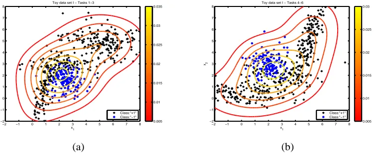
Figure 2: Toy data set I distribution; (a) scatter plot and density for the first cluster of tasks (1-3), (b) scatter plot and density for the second cluster of tasks (4-6).
4.1.1 TOYDATASETI
The first toy data set is comprised of six binary classification tasks. This toy problem was previously used in Liu et al. (2009) in the context of semi-supervised multi-task learning. Data for the first three tasks are generated from a mixture of two partially overlapping Gaussian distributions, and similarly for the remaining three tasks. Hence, the six tasks cluster in two groups; for each task 600 data points were generated, which were equally divided between the two classes. The scatter plots of the two clusters are shown in Figures 2.a and 2.b.
0 10 20 30 40 50 60 0.65
0.7 0.75 0.8 0.85 0.9 0.95 1
DPET
Average AP
Toy data set I
MTL BatchMCAppr P2PMCGat MAP Pool
1 2 3 4 5 6
1
2
3
4
5
6
Task
Task
Toy Data set I
(a) (b)
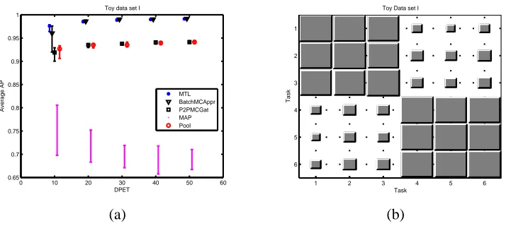
Figure 3: Toy data set I classification Results; (a) Average AP over the 6 tasks, (b) Hinton Diagram of the task covariance matrix of the CMTMC model computed by averaging over the 25 repetitions with 50 data points per task.
Classification results are presented in Figure 3.a; the Y axis is the AP, and the X axis is the number of data points from each task (DPET) used for training. The results show that, in this toy problem, the Batch mode performs similarly to the ideal MTL case, although it has a high variance for the case of 10 DPET. The P2PGat and Pooling method perform approximately 10% worse than the Batch, while the MAP estimate gives roughly 20% less than the Batch. Moreover, Figure 3.b
shown the Hinton diagram4 (Hinton, 1989) of the task covariance matrix of the CMTMC model
which accurately recovers the structure of the tasks.
4.1.2 TOYDATASETII
The second toy data set consists of four tasks which group into two clusters. The scatter plot as well as the density of the two clusters are shown in Figures 4.a and 4.b, for the first and second cluster respectively. The main feature of this data set, evident visually from Figure 4, is the similarity of the data generating distribution for the two tasks. While the densities are peaked in different locations, without class labels the tasks are almost identical, meaning that the multi-class classifier cannot learn to discriminate between the two tasks. As in the previous example, each task consisted of 600 data points equally divided between the two classes, and we used the ARD covariance function.
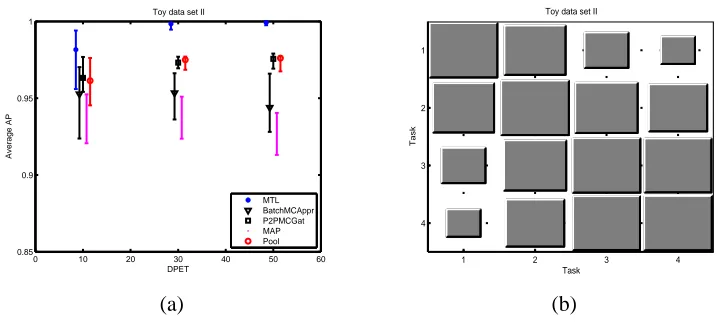
Figure 5.a shows the results the different methods produced. As expected, the Batch mode fails to correctly identify the task responsibilities; as a result, it gives a lower average AP than the MTL, a difference which does not decrease with the number of DPET, indicating statistical inconsistency. This is reinforced by the Hinton diagram of Kt in Figure 5.b, where it fails to identify the clusters of the tasks. Even though this difference is small it is significant for this easy problem, where the MTL algorithm performs close to 100%. Additionally, the P2PGat, the Pooling, and the MAP estimates perform better that the Batch, but they also fail to reach the performance of MTL.
−1 −0.8 −0.6 −0.4 −0.2 0 0.2 0.4 0.6 0.8 1 −1
−0.8 −0.6 −0.4 −0.2 0 0.2 0.4 0.6 0.8 1
x1
x2
Toy data set I − Tasks 1−2
Class:"+1" Class:"−1"
0.04 0.06 0.08 0.1 0.12 0.14 0.16 0.18 0.2 0.22 0.24
−1 −0.8 −0.6 −0.4 −0.2 0 0.2 0.4 0.6 0.8 1
−1 −0.8 −0.6 −0.4 −0.2 0 0.2 0.4 0.6 0.8 1
x1
x2
Toy data set II − Tasks 3−4
Class:"+1" Class:"−1"
0.04 0.06 0.08 0.1 0.12 0.14 0.16 0.18 0.2 0.22 0.24
(a) (b)
Figure 4: Toy data set II distribution;(a) scatter plot and density for the first cluster of tasks(1-2), (b) scatter plot and density for the second cluster of task(3-4).
4.1.3 CHARACTERCLASSIFICATION
In this data set the task is to learn to classify between commonly confused handwritten letters, which is included in the “Transfer learning Toolkit” of Berkeley University available at http://
multitask.cs.berkeley.edu/. This data set is comprised of eight binary classification tasks.
The characters that are used and the number of samples are given in Table 1. Each sample is a 16×8 image, which results into a binary 128 feature vector. The covariance function that is employed for this data set is the Radial Basis Function (RBF).
0 10 20 30 40 50 60
0.85 0.9 0.95 1
DPET
Average AP
Toy data set II
MTL BatchMCAppr P2PMCGat MAP Pool
1 2 3 4
1
2
3
4
Task
Task
Toy data set II
(a) (b)
Figure 5: Toy data set II classification Results; (a) Average AP over the 4 tasks, (b) Hinton Diagram of the task covariance matrix.
Task 1 2 3 4 5 6 7 8
Letter c g m a i a f h
Number of data 2017 2460 1596 4016 4895 4016 918 858
Letter e y n g j o t n
Number of data 4928 1218 5004 2460 188 3880 2131 5004
Table 1: Description of the Character data set; each column is a task showing the two letters as well as the corresponding number of examples per character.
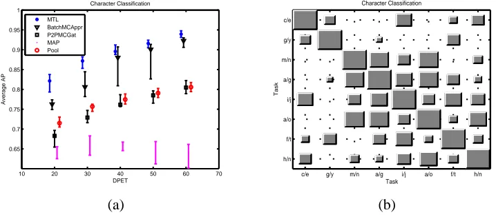
(although there is significant variability for small numbers of labeled data per task). Figure 6.b shows the Hinton diagram of the task covariance matrix, which indicates a more random structure between the tasks, but finds that some tasks are more correlated than others, for example ‘a/g’ with ‘a/o’, and ‘i/j’ with ‘f/t’. It should be noted though, that in this data set the “low-error joint prediction” assumption is partially violated since there is label disagreement between tasks ‘a/g’ and ‘g/y’, where the ‘g’ letter belongs to class “+1” in task ‘a/g’ and to “-1” in task ‘g/y’. This does not seem to have any adverse effect on the performance of the model, presumably as the difference between letters ‘a’ and ‘y’ is sufficient to unambiguously assign the target task to the correct source task.
10 20 30 40 50 60 70
0.65 0.7 0.75 0.8 0.85 0.9 0.95 1
DPET
Average AP
Character Classification MTL
BatchMCAppr P2PMCGat MAP Pool
c/e g/y m/n a/g i/j a/o f/t h/n
c/e
g/y
m/n
a/g
i/j
a/o
f/t
h/n
Task
Task
Character Classification
(a) (b)
Figure 6: Character Classification Results; (a) Average AP over the 8 tasks, (b) Hinton Diagram of the task covariance matrix.
4.1.4 ARRHYTHMIACLASSIFICATION
(2008) using single task GP classifiers. Each recording was sampled at 360Hz, and annotation pro-vided by the database was used to separate the beats before any preprocessing. Each beat segment, consisting of 360 data points (one minute), was transformed into the frequency domain using a Fast Fourier Transform with a Hanning window. Only the first ten harmonics are used as features for classifying heart beats, as most of the information of the signal is contained in these harmonics.
Recording ID 106 200 203 217 221 223 233
Total number of data 2021 2567 2970 406 2349 2417 3053
Number of Normal heart beats 1503 1740 2526 244 1954 1955 2224
Number of PVC heart beats 518 827 444 162 395 462 829
Table 2: Description of the Arrhythmia data set.
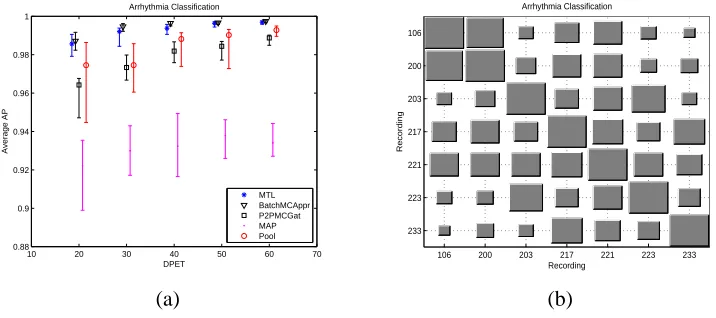
Figure 7.a shows the average AP over the seven tasks. On average, the Batch method performs better than the P2PMCGat, the MAP, and the Pool, while it presents a small advantage compared to MTL. Interestingly, the MAP approach is consistently worse than other methods, a situation that will be reversed in the partially observed tasks scenario. As in the character classification problem the task covariance matrix Kt, shown in Figure 7.b, demonstrates that there are correlations between the tasks but in more random way.
10 20 30 40 50 60 70
0.88 0.9 0.92 0.94 0.96 0.98 1
DPET
Average AP
Arrhythmia Classification
MTL BatchMCAppr P2PMCGat MAP Pool
106 200 203 217 221 223 233
106
200
203
217
221
223
233
Recording
Recording
Arrhythmia Classification
(a) (b)
Figure 7: Arrhythmia Classification Results; (a) Average AP over the 7 tasks, (b) Hinton Diagram of the task covariance matrix.
4.1.5 OBSERVATIONS
This set of experiments has demonstrated the effectiveness of the CMTMC model in situations where the data distribution of the target task comes from one of the source tasks. Several observa-tions are made:
points are needed to produce an accurate estimate of the density of the target task. This is empirically confirmed in our investigation, as Batch closely approaches the MTL results in all cases.
2. If the “low-error joint prediction” assumption is violated, then meta-generalising becomes a very hard problem, possible unsolvable. The performance on the second toy example was not particularly bad, since all methods achieved higher that 90% in terms of AP, but none of methods reached the performance of the MTL algorithm, and the performance did not appre-ciably improve when more training data were provided, indicating statistical inconsistency. This effect could be dramatically increased if for example the classes between the clusters were anti-correlated, so that similar data generating distributions could be potentially associ-ated with opposite predictions. Note though that if discriminative task descriptor features are available then this problem can be overcome, because augmenting the feature space would result in a different mapping of the latent function f .
3. If the model assumptions are met, the correlation structure of the tasks does not have a strong influence on the predictions, since the Batch mode outperformed the P2PGat gating and MAP estimate in all experiments. As we will see, this will be a crucial difference between the fully and partially observed tasks scenario.
4.2 Partially Observed Tasks
We now consider the harder problem of making predictions on completely unseen tasks. In this case, a priori we have no guarantee that any of the underlying modelling assumptions (similarity of distribution and low-error joint prediction) may hold. However, in some situations it is not unrealistic to assume that inter-task correlations will be structured, for example by the presence of
clusters of similar tasks. These clusters may be evident from the experimental design of the problem
(as in the case of the landmine data set discussed below), or may become evident from the training phase on the source tasks, if the learned task covariance matrix exhibits a strong block structure.
We are not aware of other methods that has a distribution matching mechanism to perform predictions on totally unseen tasks. Therefore, in this section we will only compare the different inference mechanisms of the CMTMC model (Batch and P2PGat) with a GP model trained by pooling all data together and with the MAP combination of classifiers.
4.2.1 TOYDATASETI
100 150 200 0.65
0.7 0.75 0.8 0.85 0.9 0.95 1
DPET
Average AP
Training on "2" tasks, generalizing on "4"
BatchMCAppr P2PMCGat MAP Pool
100 150 200
0.65 0.7 0.75 0.8 0.85 0.9 0.95 1
DPET
Average AP
Training on "4" tasks, generalizing on "2"
BatchMCAppr P2PMCGat MAP Pool
(a) (b)
Figure 8: Average AP on the unseen tasks of Toy data set I; (a) training on 2 tasks generalising on 4, (b) training on 4 tasks generalising on 2.
sizes. Comparing the performance of the Toy data set I in the fully and partially observed cases, in Figures 3 and 8 respectively, reveals that the same levels of AUC are achieved in both experimental setups, indicating that the task classification GP is highly confident of the correct result.
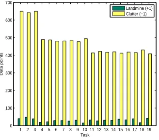
4.2.2 LANDMINEDETECTION
The landmine detection data set consists of images measured with airborne radar systems, and the goal is to predict landmines or clutter (Xue et al., 2007). Data are collected from 19 landmine fields, which are considered as subtasks, and each point is represented by a nine-dimensional feature vector. Tasks 1-10 correspond to regions that are relatively highly foliated while tasks 11-19 correspond to regions that are bare earth or desert. Figure 9 shows the number of data points from each task and each class, which indicates that this data set is highly imbalanced in favor of the Clutter (‘-1’) class. The experimental setup suggests the presence of two clusters of tasks corresponding to the
1 2 3 4 5 6 7 8 9 10 11 12 13 14 15 16 17 18 19 0
100 200 300 400 500 600 700
Task
Data points
Landmine (+1) Clutter (−1)
geomorphology of the region the observations come from; this is confirmed by our preliminary investigation (not shown), as well as from previously published results on this data set by Xue et al. (2007) and Liu et al. (2009). Thus, in this data set training tasks are set by randomly selecting equal number of tasks from the first cluster, tasks 1-10, and from the second cluster, tasks 11-19. Experiments are presented for two, four, and eight training tasks. The data covariance function that is used for this data set is the ARD.
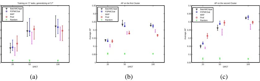
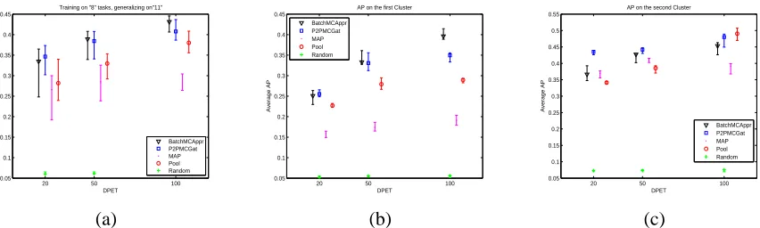
Figures 10.a, 11.a, and 12.a shows the mean AP on the 17, 15, and 11 unseen target tasks for each partition respectively. Due to the high imbalance between the classes (Landmine-Clutter) the achieved AP of all methods is very low. Therefore, in this data set we also present the AP of a random predictor which clearly shows the improvement of each method considered. Note that in terms of AUC the results obtained in this work are consistent with previous studies in this data set (Xue et al., 2007; Liu et al., 2009), which are presented in Appendix C Figure 14 for completeness. Moreover, it is noticed that there are large overlapping error bars between all methods. Large error bars give evidence that there might be two levels of performance. Therefore, for each partition we provide the average AP for each cluster separately; subfigures (b) from Figures 10, 11, and 12 show the average AP for the first cluster, and subfigures (c) for the second cluster. Measuring the AP in each cluster separately gives significantly smaller error bars, and reveals interesting structures in the problem. Specifically, the performance on the second cluster is always better than on the first cluster by a considerable margin. Moreover, comparing the methods on each cluster separately we see that the Batch method outperformed the pooling and the P2PGat in most of the cases, particularly in the first cluster where the advantages become very significant as we increase the number of tasks/ DPETs. The correlation structure within the second cluster is looser, immplying a weaker applica-bility of our modelling assumptions. However it should be pointed out that this is a substantially harder pattern recognition task compared to the toy data set considered above. For example, Liu et al. (2009) that investigated the application of semi-supervised MTL on this data set achieved a best performance of 78% AUC; the CMTMC (which relies on the more flexible GP framework for MTL) achieves an average AUC above 76% on totally unseen tasks having trained on only 8 source tasks with 100 DPET (see Figure 14).
20 50 100
0.05 0.1 0.15 0.2 0.25 0.3 0.35 0.4
DPET
Average AP
Training on "2" tasks, generalizing on"17"
BatchMCAppr P2PMCGat MAP Pool Random
20 50 100
0 0.05 0.1 0.15 0.2 0.25 0.3 0.35
DPET
Average AP
AP on the first Cluster
BatchMCAppr P2PMCGat MAP Pool Random
20 50 100
0.05 0.1 0.15 0.2 0.25 0.3 0.35 0.4
DPET
Average AP
AP on the second Cluster
BatchMCAppr P2PMCGat MAP Pool Random
(a) (b) (c)
20 50 100 0.05 0.1 0.15 0.2 0.25 0.3 0.35 0.4 0.45 DPET Average AP
Training on "4" tasks, generalizing on"15"
BatchMCAppr P2PMCGat MAP Pool Random
20 50 100
0.05 0.1 0.15 0.2 0.25 0.3 0.35 0.4 DPET Average AP
AP on the first Cluster
BatchMCAppr P2PMCGat MAP Pool Random
20 50 100
0.05 0.1 0.15 0.2 0.25 0.3 0.35 0.4 0.45 DPET Average AP
AP on the second Cluster
BatchMCAppr P2PMCGat MAP Pool Random
(a) (b) (c)
Figure 11: Average AP on the 15 unseen tasks of Landmine data set; training on 4 tasks, generalis-ing on 15; (a) Overall AP over 15 tasks, (b) Average AP over 8 tasks of the first cluster, (c) Average AP over 7 tasks of the second cluster.
20 50 100
0.05 0.1 0.15 0.2 0.25 0.3 0.35 0.4 0.45 DPET Average AP
Training on "8" tasks, generalizing on"11"
BatchMCAppr P2PMCGat MAP Pool Random
20 50 100
0.05 0.1 0.15 0.2 0.25 0.3 0.35 0.4 0.45 DPET Average AP
AP on the first Cluster
BatchMCAppr P2PMCGat MAP Pool Random
20 50 100
0.05 0.1 0.15 0.2 0.25 0.3 0.35 0.4 0.45 0.5 0.55 DPET Average AP
AP on the second Cluster
BatchMCAppr P2PMCGat MAP Pool Random
(a) (b) (c)
Figure 12: Average AP on the 11 unseen tasks of Landmine data set; training on 8 tasks, generalis-ing on 11; (a) Overall AP over 11 tasks, (b) Average AP over 6 tasks of the first cluster, (c) Average AP over 5 tasks of the second cluster.
4.2.3 ARRHYTHMIACLASSIFICATION
As a second real data set, we return to the arrhythmia classification problem introduced in Section 4.1.4. The results from the fully observed tasks scenario indicate an unclear pattern of correlations between the tasks, as summarised in the task covariance matrix Figure 7.b, which calls into question the validity of the similarity of distribution assumption. Fortunately, in this application the classes have a physical interpretation. For example normal heart beats between different patients, although not exactly the same, can be expected to be similar, and a PVC arrhythmic heart beat of one patient can not have the wave form of a normal heart beat from another patient. This allows us to assume that the classes between the tasks will not be anti-correlated, so that at least the low-error joint prediction assumption should approximately hold.
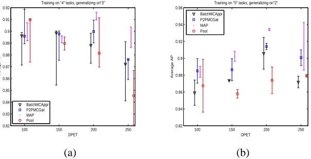
lot lower than in the fully observed case, something perhaps to be expected since, contrary to the previous two examples, the model assumptions are not fully met in this data set. Surprisingly, the method that achieved the best performance was the MAP, and no principled justification can be given for that. Secondly, we observe that the performance in this set of experiments exhibits some interesting patterns as the number of training tasks increases. Specifically, for four training tasks the performance of all methods does not significantly improve as we increase the number of data points per task, and in some cases it even deteriorates, a phenomenon that was also observed for 2 and 3 training tasks but results are omitted for brevity. This indicates that if the space of tasks has not been sampled sufficiently, the model can not yield good generalisation performance to new tasks, even if the number of training data increases. In contrast, for five training tasks the MAP and P2PGat methods yield a significant improvement of performance as the number of data points increases (levelling off after 200 DPETs).
100 150 200 250
0.82 0.83 0.84 0.85 0.86 0.87 0.88 0.89 0.9 0.91 0.92
DPET
Average AP
Training on "4" tasks, generalizing on"3"
BatchMCAppr P2PMCGat MAP Pool
100 150 200 250
0.82 0.84 0.86 0.88 0.9 0.92 0.94 0.96
DPET
Average AP
Training on "5" tasks, generalizing on"2" BatchMCAppr
P2PMCGat MAP Pool
(a) (b)
Figure 13: Average AP on the unseen tasks of Arrhythmia data set on different number of training tasks; (a) training on 4 tasks, generalising on 3, (b) training on 5 tasks, generalising on 2.
Empirically, it would appear that the P2PGat method is preferable to the Batch method when the model assumptions are violated. Intuitively, one could argue that the Batch method is less flexible, as the relative contribution of the different single-class predictors is fixed across all points in the target task. Therefore, if the model assumptions are violated, leading to an incorrect task labelling, the propagated error could have a worse effect in Batch than in P2PGat. This is partly confirmed by the analysis of Toy data set II in Section 4.1.2, where the model assumptions were violated and P2PGat gave significantly higher AP than the Batch method.
4.2.4 CHARACTERCLASSIFICATION
for task ‘a/g’, and to the positive class for task ‘g/y’. Therefore, the character classification problem is ill-suited for this type of experiments. This is borne out by experimental evidence: simulation results with 4, 5, and 6 training tasks, which are omitted for brevity, indicated that increasing the number of tasks and the number of training points per task does not improve the performance in any of the methods. Specifically, the results obtained were close to that of a random predictor indicating statistical inconsistency of the model assumptions with the data.
4.2.5 OBSERVATIONS
Meta-generalising in a partially observed tasks scenario is an extremely hard problem; neverthe-less, we believe there are some interesting points that can be made from the previous experimental analysis. Below we summarise the most important observations for this scenario.
1. In situations where there are clusters of tasks, even though the model hasn’t seen all tasks, the Batch method can still make accurate predictions that reaches the performance of the fully observed tasks case. Pragmatically, one could consider whether the training phase of the model has revealed clusters of tasks when deciding which prediction method to apply.
2. In multi-task problems where the correlations between the tasks are less pronounced, but where the low-error joint prediction is satisfied and where a sufficient number of training tasks is available, the method that is most appropriate is the P2PGat, since it provides a more flexible task assignment mechanism than the Batch mode. The validity of the low-error joint prediction assumption can sometimes be assessed from the nature of the problem (as in the arrhythmia case).
3. Sufficient exploration of the task space is essential for the success of the method. While we have not tested our model for very large numbers of training tasks, the results suggest that often a significant improvement in performance can be achieved when the number of training tasks crosses a critical number, indicating a sufficient coverage of the task space. This phenomenon was observed in the Arrhythmia classification problem for 2 and 3 training tasks where the performance of the models remained the same as the number of training samples per task increased. In essence more training data lead to stronger biases for meta-generalisation in target tasks that are not correlated with any of the training tasks.
4. In most cases, when the assumptions of the model are only approximately met and when the exploration of the task space is insufficient, the generalisation performance on totally unseen tasks is still modest, and it may be that other approaches based on mixtures of GP experts (Tresp, 2000) achieve similar results. An extensive comparison with these approaches would be interesting, but outside the scope of the present work.
5. Conclusions