Value Regularization and Fenchel Duality

Value Regularization and Fenchel Duality

Ryan M. Rifkin [email protected]

Honda Research Institute USA, Inc. One Cambridge Center, Suite 401 Cambridge, MA 02142, USA

Ross A. Lippert [email protected]

Department of Mathematics

Massachusetts Institute of Technology 77 Massachusetts Avenue

Cambridge, MA 02139-4307, USA

Editor: Peter Bartlett

Abstract

Regularization is an approach to function learning that balances fit and smoothness. In practice, we search for a function f with a finite representation f =∑iciφi(·). In most treatments, the ci are the primary objects of study. We consider value regularization, constructing optimization prob-lems in which the predicted values at the training points are the primary variables, and therefore the central objects of study. Although this is a simple change, it has profound consequences. From convex conjugacy and the theory of Fenchel duality, we derive separate optimality conditions for the regularization and loss portions of the learning problem; this technique yields clean and short derivations of standard algorithms. This framework is ideally suited to studying many other phe-nomena at the intersection of learning theory and optimization. We obtain a value-based variant of the representer theorem, which underscores the transductive nature of regularization in repro-ducing kernel Hilbert spaces. We unify and extend previous results on learning kernel functions, with very simple proofs. We analyze the use of unregularized bias terms in optimization problems, and low-rank approximations to kernel matrices, obtaining new results in these areas. In summary, the combination of value regularization and Fenchel duality are valuable tools for studying the optimization problems in machine learning.

Keywords: kernel machines, duality, optimization, convex analysis, kernel learning

1. Introduction

Given a set of training data_{(X1,Y1), . . . ,(Xn,Yn)}, the inductive supervised learning task is to learn

a function f that, given a new X value, will predict the associated Y value. A common framework for solving this problem is Tikhonov regularization (Tikhonov and Arsenin, 1977):

inf

f_∈F

(

n

∑

i=1

v(f(Xi),Yi) +

λ 2Ω(f)

)

. (1)

In this general form,

F

is the loss, indicating the penalty we pay when we see Xi, predict f(Xi), and the true value is Yi. For

a large class of functions

F

that penalizes elements of f that are too “complex”. The regularization parameter,λ, controls the tradeoff between finding a function of low complexity and fitting the training data.

A large amount of work (Wahba, 1990; Evgeniou et al., 2000) takes

F

H

inf

f∈H (

n

∑

i=1

v(f(Xi),Yi) +

λ 2||f||

2

k

)

, (2)

indicating that the regularization term is now the squared norm of the function in the RKHS. Many common algorithms, including support vector machines for classification (Cortes and Vapnik, 1995) and regression (Vapnik, 1998), regularized least squares (Wahba, 1990; Poggio and Girosi, 1990; Rifkin, 2002), and kernel logistic regression (Jaakkola and Haussler, 1999) are instances of Tikhonov regularization: different loss functions yield different algorithms.1

A consequence of the so-called representer theorem (Wahba, 1990; Sch ¨olkopf et al., 2001), is that the minimizer of (2) will have the form

f(x) =

n

∑

i=1

cik(x,Xi). (3)

In other words, in an RKHS, a function f which minimizes (2) is a sum of kernel functions k(_·,Xi)

over the data points. We solve a Tikhonov regularization (or, equivalently, train a predictor) by finding the coefficients ci. Assuming that the loss function is convex, the minimization of (2) (or

(1)) is tractable.

Defining K as the n_×n kernel matrix with Ki j =k(Xi,Xj), the regularization penalty ||f||2_k

becomes ctKc, the output at training point i is given by f(Xi) =∑nj=1cjk(Xi,Xj) = (Kc)i, and we

can rewrite (2) as

inf

c_∈Rn

(

n

∑

i=1

v((Kc)i,Yi) +

λ 2c

t_Kc

)

. (4)

Regularizing in an RKHS is special in that it has a representer theorem: the optimal solution in an infinite-dimensional space of functions is found by solving a finite dimensional minimization problem. Although most other function space regularizers do not have similar properties, we may consider other regularizers as modifications of (4): replacing ctKc with ctc, we obtain ridge re-gression (Tikhonov and Arsenin, 1977), and replacing it with∑n_i=1|ci|, we obtain L1-regularization

(Zhu et al., 2003). In such cases, we are assuming that we are looking for a function of the form (3) a priori. There is nothing wrong with this, but it should not be confused with the case of RKHS regularization, where (3) arises naturally from a search for an optimizing function.

In general, an equation like (4) is used as the starting point for thinking algorithmically about finding c. For example, in a standard development of support vector machines (Cristianini and Shaw-Taylor, 2000; Rifkin, 2002), one starts with (4) instantiated with the SVM hinge loss v(f(Xi),Yi) = (1−yif(Xi))+, introducing slack variablesξi=v(f(Xi),Yi)and constraints to handle

the non-differentiability of the hinge loss at 0 as well as an unregularized bias term b, yielding a quadratic program:2

min

c∈Rn_,ξ∈Rn_,b∈R

1

n∑ n

i=1ξi+λcTKc

subject to : Yi ∑nj=1cjk(Xi,Xj) +b

≥1₋ξi i=1, . . . ,n

ξi≥0 i=1, . . . ,n.

This program is called the primal problem. In order to expose sparsity in the solution, the La-grangian dual is taken, yielding the dual problem:

max

α∈Rn ∑ n

i=1αi−₍₂1_λ)2αtdiag(Y)Kdiag(Y)α

subject to : ∑n_i=1Yiαi=0

0_≤αi≤1_n i=1, . . . ,n.

It is then observed that the dual problem is easier to solve (because of its simpler constraint struc-ture), and that solutions to the primal can be easily obtained from solutions to the dual.

We propose to take a different approach to Tikhonov regularization, that we believe to be more fundamental. The approach rests on two ideas.

First, we consider the predicted values yi≡ f(Xi) = (Kc)ito be the central objects of study, and

write our optimization problems in terms of y. In the case of RKHS regularization with a positive-definite kernel, the matrix K is typically non-singular (Micchelli, 1986), 3 and we rewrite (4) as a value regularization:

inf

y_∈Rn

(

λ 2y

t_K−1_y+

∑

i=1 v(yi,Yi)

)

.

Although this is a simple transformation, the consequences are far-reaching. Looking at the rewrit-ten problem, we notice that the kernel matrix K appears only in the regularization—it does not appear in the loss term. This is intuitive, as the loss function (of course) cares only about the predicted outputs, not what combination of kernel coefficients generated those predicted outputs. Additionally, we see that the loss function decomposes into n separate single-point loss functions. In contrast, if the ciare the primary variables, the loss at each data point is a function of the entire c

vector.

The benefits of value regularization are greatly amplified by the second central idea of this work: instead of Lagrangian duality, we use Fenchel duality (Borwein and Lewis, 2000), a form of duality that is well-matched to the problems of learning theory. Although we discuss Fenchel duality in greater detail below, we present a brief overview here. Consider an optimization problem of the form:

inf

y∈Rn{f(y) +g(y)}. (5)

2. Traditional derivations parametrize the loss function instead of the regularization, with a constant C= 1

2λ, but that is

a minor point.

Fenchel duality defines a so-called Fenchel dual:

sup

z∈Rn{−

f∗(z)₋g∗(₋z)_}, (6)

where f∗,g∗are Fenchel-Legendre conjugates (definition 4) computed via auxiliary (and by design, simpler) optimization problems on f and g separately. Convexity of f and g (and some topological qualifications) ensure that the optimal objective values of (5) and (6) are equivalent, and that any optimal y and z satisfy:

f(y)₋ytz+f∗(z) = 0

g(y) +ytz+g∗(₋z) = 0.

Fenchel duality encompasses other notions of duality such as Lagrangian duality and seems to be a natural concept to apply to regularization problems where f and g each arise from different considerations—for supervised learning problems, one will come from regularization and the other from empirical loss.

Elaborating on this idea, Fenchel duality gives us a separation of concerns which is not present in the Lagrangian approach. The point of formulating an optimization problem such as a quadratic program is ultimately to derive optimality conditions and algorithms for finding optimal solutions. For convex optimization problems, all local optima are globally optimal, and we can formulate a complete set of optimality conditions which the primal and dual solutions will simultaneously satisfy. These are generally known as the Karush-Kuhn-Tucker (KKT) conditions (Bazaraa et al., 1993).4 Fenchel duality makes it clear that the two functions f and g, or, in our case, the loss term and the regularization, contribute individual local optimality conditions, and the total optimality conditions for the overall problem are simply the union of the individual optimality conditions. Put differently, using Fenchel duality, we can derive a table for nr regularizations and nl losses,

and immediately combine these to derive optimality conditions for nrnl learning problems. This

idea is obscured by the Lagrangian duality approach to deriving optimality conditions for learning problems. As an example, for the common case of the RKHS regularizer 1₂ytK−1y, we will find that the primal-dual relationship is given by y=λ−1_{Kz. This condition is independent of the loss—it} shows up simultaneously in SVM, regularized least squares, and logistic regression.

Value regularization and Fenchel duality reinforce each other’s strengths. Because the kernel affects only the regularization term and not the loss term, applying Fenchel duality to value regular-ization yields extremely clean formulations. The major contribution of this paper is the combination of value regularization and Fenchel duality in a framework that yields new insights into many of the optimization problems that arise in learning theory.

We present, in Section 3, a primer on convex analysis and Fenchel duality, with emphasis on the key ideas that are needed for learning theory. We believe that this section provides a sufficiently self-contained summary of convex analysis to allow a machine learning researcher to apply our framework to new problems.

In Section 4, we specialize the convex analysis results to Tikhonov value regularizations con-sisting of the sum of a regularization and a loss term. Section 5 specializes the result further to the RKHS case and obtains very simple derivations of well-known kernel machines.

Section 6 is concerned with value regularization in the context of L1 regularization, a regular-ization with the explicit goal of obtaining sparsity in the finite representation. In Section 6.1, we

briefly discuss 1-norm support vector machines, and emphasize a key distinction between RKHS and other regularizations: in RKHS regularization, the ci, which are the expansion coefficients in

the finite representation of the learned function, and the zi, which are the dual variables associated

with the yi in the value regularization problem, are identifiable (z=λ−1c). This is a consequence

of the RKHS regularization, and does not hold for more general regularizations. In Section 6.2, we present a simpler derivation of the relationship between support vector regression and sparse ap-proximation, first discovered in Girosi (1998); essentially, the problems are duals, with the width of theε-tube in the support vector regression problem becoming the sparsity regularizer in the sparse approximation problem.

In Section 7, we develop a new view of the representer theorem, in the context of value regular-ization. The common wisdom about the representer theorem is that it guarantees that the solution to an optimization problem in an (infinite-dimensional) function space has a finite representation as an expansion of kernel functions around the training points. While this is certainly true, we gain additional insights by considering an augmented problem in which the test points also appear in the regularization, but not in the loss. In the augmented optimization problem the predicted out-puts at the training points do not change, and the expansion coefficients at the test points vanish—a representer theorem. This underscores the fact that for supervised learning in an RKHS, induction and transduction are identical. In the context of transductive or semi-supervised algorithms, the picture is more complex. There have been several recent articles that turn transductive algorithms into semi-supervised algorithms via an appeal to the representer theorem. While this is formally valid, the resulting transductive algorithm is not equivalent to the semi-supervised algorithm, and the transductive algorithm is perhaps the more “natural” choice. Section 7.1 is devoted to a discus-sion of this topic.

Recently, there has been interest in “learning the kernel”. In Section 8, we may view this as a value regularization where the kernel matrix itself is an auxiliary parameter to be optimized. The value-based formulation is ideal here, because the kernel appears only in the regularization term and not in the loss term. We first derive a general result that gives optimality conditions for a general convex penalty F(K) on the kernel matrix. Work to date has considered only the case where F is 0 for some set of semi-definite matrices, and infinite otherwise. Lanckriet et al. (2004) considers a case where the kernel function is a linear combination of a finite set of kernels; we will see that a minor modification to their formulation yields a representer theorem and an agreement of inductive and transductive algorithms. Argyriou et al. (2005) work with a convex set generated by an infinite, continuously parametrized set of kernel functions. We give proofs of their main results which are shorter and simpler, and also more general, allowing arbitrary convex loss functions (Argyriou et al. (2005) requires differentiability).

In Section 9, we show how infimal convolutions, a form of optimization relaxation (see Section 3.4) are useful in learning theory. We first explore the idea of “biased” regularizations, the best-known example being the unregularized bias term b in the standard formulation of support vector machines. We show that unregularized bias terms arise from infimal convolutions and that the optimality conditions implied by bias terms are independent of both the particular loss function and the particular regularization. For example, including an unregularized constant term b in any Tikhonov optimization problem yields a constraint on the dual variables ∑zi=0; this constraint

arbitrary convex set. In Section 9.2, we see that the computation of leave-one-out values can also be viewed as a biased regularization via infimal convolution.

In Section 10, we explore low rank kernel matrix approximations such as the Nystr ¨om ap-proximation, which consists of picking a partition N_∪M of the data, and approximating K with

˜ K=

KNN KNM

KMN KNMKMM−1KMN

. In Willams and Seeger (2000), the authors suggest using ˜K in place

of K. Several authors (Rifkin, 2002; Rasmusen and Williams, 2006) have found empirically that this works poorly, but that a closely related approach (the subset of regressors method) of constraining ci to be zero for points not in the subset M works quite well. These two approaches are extremely

closely related mathematically. With value regularization and Fenchel duality, we explore in detail the relation between these methods. The subset of regressors method is, in some sense, the “natu-ral” algorithm arising from the low-rank matrix approximation, while the Nystr ¨om method makes an unwarranted identification of the dual variables, z, and the coefficients of expansion in the finite representation, c.

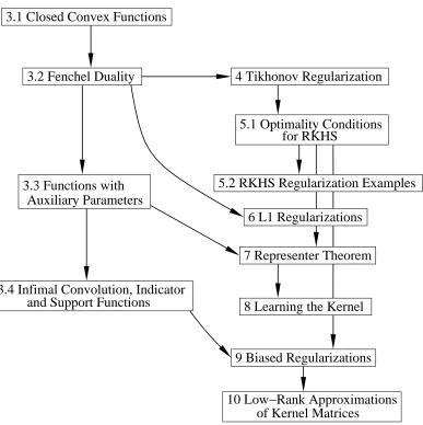
The framework presented here requires a moderate mathematical investment by the reader. For this reason, we have organized the paper so that the material on convex analysis (Section 3) can be digested in several chunks and give a roadmap (Figure 1) to illustrate which sections are accessible using only a subset of Section 3. Additionally, in Section 3.5, we provide a cheat sheet of key ideas from convex analysis, stated without their full qualifying conditions. Alternatively, readers may use the roadmap to skip unnecessary review.

Fenchel duality will find many uses in machine learning theory. Very recently (while the present paper was under review), Dud´ık and Schapire (2006) used Fenchel duality to explore maximum entropy distribution estimation under constraints, and Altun and Smola (2006) explored relations between divergence minimization and statistical inference. In summary, Fenchel duality is a pow-erful way to look at the regularization problems that arise in learning theory. While it requires some mathematical sophistication, the resulting formulations are elegant and yield new insights. We hope that many people will find this approach useful.

2. Notation

A training set is a set of labelled points_{(X1,Y1), . . . ,(Xn,Yn)}. We will sometimes use N to refer

to the set_{x1, . . . ,xn}, and we may have an additional set of (unlabelled) points of size m called M

(e.g., N=_{X1, . . . ,Xn}and M={Xn+1, . . . ,Xn+m}).

Throughout this paper, Yi (capitalized) refers to given labels for training points. yiare variables

that we optimize over. In general, we can imagine that we are learning a function f , and yi= f(Xi),

but we generally think of optimizing the yidirectly rather than using f as an intermediary.

Beginning in Section 3, we will frequently take Fenchel-Legendre conjugates and use z to denote variables conjugate to y (i.e., we are using z to refer to “dual variables”). We will also sometimes obtain functions of the form f(x) =∑icik(Xi,x) and exclusively use ci to refer to the expansion

coefficients in the finite representation of f .

We define ei to be the n-vector whose ith entry is 1 and whose other entries are zero: the ith

basis vector in the standard basis forRn_{(n will always be clear from context). We define 1}

nto be a

vector of length n whose entries are all 1.

We use H to refer to affine (or hyperplane) functions, Hv,c(y) =vty−c. For any symmetric

and Support Functions

for RKHS

5.1 Optimality Conditions

of Kernel Matrices

10 Low−Rank Approximations

3.2 Fenchel Duality

9 Biased Regularizations

6 L1 Regularizations

8 Learning the Kernel

7 Representer Theorem

5.2 RKHS Regularization Examples

4 Tikhonov Regularization

3.1 Closed Convex Functions

Auxiliary Parameters

3.3 Functions with

3.4 Infimal Convolution, Indicator

Figure 1: A roadmap of this paper. The sections on convex analysis are in the left-hand column, while the “applications” are in the right-hand column.

If S,S0_⊂Rnand A_∈Rm×n, then S+S0=_{y+y0: y_∈S,y0_∈S0_}, S₋S0=_{y₋y0: y_∈S,y0_∈S0_}, SS0=_{yy0 : y_∈S,y0_∈S0_}, and AS=_{Ay : y_∈S_}. In particular, ARn is the column space of A. We denote the topological interior of S_⊂Rn by int(S). A cone is a set S with the property that

R≥0S⊂S.

We writeBp⊂RnwhereBp={y∈Rn:||y||p≤1}where|| · ||pis the p-norm. We write A†for

the pseudoinverse of a matrix A.

3. Convex Analysis

Rockafellar and Wets (2004), although in some cases we have substituted less general versions of the results that are sufficient for our purposes, and in some cases we have elaborated (with proofs) ideas that are introduced as exercises in these books.

3.1 Closed Convex Functions

Definition 1 Given a function f :Rn→[₋∞,∞], the epigraph of f , epi f , is defined by epi f =_{(y,e): e_≥ f(y)_{} ⊂}Rn×R.

We say f is closed or convex if epi f is closed, or convex. We define dom f =_{y_∈Rn: f(y)<∞_}.

We say f is proper when dom f ₆=/0and f>₋∞(i.e.,_∀y,f(y)>₋∞). (Some texts consider f :Rn→(₋∞,∞], whereupon f >₋∞is automatic.)

We will mostly be considering f which do not take the value₋∞(such functions are somewhat pathological), in which case f being proper is equivalent to dom f ₆= /0. Allowing f to take the value of ∞ merely allows some portions of epi f to have no projection onto Rn (dom f is that projection). One way of viewing constrained minimization problems is as unconstrained problems with an objective function that can take the value∞. Indicator functions (introduced in Section 3.4) are a device for this purpose. We will not do arithmetic involving∞except where the result is unambiguous (e.g.,∞+1=∞).

The functions of primary interest to us are closed, convex, proper functions. We will call such a function a ccp function.

Definition 2 Given f :Rn→(₋∞,∞], we define the set argmin_y∈Rn f(y)as follows,

argmin

y∈Rn

f(y) =







Rn infy∈Rn f(y) =∞

{y : f(y) = f0} infy∈Rn f(y) = f₀∈R

/0 infy∈Rn f(y) =−∞

with symmetrical definitions for argmax when needed.

If f is proper, then the first case cannot occur. The occurrence of the middle case (given f proper) is equivalent to f being bounded from below. However, even in the second case, argmin_y f(y)may still be empty.

The notion of a supporting hyperplane gives us a non-smooth generalization of the gradient, called a subgradient.

Definition 3 (subgradients and subdifferentials) If f :Rn_→(−∞_,∞_{]is convex and y∈dom f ,}

thenφ_∈Rnis a subgradient of f at y if it satisfiesφtz_≤ f(y+z)₋f(y)for all z_∈Rn.

The set of all such φis the subdifferential and denoted ∂f(y). By convention, ∂f(y) = /0 if y_∈/dom f .

f

(

y

₀

)

y

₀

−

f

∗

(

z

)

H

_z,

_f

₍

_z

₎

(

y

) =

zy

−

f

∗

(

z

)

(

y

₀

,

f

(

y

₀

))

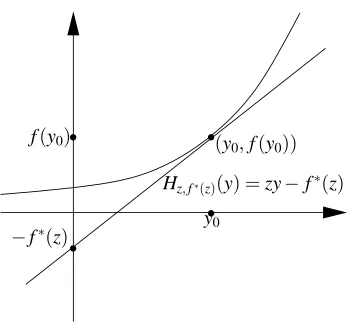
Figure 2: A graphical illustration of the Fenchel-Legendre conjugate.

3.2 Fenchel Duality

Central to Fenchel duality is the Fenchel-Legendre conjugate,

Definition 4 (Fenchel-Legendre conjugate) Given a function f : Rn → [₋∞,∞], the Fenchel-Legendre conjugate is

f∗(z) =sup

y {

ytz₋f(y)_}. (7)

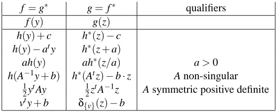
Table 1 lists a few general, easily derived conjugation identities.

For a convex function f of one variable, one can get a sense of what the conjugate and subgra-dient look like by examining a graph of f(y). For a given y, one finds a point(y0,f(y0))(on the boundary of epi f ) such that epi f is supported at y0by a line of the form Hz,c(y) =zy−c (i.e., z is

f=g∗ g=f∗ qualifiers f(y) g(z)

h(y) +c h∗(z)₋c h(y)₋aty h∗(z+a)

ah(y) ah∗(z/a) a>0 h(A−1y+b) h∗(Atz)₋b_·z A non-singular

1 2ytAy

1

2ztA−1z A symmetric positive definite vty+b δ_{v}(z)−b

Table 1: Some conjugates and properties of conjugation.

More generally, we can work in terms of affine functions and epigraphs. Equation 7 is equivalent to

epi f∗= \

y∈dom f

epi H_y,f(y).

Being an arbitrary intersection of closed and convex sets, epi f∗is closed and convex. Thus, f∗is closed and convex even if f is neither. Additionally, for z_∈dom f∗, by (7), we have Hz,f∗_(z)(y) =

zty₋f∗(z)_≤ f(y)for all y, and hence,

epi f _⊂ \

z∈dom f∗

epi Hz,f∗_(z),

holding with equality when f is closed and convex (Theorem 4.2.1 of Borwein and Lewis, 2000).

Theorem 5 (biconjugation) f :Rn→(₋∞,∞]is closed and convex iff f∗∗= f . In particular, conjugation is a bijection between ccp functions.

The supremum in (7) is attained if and only if Hz,f∗_(z)(y) = f(y)for some y. Thus, z∈∂f(y)is

equivalent to f(y) =yt_z−f∗_{(z)(Theorem 3.3.4 of Borwein and Lewis, 2000).}

Theorem 6 (Fenchel-Young) Let f :Rn→(₋∞,∞]be convex._∀y,z_∈Rn, f(y) +f∗(z)_≥ytz

with equality holding iff z_∈∂f(y).

Combining the previous results, if f is closed and convex then z_∈∂f(y)_⇔ y_∈∂f∗(z), and if z_∈int(dom f∗)the supremum in (7) is attained.

Fenchel duality can be motivated from Theorem 6 by considering two functions simultaneously. Given convex f,g :Rn→(₋∞,∞]

f(y) +f∗(z)₋ytz _≥ 0 (8)

g(y) +g∗(₋z)₋yt(₋z) _≥ 0. (9)

Summing the above inequalities and minimizing,

f(y) +g(y) + f∗(z) +g∗(₋z) _≥ 0 (10) inf

y {f(y) +g(y)}+infz {f

If ∃y,z∈Rn such that (10) is an equality, then clearly (11) holds with equality as well and the individual infima are attained. Moreover, (8) and (9) become equalities and thus z_∈∂f(y) and −z_∈∂g(y) (and y_∈∂f∗(z) and y_∈∂g∗(₋z), if f,g are ccp). We now quote the fundamental theorem of Fenchel duality, which supplies sufficient conditions for (11) to hold and for either of the infima to attain. Our statement is less general than Theorem 3.3.5 of Borwein and Lewis (2000), but will serve for our purposes.

Theorem 7 (Fenchel duality) Let f,g : Rn→(₋∞,∞]be convex with f +g bounded below. If 0_∈int(dom f₋dom g), then (11) is an equality and the infimum of infz{f∗(z)+g∗(−z)}is attained.

The topological sufficiency condition, 0_∈int(dom f₋dom g), is stronger than dom f_∩dom g₆= /0 (which is necessary for f+g to be proper) and weaker than dom f_∩int(dom g)₆=/0or int(dom f)_∩ dom g₆=/0(which is, in practice, easier to check).

Corollary 8 Let f,g :Rn→(₋∞,∞]be ccp with f+g bounded below. If 0_∈int(dom f∗+dom g∗), then (11) is an equality and the infimum of infy{f(y) +g(y)}is attained.

Proof We apply Theorem 7 to f∗(z)and g∗(₋z), noting that dom g∗(₋z) =₋dom g∗(z), and that f+g bounded below implies f∗(z) +g∗(₋z)is bounded below, by Equation 11. This shows that

inf

z {f

∗_{(z) +g}∗_(−z)}+inf

y {f

∗∗_{(y) +g}∗∗_{(y)} ≥ 0}

is an equality; applying Theorem 5 proves the result.

Combining the above two corollaries yields the following variant which we will later apply to learn-ing problems.

Corollary 9 Let f,g :Rn→(₋∞,∞]be ccp with f+g bounded below. If 0_∈int(dom f₋dom g)

or 0_∈int(dom f∗+dom g∗), then

inf

y,z{f(y) +g(y) + f

∗_{(z) +g}∗_(−z)}=0,

and all minimizers y,z satisfy the complementarity equations:

f(y)₋ytz+f∗(z) = 0 g(y) +ytz+g∗(₋z) = 0.

Additionally, if 0_∈int(dom f₋dom g)and 0_∈int(dom f∗+dom g∗)then a minimizer(y,z)exists.

We are primarily interested in examples where f and g are ccp, both bounded below, and satisfy both sufficiency conditions. In this case, we see that the minimality conditions of (11) are given by a pair of coupled complementarity equations, each being dependent on only one of the two functions f and g. In the simple case where f and g are both differentiable, these complementary equations are nothing more than z=∇f(y)and₋z=∇g(y), which is clearly the minimality condition for f(y) +

3.3 Functions with Auxiliary Parameters

We are frequently interested in functions of the form h0(y) =infuh(y,u). If the infimum is attained

for all y where h0(y)is finite, then we say h0 is exact. We will study the properties of h0 through those of h.

Lemma 10 If h :Rn×Rm→[₋∞,∞]with h0(y) =infuh(y,u)then h0∗(z) =h∗(z,0).

Proof h∗(z,0) =sup_y,u{ytz₋h(y,u)_}=sup_y{ytz₋h0(y)_}=h0∗(z).

It is important to note that h(y,u)being convex in y for fixed u does not guarantee that h0is convex. If h is ccp then h0is convex and dom h0₆=/0, however, this does not guarantee that h0is exact, closed, or that h0>₋∞(i.e., that h0 is proper). We can obtain such guarantees by studying projections of dom h∗onto a subset of its variables.

Lemma 11 Let h :Rn×Rm→(₋∞,∞] be ccp with h0(y) =infuh(y,u). If W ={w∈Rm:∃z∈

Rn,(z,w)_∈dom h∗_}then 0_∈W_{⇒ ∀}y,h0(y)>₋∞. Proof_∃y,h0(y) =₋∞_{⇒ ∀}z,h∗(z,0) =∞_⇒0_∈/W .

Corollary 12 Let h,h0be as in Lemma 11.

z_∈∂h0(y)and h0(y) =h(y,u)_⇔(z,0)_∈∂h(y,u).

Proof If h0(y)₋ytz+h0∗(z) =0 and h0(y) =h(y,u)then h(y,u)₋ytz+h∗(z,0) =0 and thus(z,0)_∈ ∂h(y,u). Conversely, if h(y,u)₋ytz+h∗(z,0) =0, since h(y,u)_≥h0(y), we have 0_≥h0(y)₋ytz+

h0∗(z). Thus h0(y)₋yt_z+h0∗_{(z) =0 and h}0_{(y) =h(y,u).}

Lemma 13 Let h,h0be as in Lemma 11. If 0_∈int(W)then h0is ccp and exact.

Proof For fixed y_∈dom h0, define gy(y0,u) =

0 y0=y

∞ else . It is straightforward to see that g∗y(z,w) =

ytz w=0

∞ else , and dom g∗y =R

n_{× {0}}m_{. Hence, dom h}∗_{+dom g}∗

y =Rn×W , and Corollary 8

ap-plies:

inf

u h(y,u) = infd,u{h(d,u) +gy(d,u)}

= ₋inf

z,w{h

∗_{(z,w) +g}∗

y(−z,−w)}

= ₋inf

z {h

∗_(z,0)−yt_z}

= sup

z {

ytz₋h∗(z,0)_}

= h0∗∗(y),

3.4 Infimal Convolution, Indicator and Support Functions

We introduce the notion of infimal convolution, an idea which will play a key role throughout this work.

Definition 14 (infimal convolution) For f,g :Rn→(₋∞,∞], we define f?g :Rn→[₋∞,∞], the infimal convolution of f and g, by

(f?g)(y) =inf

y0 {f(y−y

0_{) +g(y}0_{)}. (12)}

We say f?g is exact if the infimum of (12) is attained whenever(f?g)(y)is finite. If f?g is exact and(f?g)(y)is finite, we write(f?g)(y) =f(y₋y0) +g(y0), implicitly defining y0as a minimizer of (12). The following theorem relates optimality conditions for f and g to optimality conditions for f?g.

Theorem 15 Let f,g :Rn_→(−∞_,∞_{]be ccp.}

• (f?g)∗_{(z) = f}∗_{(z) +g}∗_{(z). If 0∈dom f}∗_{−dom g}∗_{, then f?g>−∞.}

• z_∈∂(f?g)(y)and(f?g)(y) =f(y₋y0) +g(y0)_⇔z_∈∂f(y₋y0)_∩∂g(y0).

• If 0_∈int(dom f∗₋dom g∗), then f?g= (f∗+g∗)∗_{and is exact (as well as ccp).}

Proof Let h(y,y0) =f(y₋y0) +g(y0). (f?g)(y) =infy0h(y,y0), hence f?g is convex. It is

straight-forward to show that h∗(z,z0) = f∗(z) +g∗(z+z0). Lastly, define W =_{z0_∈Rn:(z,z0)_∈dom h∗_}= dom f∗₋dom g∗. With these results in place, we specialize the previous results.

The first claim is by Lemma 11 and the third by Lemma 13. The second is Corollary 12 with the additional observation:

h(y,y0)₋ytz+h∗(z,0) = 0 ⇔ f(y₋y0) +g(y0)₋zt(y₋y0+y0) +f∗(z) +g∗(z) = 0 ⇔

f(y₋y0)₋zt(y₋y0) +f∗(z)

+

g(y0)₋zt(y0) +g∗(z)

= 0

Since the two bracketed terms are non-negative (by Theorem 6), the last line is equivalent to f(y₋y0)₋zt_(y−y0_{) +f}∗_{(z) =g(y}0_)−zt_(y0_{) +g}∗_{(z) =0.}

Many functions of interest can be expressed in terms of infimal convolutions of simpler func-tions.

There are a number of useful auxiliary functions and sets one may define relative to a given set C.

Definition 16 (indicator functions, support functions, and polarity) For any non-empty set C_⊂

Rn, the indicator functionδC, the support functionσC, and the polar of C, C◦are given by

δC(y) =

0 y_∈C ∞ y_∈/C σC(y) = sup

z∈C

zty

Indicator functions allow us to work entirely with unconstrained functions—a problem of the form “minimize f(y) subject to y_∈C” becomes “minimize f(y) +δC(y).” The support function

σC(y)has a simple interpretation as the largest projection of any element of C onto the line generated

by y. Indicator functions, support functions, and polars are closely related, as the following lemma shows.

Lemma 17 Let C_⊂Rnbe non-empty.σC is ccp,δ_C∗ =σC, C◦is closed and convex, and 0∈C◦.

Proof C non-empty impliesσC(0) =0, soσCis proper. Since epiσC=Ty∈Cepi Hy,0and arbitrary intersections of closed and convex sets are closed and convex,σCis ccp.

By definition,δ_C∗(z) =sup_y{ytz₋δC(y)}=supy∈Cytz=σC(z).

C◦=_{z_∈Rn :σC(z)≤1} is closed and convex, since it is the level set of a closed, convex

function, andσC(0) =0 implies 0∈C◦.

If C is closed, convex and non-empty, thenδCis ccp, and Theorem 6 applies:

z_∈∂δC(y)⇔y∈∂σC(z) ⇔ δC(y)−ytz+σC(z) =0

⇔ y_∈C,_∀y0_∈C,zt(y0₋y)_≤0.

If C is a cone thenσC=δC◦, and C◦={z∈Rn:∀y∈C,zty≤0}. If C is a vector subspace (a special

case of a cone), then C◦=C⊥=_{z_∈Rn_:∀y∈C,zt_y=0}.

Lemma 18 Let A,B_⊂Rnbe closed, convex and non-empty. δA+B=δA?δB σA+B=σA+σB

δA∩B=δA+δB σA∩B=σA?σB (if 0∈int(A−B))

σA_∪B=σA_⊕B δ∗∗A∪B=δA_⊕B

where A_⊕B is the closure of the convex hull of A_∪B.

Proof The identities forδA∩B,δA+B, andσA∪B are easily shown. The others are from conjugation,

(withσA_∩Brequiring Theorem 15, and hence the sufficiency condition).

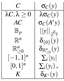
A number of functions can be built up from support functions. For example, any norm can be defined as the support function of a closed convex set (namely, the unit ball of the associated dual norm). Table 2 contains common examples.

3.5 Summary

Figure 3 provides a concise summary of some of the most important ideas we have presented in this section. In the summary, we ignore necessary technical conditions, but we emphasize that all the applications of convex analysis in this paper refer to and demonstrate the relevant technical con-ditions. We believe this summary will be useful, especially to readers unfamiliar with the abstract theory of convex functions and conjugacy.

C σC(y)

λC,λ_≥0 λσC(y)

AC σC(Aty)

Bp ||y|| p p−1

Rn δ{0}(y)

Rn_≥0 δRn

≤0(y)

[₋1,1]n _∑ i|yi|

[0,1]n _∑ i(yi)+

K δK◦(y)

Table 2: Support functions for common convex sets. C and C0are arbitrary non-empty closed con-vex sets. K is an arbitrary non-empty closed concon-vex cone. A is an arbitrary matrix.

Summary of Key Convex Analysis Concepts • (Fenchel-Legendre Conjugate) f∗(z) =sup_y{ytz−f(y)_}. • (Biconjugation) f∗∗= f .

• (Fenchel-Young Theorem) f(y)₋ytz+f∗(z)_≥0, and z_∈∂f(y)_⇔y_∈∂f∗(z)_⇔ f(y)₋

yt_z+f∗_{(z) =0.}

• (Fenchel Duality) The minimizer of f(y) +g(y)satisfies f(y)₋ytz+f∗(z) = 0

g(y) +ytz+g∗(₋z) = 0

for some z which also minimizes f∗(z) +g∗(₋z).

• (Auxiliary Parameters: h0(y) =infuh(y,u)) h0∗(z) =h∗(z,0).

• (Infimal Convolutions:(f?g)(y) =infy0{f(y−y0) +g(y0)})(f?g)∗=f∗+g∗.

• (Indicator and Support Functions)δC(y) =

0 y_∈C

∞ y_∈/C, andσC(z) =supy∈Cy

t_z.δ∗

C=σC.

If C is a vector space,δ∗_C=δ_C⊥.

4. Tikhonov Regularization

We now specialize the general theory of Fenchel duality to the inductive learning scenario.

Definition 19 (loss functions and regularization) A loss function is any closed convex function v :R→(∞,∞], which is bounded below and finite at 0.

A regularization is any closed convex function R :Rn→R≥0, such that R(0) =0.

Typically, a loss function, vi, represents the penalty for a value mismatching some prescribed

value or set of values (e.g., vi(yi) = (yi−Yi)2), while a regularization represents a measure of

non-smoothness among a set of values y1, . . . ,yn.

Clearly, regularizations and loss functions are closed under addition. We can also show that the conjugates of regularizations and loss functions are, respectively, regularizations and loss functions.

Lemma 20 If v is a loss function, then v∗ is a loss function. If R is a regularization, then R∗ is a regularization.

Proof Since v∗and R∗are closed and convex, we need only show that v∗is bounded below and finite at 0 and that R∗(z)_≥0 with R∗(0) =0.

v is bounded below, so v∗(0) =₋infyv(y)is finite. v(0) =−infzv∗(z)is finite, so v∗is bounded

below.

Since R(0) =₋infzR∗(z) =0, R∗is non-negative and R∗(0) =−infyR(y) =0.

As a consequence, regularizations and losses are closed under infimal convolution.

The following lemma shows that if the loss function can be decomposed over data points, then its conjugate can likewise be decomposed.

Lemma 21 Let V :Rn→(₋∞,∞]be given by V(y) =∑_in₌₁vi(yi)for loss functions vi. Then V∗(z) =

∑n

i=1v∗i(zi).

Proof A direct consequence of the definition,

V∗(z) = sup

y

(

ytz−

∑

i

vi(yi)

)

=

∑

i

sup

yi {

yizi−vi(yi)}

=

∑

i

v∗_i(zi).

We are now able to state the main theorem that we will use to study regularization problems.

Theorem 22 (regression Fenchel duality) Let R : Rn → R≥0 be a regularization and V(y) = ∑n

i=1vi(yi)for loss functions vi:R→R. If 0∈int(dom R−dom V)or 0∈int(dom R∗+dom V∗)

then

inf

y,z{R(y) +V(y) +R

∗_{(z) +V}∗_(−z)}=0

with all minimizers y,z satisfying the complementarity equations:

R(y)₋ytz+R∗(z) = 0 (13)

vi(yi) +yizi+v∗i(−zi) = 0. (14)

loss dual loss optimality condition v(y) v∗(₋z) v(y) +yz+v∗(₋z) =0 f(Y₋y) f∗(z)₋zY f(Y₋y) + (Y₋y)(₋z) +f∗(z) =0 f(1−yY) f∗ _Yz−z

Y f(1−yY) + (1−yY)− z Y +f∗

z Y =0 1 2y 2 1 2z

2 _y+z=0

|y_| δ_[−1,1](z) _|y_|+yz=0,z_∈[₋1,1] (y)+ δ[−1,0](z) (y)++yz=0,z∈[−1,0]

1

2(y)2+ δR≤0(z) +

1

2z2 (y)++z=0,z≤0 (_|y_{| −}ε)+ δ[−1,1](z) +ε|z|

|y_{| ≥}ε z+sign(y) =0 |y_{| ≤}ε z_∈[₋1,1]

1 2(Y−y)

2 1

2z

2_{−zY y+z=Y}

|Y₋y_| δ_[−1,1](z)−zY |Y−y|= (Y−y)z,z∈[−1,1]

|1₋yY_| δ[−1,1] Yz

−Yz |1−yY|= (1−yY) z Y,

z

Y ∈[−1,1]

(1₋yY)+ δ[0,1] Yz

−z

Y (1−yY)+= (1−yY) z Y,

z

Y ∈[0,1]

1

2(1−yY) 2

+ δR≥0

z Y +1 2 z2

Y2 −_Yz (1−yY)+=_Yz,_Yz ≥0

(_|Y₋y_{| −}ε)+ δ[−1,1](z) +ε|z| −zY

|Y₋y_{| ≥}ε z=sign(Y₋y) |Y₋y_{| ≤}ε z_∈[₋1,1]

log(1+exp(₋yY)) δ_[0,1] z Y

+ z Ylog

z

Y+ 1= (1+exp(−yY)) z Y

1_−Yzlog 1_−Yz

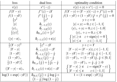
Table 3: A list of common loss functions and their local optimality conditions. Note that we are considering v∗(₋z), not v∗(z). Also note that some of the loss functions can be further simplified under the assumption Y_{∈ {−}1,1_}.

We identify the yi as values taken by the learned function, scored by vi, and the function values are

penalized by R(y). Equation 13 is a complementarity equation in 2n variables. Equation 14 is n independent complementarity equations in 2 variables. If R and viare differentiable these equations

are equivalent to z=∇R(y)and₋zi=_dydvi(yi).

4.1 Loss Functions

Table 3 recapitulates many of the loss functions seen in practice. In this paper, we deal exclusively with pointwise losses, so Table 3 is in terms of a single regression value y and a single training value Y with subscripts omitted.

The derivations in Table 3 can all be obtained without much effort from identities and defini-tions previously stated and earlier derivadefini-tions in the table. It is helpful to observe that many loss functions can be expressed in terms of infimal convolutions of simple functions. For example, (y)+=σ[0,1](y) = (| · |?δR≤0)(y)and(|y| −ε)+= (| · |?δ[−ε,ε])(y).

It should be noted that these derivations can be checked graphically, since the losses are func-tions of a single variable. For example, Figure 4 shows a graph of (1₋y)+, the well-known

(

1

,

0

)

(

0

,

1

)

h

(

y

) =

4

(

1

₋

y

)

/

5

h

(

y

) = (

1

₋

y

)

/

3

y

(

1

₋

y

)

+

Figure 4: The graph of(1₋y)+with a couple supporting hyperplanes.

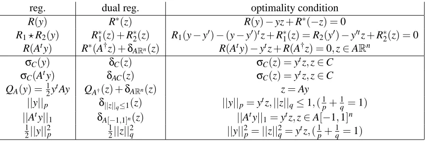
4.2 Regularization Functions

By Lemma 20, if R1,R2:Rn→[0,∞]are regularizations, then R1+R2and R1?R2are, which gives two ways of building more complicated regularizations out of simpler ones. The basic building blocks of regularizations are indicator functions, support functions, and quadratic forms. The iden-tities to keep in mind areσ_C∗ =δC, Q∗A=QA−1 for non-singular A, and R1?R₂= (R∗₁+R∗₂)∗(with

appropriate conditions from Theorem 15).

We might think of sums of regularizations as adding further penalties on the regression values, as R_≤R+R0. On the other hand, infimal convolutions add slack, R_≥R?R0. Since these two operations are conjugates of each other, it is clear that any additional restriction in the primal results in extra freedom in the dual and vice versa.

5. Regularization in Reproducing Kernel Hilbert Spaces

reg. dual reg. optimality condition R(y) R∗(z) R(y)₋yz+R∗(₋z) =0

R1?R2(y) R∗1(z) +R∗2(z) R1(y−y0)−(y−y0)tz+R∗1(z) =R2(y0)−y0tz+R∗2(z) =0 R(Aty) R∗(A†z) +δARn(z) R(Aty)−ytz+R(A†z) =0,z∈ARn

σC(y) δC(z) σC(z) =ytz,z∈C

σC(Aty) δAC(z) σC(z) =ytz,z∈C

QA(y) = 1₂ytAy QA†(z) +δ_ARn(z) z=Ay

||y_||p δ_||z_||q≤1(z) ||y||p=y t_z,||z||

q≤1,(1_p+1_q=1)

||Aty_||1 δA[−1,1]n(z) ||Aty||₁=ytz,z∈A[−1,1]n

1 2||y||

2

p 12||z|| 2

q ||y||2p=||z||2q=ytz,(1p+

1

q =1)

Table 4: Common regularization choices.

5.1 Optimality Conditions for RKHS Regularization

Recall that the “standard” approach in machine learning is to start with a Tikhonov regularization problem over an RKHS (2), to invoke the representer theorem to show that the solution can be expressed as a collection of coefficients (3), and to write optimization problems in terms of these coefficients. We start with a mathematical program in terms of the yi, using a regularization QK−1

(with K symmetric, positive definite); in this framework, we are able to state general optimality conditions and derive a very clean form of the representer theorem.

Specialized to the RKHS case, we are considering primal problems of the form

inf

y∈Rn

1 2λy

t_K−1_y+V(y)

,

where we have made the target labels Yiimplicit in V . The associated dual problem is

inf

z∈Rn

1 2λ

−1_zt_Kz+V∗_(z)

.

Equation 13 specializes to

1 2λy

t_K−1_y

−ytz+1 2λ

−1_zt_{Kz = 0}

1 2(y−λ

−1_Kz)t_(λK−1_y

−z) = 0.

and thus we obtain the optimality conditions z=λK−1y (or y=λ−1_{Kz). This demonstrates that} whenever we are performing regularization in an RKHS, the optimal y values at the training points can be obtained by multiplying the optimal dual variables z byλ−1K, for any convex loss function. 5.2 RKHS Regularization Examples

In RKHS regularization, we have a regularizer R(y) =λQ_K−1(y), with conjugate R∗(z) =λ−1Q_K(z),

5.2.1 REGULARIZEDLEASTSQUARES

The square loss is given by v(yi) = 1₂(Yi−yi)2. Although it is listed in Table 3, we derive the dual

loss here, for pedagogical purposes:

v∗(₋z) =sup

y0 {−

y0z₋1 2(y

0_−Y)2_}.

We see that v∗(₋z)is quadratic in y0, and we can find the sup by taking the derivative:

∂v∗

∂y0 =−z+ (Y−y0).

Setting the derivative to 0, we obtain y=Y₋z, and substituting, we see that

v∗(₋z) =₋zY+1 2z

2_.

The optimality equation v(yi) +yizi+v∗(zi)reduces to y+z=Y , so (13) and (14) become

yi+zi = Yi

λ−1_{Kz = y.} Combined,

y+λK−1y=λ−1_Kz+z=Y, leading to the standard regularized least squares formulation.

5.2.2 UNBIASEDSVM

The support vector machine arises from the combination of RKHS regularization and the hinge loss v(y) = (1−yY)+.The dual of the hinge loss, v∗(−z) =δ[0,1](Yz)−

z

Y, is most easily derived using a

graphical approach (see Figure 4), but it can also be derived directly. Regularizing in an RKHS, we have the primal and dual problems:

inf

y_∈Rn

(

1 2λy

t_K−1_y+

∑

i

(1₋yiYi)+ )

inf

z_∈Rn

(

1 2λ

−1_zt_Kz+

∑

δ[0,1]

zi

Yi

−zi

Yi

)

.

We see how theδfunction in the dual loss provides the well-known “box constraints” in the SVM dual.

Given v(y),v∗(₋z), it is also straightforward to derive the optimality condition

(1₋yY)+= (1−yY)

z

Y and

z

A case analysis on the sign of(1−yY)yields

(1₋yiYi)<0 ⇐⇒

zi

Yi

=0

(1₋yiYi) =0 ⇐⇒

zi

Yi ∈

[0,1]

(1₋yiYi)>0 ⇐⇒

zi

Yi

=1.

With the regularization condition y=λ−1_{Kz, we have derived the KKT conditions for the SVM. To} obtain a more “standard” formulation, we could introduce variablesαi≡_Yizi, c=λ−1z, eliminating

y from the system (in favor of z andα), and introducing a “regularization constant” C= ₂1_λ. In this section, we have derived an “unbiased” SVM. In practice, the SVM usually includes an unregularized bias term b. We show how to handle the bias term b in Section 9.1.

6. L1 Regularizations

Tikhonov regularization in a reproducing kernel Hilbert space is the most common form of regu-larization in practice, and has a number of mathematical properties which make it especially nice. In particular, the representer theorem makes RKHS regularization essentially the only case where we can start with a problem of optimizing an infinite-dimensional function in a function space, and obtain a finite-dimensional representation.5 Nevertheless, other regularizations may be of interest. In these cases, we are generally forced to assume a priori that the functions we are looking for are coefficients in some finite dimensional space.

6.1 1-norm Support Vector Machines

As a consequence of the use of the hinge loss, support vector machines yield a sparse solution— points which live outside the margin have c=z=0. Nevertheless, because all points which are errors or live inside the margin are support vectors, in noisy problems, one generally finds that at least a constant fraction of the examples (lower-bounded by the Bayes error rate) are support vectors. Instead of using RKHS regularization, we can a priori choose a finite-dimensional function space of expansion coefficients of kernel functions around the training points y=∑_iK(x,xi)ci, and

regularize_||c_||1. If we combine this idea with the hinge loss, we obtain the 1-norm support vector machine (Zhu et al., 2003).

We consider R(y) =_||K−1y||1. If we use the hinge loss (or any other piecewise linear loss function), the resulting mathematical optimization problem is a linear program. The dual regularizer is R∗(z) =δ_K−1_[−1,1]n(z). As usual, we can combine primal and dual regularizers with primal and

dual loss functions. Note that in these formulations, the formula c=λ−1_{z does not hold: if we} solved a problem in y and z, we would need to then solve c=K−1y to obtain c. In practice, we expect that algorithms based directly on c are probably the most useful.

6.2 Sparse Approximation and Support Vector Regression

In Girosi (1998), an “equivalence” between a certain sparse approximation problem and a modified form of SVM regression is developed. In slightly simplified form, the equivalence is quite easy to derive.

We begin by considering the sparse approximation problem. We are given noiseless samples {(X1,Y1), . . . ,(Xn,Yn)}from a target function ft which is assumed to live in an RKHS

H

find a function which is a coefficient expansion around the data points: f(x) =∑_iK(x,xi),ci. The

goal is to minimize the distance between ftand f(x)in the RKHS norm,6while maintaining sparsity of the coefficient representation c:

inf

c_∈Rn

1 2||f

t_−f||2

H +ε||c||1

=1 2||f

t_||2 H +_cinf_∈Rn

1 2c

t_Kc−Yt_c+ε||c||

1

.

where we used basic properties of RKHS and the assumption that ft(x)_∈

H

which lie outside a tube. Girosi instead considers a “hard margin” variant, where points are required to lie inside the tube. His primal problem is:

inf

y_∈Rn

λQ_K−1(y) +δ_[−ε_,ε_]n(Y−y) .

The dual to the “hard loss” v(yi) =δ[−ε,ε](Yi−yi)is given by

v∗(₋zi) = sup y0_i {−

y0_izi−δ[Yi−ε,Yi+ε](y0i)}

= max_{−(Yi−ε)zi,−(Yi+ε)zi}

= ₋Yizi+ε|zi|.

Therefore, the dual problem is

inf

z_∈Rn

λ₋₁

QK(z)−Ytz+ε||z||1 =λ· inf

z_∈Rn

QK(λ−1z)−Yt(λ−1z) +ε||λ−1z||1 .

We see that the sparse approximation variant and the support vector regression variant have optimal values that differ by a constant 1_2||ft_||2_H and a positive multiplierλ, with c=λ−1_{z. The sparsity} control parameterεbecomes the width of the allowed tube in the regression problem. This makes sense: as we increaseε, we get more sparsity, but our predicted y values must become less tightly constrained in order to achieve that sparsity.7

6. In earlier treatments of sparse decomposition (such as Chen et al., 1995) the goal was to minimize functional distance in L2rather thanH; this distance (of course) needed to be approximated empirically.