Taking One for the Team: Is collective action more responsive to ecological change?
Charles Sims* ([email protected]) is a Faculty Fellow at the Howard H. Baker Jr. Center for Public Policy and an assistant professor in the Department of Economics at the University of Tennessee, 1640 Cumberland Ave, Knoxville, TN 37996.
David Finnoff ([email protected]) is an associate professor in the Department of Economics and Finance, 1000 E. University Avenue, University of Wyoming, Laramie, WY 82071. Jason F. Shogren ([email protected]) is Stroock Professor of Natural Resource Conservation and Management in the Department of Economics and Finance, 1000 E. University Avenue, University of Wyoming, Laramie, WY 82071.
* corresponding author
Abstract
Debate persists around the timing of risk reduction strategies for large-scale ecological change for three reasons: risks are difficult to predict, they involve irreversibilities, and they impact multiple jurisdictions. The combination of these three factors creates a general class of filterable spatial-dynamic externalities (FSDE) in which one person’s risk reduction investments reduce or
filter undesirable events experienced by others and underestimates the option value placed on being able to respond to new information about the consequences of ecological change. By focusing on the optimal intervention decision, we illustrate how and when the opposing forces created by an FSDE will lead to a divergence in private and collective risk reduction strategies. We use bioinvasions as our motivating example. The bioinvasion first hits one jurisdiction, and that jurisdiction’s risk reduction investment reduces the risk faced by all other jurisdiction. We find that efforts to internalize the full benefits of risk reduction investments may have unintended consequences on the responsiveness of environmental policy. There is a social welfare gain from asking the first jurisdiction to delay a risk reduction investment to internalize the option values of all at-risk jurisdictions.
2 1. Introduction
Governments react to the risks posed by large scale ecological change (e.g., climate change, biodiversity loss) by making long-term investments in mitigation or adaptation or both. Defining cost-effective risk reduction investment strategies, however, remains a challenge because ecological risks (the likelihood and severity of an unfavorable ecological event) are not localized—they spread over multiple jurisdictions with little incentive to address impacts outside a decision maker’s area of concern. In a static endogenous risk world, in which private actions either filter or transfer risk, a social planner may call for more or less mitigation accordingly relative to private actions (see Shogren and Crocker 1991).1 However, ecological risks are also long term – the stream of damages occurs over long time horizons, which limits how well we can predict the benefit of mitigation (avoided future damage) and the magnitude of these
externalities. In a dynamic world, efforts to reduce ecological risk are risky investments since costs are incurred in exchange for uncertain payoffs. The riskiness of these investments has not been considered in a filterable or transferable risk setting, limiting our understanding of the optimal timing of risk-reduction strategies.
Herein we address this gap by focusing on the timing of a private and collective
mitigation investment in a dynamic endogenous risk framework. Like any risky investment, the efficiency of risk reduction strategies hinges on timing (Arrow and Fisher 1974, Henry 1974). If ecological change turns out to be larger than expected, a policy maker will regret a strategy of inaction that generated irreversible damage. This provides an argument for a more immediate
1 For instance, a filterable extenality will arise when efforts to control pests or invasive species by an indivudal
3
response (Chichilnisky and Heal 1993, Fisher and Hanemann 1993). Likewise, if ecological change turns out to be smaller than expected, the policymaker will regret the strategy of immediate action since slower-than-expected ecological change constitutes bad news for the return on risk reduction investments (Pindyck 2007). This focus on downside risk provides an argument against immediate action.2 These push-pull incentives on the timing decision are linked since high levels of ecological risk necessarily imply more risky investments (Sims, Finnoff et al. 2016). When investments must be made to reduce ecological risk, policymakers value flexibility and this value is the policy’s option value. The existence of an option value means it pays to keep options open.
It is well-known that option values influence the timing of risk-reduction investments (Dixit and Pindyck 1994). Our model is novel in that it considers this timing decision in the context of a prevalent class of filterable spatial-dynamic externalities (FSDE). An FSDE accounts for how undesirable ecological events are filtered over time and space. Failure to internalize the FSDE ignores ecological risk faced by other jurisdictions and makes the investment appear less risky.3 A collective perspective does not ignore the FSDE and pools ecological risk across all potentially impacted jurisdictions to internalize external effects of risk reduction investments. But since pooling ecological risk implies pooling investment risk, a
2 The focus on downside risk in our model is an environmental analog of Bernanke’s “bad news principle”
(Bernanke 1983) and arises due to the combination of uncertainty in the benefits of a risk reduction strategy and the irreversible investment needed to initiate the risk reduction strategy. A focus on downside risk may also arise if
returns are nonnormally distributed and decision makers are particularly averse to deviations below a benchmark return (Shah and Ando 2015).
3
4
collective investment is guided by a risk-reward tradeoff. A collective investment in mitigation has a higher expected return but is also more likely to generate a return that is lower than expected. As a result, the option value associated with a collective mitigation investment is larger than the option value associated with an individual mitigation investment. Little is known about how this risk-reward tradeoff influences the timing of collective action in response to ecological change. This is because the literature on optimally timing responses to ecological change has focused primarily on a single decision maker.4 We consider both private and collective timing of risk reduction investments given the potential for multiple decision-making agents.
As a motivating example we consider the case in which a bioinvasion first affects one jurisdiction before moving on to neighboring jurisdictions. Jurisdictions can make a one-time sunk cost investment in mitigation that slows the bioinvasion. Three reasons prompt our choice. First, bioinvasions are widely accepted as one of the leading contributors of biodiversity loss (Didham, Tylianakis et al. 2005) and are increasing worldwide, impacting agriculture, forestry, fisheries, and ecosystem services.5 Second, bioinvasions are a prime example of the conflicting incentives for risk reduction investment (Sims and Finnoff 2013). Early investments in invasive species control avoid potentially irreversible change to ecosystems. But avoiding investments in species predicted to become invasive, that in fact would not have, is desirable (Smith, Lonsdale et al. 1999, Williamson 1999) and the information needed to make this determination is valuable.
4
Socially optimal investment decisions have been considered for environmental pollutants (Pindyck 2000, Pindyck 2002, Saphores 2004), biodiversity loss (Kolstad 1996), agricultural pest species (Saphores 2000), and invasive species (Saphores and Shogren 2005, Marten and Moore 2011). Sims and Finnoff (2012) introduce spatial considerations for a generic environmental problem.
5 See Lodge (2001) and Mack et al. (2000). Impacts to agricultural production are demonstrated in Archer and
5
Third, the results speak to an ongoing and well-publicized debate among ecologists concerning the need for urgency in response to bioinvasions (Davis, Chew et al. 2011, Simberloff 2011).
With a focus on optimal intervention policy, our model has two key results: (1) a private individual’s immediate investment is less than the social optimum given he has no incentive to consider the expected damage to all his neighbors, but (2) we find no definitive results emerge about the timing of investment. The reason for the ambiguity is that a tension exists between the desire to respond to ecological change in a timely manner and the need to keep policy options open given the future uncertainty surrounding the consequences of the invasion. Individual agents and society view this tension differently because of the FSDE. Society must address all risk posed by ecological change (more proof a response is needed) but it also experiences more regret from premature action (a larger burden of proof is needed to initiate a response). Since the FSDE filters both ecological and investment risk, society may prefer to delay a mitigation
6
Due to the differences between private and collective option values, collective actions may not be more responsive to ecological change. This suggests that efforts to internalize the full risk of ecological damage may have unintended consequences on the timing of the policy response. This result runs counter to the “precautionary principle”—which asks regulators to not let uncertainty about future impacts delay their investments in reducing the risk of serious or irreversible damage (Farrow 2004). Here, precaution focuses on the possibility of regretting inaction that caused irreversible ecological change. Previous arguments for prudence against the precautionary principle have been based on future learning(Ulph and Ulph 1997, Gollier, Jullien et al. 2000, Asano 2010) and tradeoffs between mitigation and control (Athanassoglou and Xepapadeas 2012). We provide an alternative justification based on flexibility values. A decision maker may regret inaction that caused irreversible change and regret action that commits funds to a mitigation strategy that is not warranted. Our model weighs these countervailing sources of precaution over time (Fenichel, Tsao et al. 2008). When these countervailing sources of precaution are allowed to play out with multiple decision makers, private mitigation decisions in accordance with the precautionary principle underestimate the value society places on being able to respond to new information about the consequences of ecological change.
Our results also inform the relationship between the value of information and adaptive management in a specific setting (Walters and Hilborn 1978, Walters 1986). The option value in our analysis can be interpreted both as a value of flexibility or as a value of information
7
value of new information about ecological change is lost (or significantly reduced) once the policy maker acts. In this setting, the value of information creates an incentive to delay mitigation. Under an adaptive management paradigm, new information about the nature of ecological change is also valuable and mitigation is conducted as a deliberate experiment. But in this setting, mitigation can be continuously adjusted in response to new information so that the value of information incentivizes more immediate or more aggressive action in an effort to elicit information.
2. An illustrative example
We begin with a motivating example to illustrate the basic structure of the model. In Figure 1, assume a bioinvasion spreads along a corridor of space from an origin at a rate given by the weight of the dashed arrow.6 While current invaded area A0 is known with certainty, future invaded area is unknown.7 The corridor consists of a succession of contiguous jurisdictions (i.e. private landholdings, countries or states) in which the bioinvasion is sequentially advancing over the areas. The total area of the corridor 𝐴̅ is divided into N
jurisdictions with the area of jurisdiction 𝑖 = 1, … , 𝑁 given by 𝐴̅𝑖 = 𝐴̅ − ∑𝑖−1𝑛=1𝐴̅𝑛. Following Kolstad and Ulph (2011) and others, each jurisdiction is controlled by a distinct, risk-neutral agent (i.e., landowner or government official). Damages are a function of the invaded area implying current damages are known with certainty but future damages are unknown. To reduce expected damages, each agent can choose if and when to invest in a mitigation strategy that
6
For optimal control of a damaging species spreading in two dimensions see Epanchin-Niell and Wilen (2012) and Aadland, Sims et al. (2015).
7 For some bioinvasions, the current extent of the invasion is unknown and investments to control the spread must be
8
would slow the spread of the invasion. Figure 1 depicts a hypothetical corridor of uniformly shaped jurisdictions where mitigation implemented at ti slows the spread to a rate given by the
weight of the white arrow.
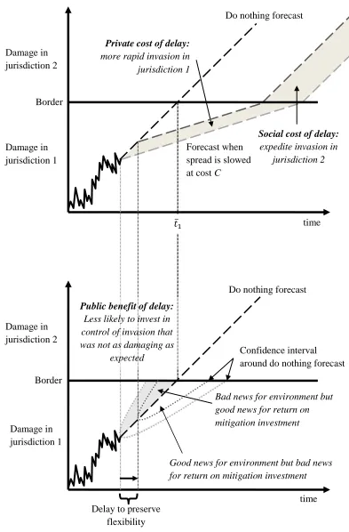
Figure 2 shows the motivation for the mitigation decision. In both panels the horizontal axis is time following the start of the invasion, the vertical axis the damages from invasion. Jurisdiction 1 extends from the origin to the border, jurisdiction 2 above the border. The solid black line represents the evolution of invasion damages up to the current time. The positively sloped black dashed line represents the expected damages if there is no mitigation (do nothing) and the invasion progresses at the current rate first through jurisdiction 1 and then jurisdiction 2 and beyond. The confidence intervals around the do nothing forecast are shown in the lower panel. The decision facing jurisdiction 1 is when (at what time) to invest in a policy that would slow the spread at some cost C. Jurisdiction 1 evaluates the choice to mitigate at each instant in time by forming a forecast for how bad the invasion would be if left uncontrolled. If the
9
also a cost to delay since the invasion spreads at a faster rate for a longer period of time which increases the discounted damages from invasion in jurisdiction 1 (a private cost) and hastens invasion to other areas (a social cost).
A private decision ignores the cost of obtaining new information associated with expediting the invasion in jurisdiction 2. This implies that private decisions will lag collective decisions. But the value of the information gained by delay is smaller for a private decision since the repercussions of the decision (expected damages prevented) are lower. This implies that private decisions preempt collective decisions. To assess which of these countervailing incentives dominates, we assume future invaded area evolves according to a geometric Brownian motion (GBM) process:
𝑑𝐴 = 𝑟0𝐴𝑑𝑡 + 𝑠𝐴𝑑𝑧 (1)
where r0 is the rate of invasion absent any intervention, s is the standard deviation coefficient, and dz is the increment of a standard Weiner process.8 Larger values for r0 imply faster invasion corresponding to a more mobile species. Likewise larger values of s correspond to a larger amount of uncertainty in future invaded area. This uncertainty arises due to natural variability such as changes in temperature and precipitation. The generality of GBM is attractive but it also has two particularly desirable properties for bioinvasions. First, since complete eradication is unlikely (Dahlsten, Garcia et al. 1989), it rules out non-positive levels of invaded area.9 Second
8 Equation (1) implies future invaded area is a log-normally distributed random variable with expected value 𝐴 0𝑒𝑟
0𝑡
and variance 𝐴02𝑒2𝑟0𝑡(𝑒𝑠2𝑡− 1).
9 A lower absorbing barrier on the stochastic process could be included to allow for species extinction. In aspatial
10
it allows the invasion to accelerate as invaded area grows as often observed with human
interactions.10 But it also implies that invaded area is unbounded. To restrict invaded area to a finite level, equation (1) is subjected to an upper barrier 𝐴̅ which represents a physical boundary (e.g., mountain range, body of water) or a perceived boundary such as county, state, or federal borders (Sims and Finnoff 2012).
Assume each agent’s damage is a convex function of the invaded area within their jurisdiction:
𝐷𝑖(𝐴) =
{
0
𝛾 [𝐴(𝑡) − ∑ 𝐴̅𝑛 𝑖−1
𝑛=1 ]
𝜃
𝐷̅𝑖
𝑖𝑓 𝐴(𝑡) ≤ ∑ 𝐴̅𝑛 𝑖−1
𝑛=1
𝑖𝑓 ∑ 𝐴̅𝑛 𝑖−1
𝑛=1 < 𝐴(𝑡) < ∑ 𝐴̅𝑛 𝑖
𝑛=1
𝑖𝑓 𝐴(𝑡) ≥ ∑𝑖 𝐴̅𝑛 𝑛=1
(2)
where θ ≥ 1, γ > 0, and 𝐷̅𝑖 = 𝛾𝐴̅𝑖𝜃.11 While current damage is known with certainty, future
damage is unknown due to uncertainty surrounding future invaded area. Through Ito calculus, we derive a GBM process for damage in each jurisdiction:
𝑑𝐷𝑖 = 𝛼0𝐷
𝑖𝑑𝑡 + 𝜎𝐷𝑖𝑑𝑧 (3)
subject to the upper barrier 𝐷̅𝑖 where 𝛼0 = 𝜃𝑟0+12𝜃(𝜃 − 1)𝑠2 and 𝜎 = 𝜃𝑠.
An agent’s mitigation strategy instantly reduces the rate of invasion in their jurisdiction from r0 to 𝑟𝑝, a change that affects the invasion in jurisdiction i and when the invasion reaches all other jurisdictions. To reflect the irreversible nature of environmental damage 𝑟𝑝 ≥ 0 which
10
For instance, invasive species spread increases exponentially in the presence of long-distance, human-mediated dispersal (Shigesada, Kawasaki et al. 1995). Long-distance dispersal is the rule rather than the exception for invasive species (Hengeveld 1989).
11
ensures expected damages will never decline: 𝛼𝑝 = 𝜃𝑟𝑝+12𝜃(𝜃 − 1)𝑠2 ≥ 0. There are few cases in which invasive species control has caused the invaded area to decline. One can achieve local eradication, but rarely do you see total invaded area shrink. Like any investment, the mitigation strategy imposes an irreversible flow of costs on the agent in jurisdiction i. For instance, a mitigation strategy by a state or country may prohibit trade in commodities known to harbor foreign invading organisms. The present value of the expected flow of sunk costs
associated with this mitigation strategy at time of investment depends on the extent of jurisdiction i and the spread rate reduction, denoted by 𝐶𝑖 = 𝑐𝐴̅𝑖(𝑟0− 𝑟𝑝)2.12
We restrict our attention to the case in which the magnitude of the mitigation investment is fixed but the timing of this investment can be chosen optimally. Alternatively, the agent in jurisdiction i may choose the magnitude of investment 𝑟𝑖𝑝 but must invest immediately. In this setting, the presence of a FSDE will cause the agent in jurisdiction i to engage in less mitigation (see Appendix) which confirms previous results (Shogren and Crocker 1991). By focusing on a given investment we highlight how the FSDE impacts the timing of mitigation which reveals a less intuitive result.
3. Timing of mitigation investments
Our model focuses on the timing of mitigation given uncertainty. We determine the optimal time to mitigate for private and collective decision making by 1) evaluating the decision
12 Our cost function is consistent with control strategies that do not depend on the current size of the invaded area
12
to mitigate at all instants in time, and 2) comparing this choice to not mitigating at that instant. For instance, at each instant in time the agent in jurisdiction i decides whether a mitigation strategy that reduces the rate of invasion to 𝑟𝑝 should be adopted immediately given the
uncertainty in future invaded area. Immediate mitigation lowers the growth in expected damages in jurisdiction i but incurs costs Ci. Otherwise mitigation is postponed until the next instant in
time in which the agent is faced with the same binary choice concerning mitigation. Mitigation becomes the preferred alternative when current damage reaches or exceeds a critical threshold. We find the optimal time to adopt this mitigation strategy by comparing the current level of damage to the critical damage threshold in each jurisdiction.
From the perspective of the individual jurisdiction, the present value of expected damage and mitigation costs in jurisdiction 1 over an infinite horizon, when mitigation is adopted at 𝑡1 is:
𝑊1 = 𝐸0[ ∫ 𝐷1(𝛼0)𝑒−𝜌𝑡𝑑𝑡 𝑡1
0
⏟ 𝑒𝑥𝑝𝑒𝑐𝑡𝑒𝑑 𝑝𝑟𝑒𝑠𝑒𝑛𝑡 𝑣𝑎𝑙𝑢𝑒
𝑜𝑓 𝑑𝑎𝑚𝑎𝑔𝑒 𝑏𝑒𝑓𝑜𝑟𝑒 𝑚𝑖𝑡𝑖𝑔𝑎𝑡𝑖𝑜𝑛 𝑖𝑛
𝑗𝑢𝑟𝑖𝑠𝑑𝑖𝑐𝑡𝑖𝑜𝑛 1
+ ∫ 𝐷1(𝛼𝑝)𝑒−𝜌𝑡𝑑𝑡 𝑡̅1
𝑡1
⏟ 𝑒𝑥𝑝𝑒𝑐𝑡𝑒𝑑 𝑝𝑟𝑒𝑠𝑒𝑛𝑡 𝑣𝑎𝑙𝑢𝑒 𝑜𝑓 𝑑𝑎𝑚𝑎𝑔𝑒 𝑎𝑓𝑡𝑒𝑟 𝑚𝑖𝑡𝑖𝑔𝑎𝑡𝑖𝑜𝑛 𝑖𝑛 𝑗𝑢𝑟𝑖𝑠𝑑𝑖𝑐𝑡𝑖𝑜𝑛 1 𝑏𝑢𝑡 𝑏𝑒𝑓𝑜𝑟𝑒
𝑏𝑒𝑐𝑜𝑚𝑖𝑛𝑔 𝑓𝑢𝑙𝑙𝑦 𝑖𝑛𝑣𝑎𝑑𝑒𝑑
+ 𝐷̅1 𝜌 𝑒−𝜌𝑡̅1 ⏟ 𝑒𝑥𝑝𝑒𝑐𝑡𝑒𝑑 𝑝𝑟𝑒𝑠𝑒𝑛𝑡 𝑣𝑎𝑙𝑢𝑒 𝑜𝑓 𝑐𝑜𝑛𝑠𝑡𝑎𝑛𝑡 𝑓𝑙𝑜𝑤 𝑑𝑎𝑚𝑎𝑔𝑒 𝑤ℎ𝑒𝑛 𝑗𝑢𝑟𝑖𝑠𝑑𝑖𝑐𝑡𝑖𝑜𝑛 1
𝑖𝑠 𝑓𝑢𝑙𝑙𝑦 𝑖𝑛𝑣𝑎𝑑𝑒𝑑
+ 𝐶⏟ 1𝑒−𝜌𝑡1 𝑒𝑥𝑝𝑒𝑐𝑡𝑒𝑑 𝑝𝑟𝑒𝑠𝑒𝑛𝑡 𝑣𝑎𝑙𝑢𝑒 𝑜𝑓 𝑚𝑖𝑡𝑖𝑔𝑎𝑡𝑖𝑜𝑛 𝑠𝑡𝑟𝑎𝑡𝑒𝑔𝑦 𝑖𝑛𝑐𝑢𝑟𝑟𝑒𝑑
𝑎𝑡 𝑡1
] (4)
where 𝐸0 is the expectation operator based on information available to agent 1 at 𝑡 = 0 and ρ is the discount rate.13 Following mitigation at 𝑡1, the invasion continues to spread at rate 𝑟𝑝 until 𝑡̅1 = 𝑡1 + 1
𝛼𝑝−1 2𝜎2
ln ( 𝐷̅1
𝐷1(𝑡1)) at which point jurisdiction 1 is fully invaded. With nothing left to
13 In the dynamic programming approach we employ, the discount rate is exogenously determined and should equal
13
save, agent 1 terminates his mitigation effort and the damage-causing process returns to its original rate of spread r0 as it passes into the next area (jurisdiction 2).
The mitigation decision in all other jurisdictions 𝑗 = 2, … , 𝑁 is similar. Once a
jurisdiction becomes invaded, the same mitigation strategy can be adopted in that jurisdiction. If adopted at 𝑡 = 𝑡𝑗, the present value of expected damage and mitigation costs in jurisdiction j
(when initially invaded at 𝑡̅𝑗−1) over an infinite horizon is
𝑊𝑗= 𝐸𝑡̅𝑗−1[∫ 𝐷𝑡𝑗 𝑗(𝛼0)𝑒−𝜌𝑡𝑑𝑡 𝑡̅𝑗−1
⏟
𝑒𝑥𝑝𝑒𝑐𝑡𝑒𝑑 𝑝𝑟𝑒𝑠𝑒𝑛𝑡 𝑣𝑎𝑙𝑢𝑒 𝑜𝑓 𝑑𝑎𝑚𝑎𝑔𝑒 𝑏𝑒𝑓𝑜𝑟𝑒 𝑚𝑖𝑡𝑖𝑔𝑎𝑡𝑖𝑜𝑛 𝑖𝑛
𝑗𝑢𝑟𝑖𝑠𝑑𝑖𝑐𝑡𝑖𝑜𝑛 𝑗
+ ∫ 𝐷𝑡̅𝑗 𝑗(𝛼𝑝)𝑒−𝜌𝑡𝑑𝑡 𝑡𝑗
⏟
𝑒𝑥𝑝𝑒𝑐𝑡𝑒𝑑 𝑝𝑟𝑒𝑠𝑒𝑛𝑡 𝑣𝑎𝑙𝑢𝑒 𝑜𝑓 𝑑𝑎𝑚𝑎𝑔𝑒 𝑎𝑓𝑡𝑒𝑟 𝑚𝑖𝑡𝑖𝑔𝑎𝑡𝑖𝑜𝑛 𝑖𝑛 𝑗𝑢𝑟𝑖𝑠𝑑𝑖𝑐𝑡𝑖𝑜𝑛 𝑗 𝑏𝑢𝑡 𝑏𝑒𝑓𝑜𝑟𝑒
𝑏𝑒𝑐𝑜𝑚𝑖𝑛𝑔 𝑓𝑢𝑙𝑙𝑦 𝑖𝑛𝑣𝑎𝑑𝑒𝑑
+ 𝐷̅𝑗 𝜌 𝑒−𝜌𝑡̅𝑗 ⏟
𝑒𝑥𝑝𝑒𝑐𝑡𝑒𝑑 𝑝𝑟𝑒𝑠𝑒𝑛𝑡 𝑣𝑎𝑙𝑢𝑒 𝑜𝑓 𝑐𝑜𝑛𝑠𝑡𝑎𝑛𝑡 𝑓𝑙𝑜𝑤 𝑑𝑎𝑚𝑎𝑔𝑒 𝑤ℎ𝑒𝑛 𝑗𝑢𝑟𝑖𝑠𝑖𝑑𝑐𝑖𝑡𝑜𝑛 𝑗
𝑖𝑠 𝑓𝑢𝑙𝑙𝑦 𝑖𝑛𝑣𝑎𝑑𝑒𝑑
+ 𝐶𝑗𝑒−𝜌𝑡𝑗
⏟ 𝑒𝑥𝑝𝑒𝑐𝑡𝑒𝑑 𝑝𝑟𝑒𝑠𝑒𝑛𝑡 𝑣𝑎𝑙𝑢𝑒 𝑜𝑓 𝑚𝑖𝑡𝑖𝑔𝑎𝑡𝑖𝑜𝑛 𝑠𝑡𝑟𝑎𝑡𝑒𝑔𝑦 𝑖𝑛𝑐𝑢𝑟𝑟𝑒𝑑
𝑎𝑡 𝑡𝑗
] (5)
where 𝐸𝑡̅𝑗−1 is the expectation operator based on information available when jurisdiction j
initially becomes invaded, 𝐷̅𝑗 is the upper bound on damage experienced by the agent in jurisdiction j, and 𝑡̅𝑗 = 𝑡𝑗+𝛼𝑝−11
2𝜎2
ln ( 𝐷̅𝑗
𝐷𝑗(𝑡𝑗)) is the expected time until jurisdiction j is fully invaded. The social, or multi-jurisdictional expected present value of damage and costs experienced over all jurisdictions is 𝑊 = 𝑊1+ ∑𝑁𝑗=2𝑊𝑗𝑒−𝜌𝑡̅𝑗−1 given the sequential nature of
the invasion.
14
information values results in a private optimum damage threshold 𝐷1′. Initiating mitigation at this point in the invasion 𝐴1′ minimizes 𝑊1.
If agent 1 were to be compensated for this delay through market mechanisms or Coasean-like bargaining, the FSDE could be internalized. This would increase agent 1’s private value of mitigation and a social optimum damage threshold 𝐷1∗ (or invaded area threshold 𝐴1∗) could be achieved. If all other agents were also similarly compensated, social costs over all jurisdictions 𝑊 would be minimized. Since the FSDE filters benefits and costs of agent 1’s private mitigation investment, it is unclear whether 𝐴1∗ < 𝐴1′ or 𝐴1∗ > 𝐴1′. If the filtered benefit of agent 1’s
mitigation outweighs the cost, all other agents would prefer agent 1 act sooner (𝐴1∗ < 𝐴1′). By acting sooner, agent 1 must forfeit flexibility but all other agent’s damages are delayed further into the future. If the filtered costs outweigh the benefits, however, all other agents would prefer agent 1 take a loss for the team and delay mitigation (𝐴1∗ > 𝐴1′). Taking one for the team leads
to additional damages for agent 1 but also preserves management flexibility for the collective.
In what follows we first characterize the socially optimal timing of the mitigation decision in jurisdiction 1 from the perspective of all jurisdictions. We then derive the FSDE by contrasting the collective decision in jurisdiction 1 with that of the private decision.
3.1. Collective timing
A collective of agents shares the cost of mitigation on each parcel but considers the
15
chooses mitigation strategies across the entire invaded area (i.e., in jurisdictions 1 through N).14 For simplicity we focus on the first jurisdiction and only compare the collective and agent 1 mitigation strategies. The same comparison can be made for mitigation strategies in all jurisdictions. The sequential nature of the analysis does not alter the general results as the actions of “downstream” other agents do not affect “upstream” agents.
The collective chooses to initiate the mitigation strategy in jurisdiction 1 when the current level of damage in that region reaches the collective damage threshold 𝐷1∗. The collective
damage threshold in jurisdiction 1 follows from two boundary conditions. The first boundary condition is the value matching condition: 𝑊1𝐶(𝐷1∗) = 𝑊1𝐼(𝐷1∗). This requires the payoff from postponing mitigation to equal the payoff from immediate mitigation. The collective
continuation value 𝑊1𝐶 represents the payoff from postponing the mitigation investment: the discounted expected damage from doing nothing in jurisdiction 1 and the value from being able to respond to new information about the invasion (the flexibility or option value). The flexibility value is lost once the investment is made since economic commitments prevent any policy adjustments in response to new information. This economic irreversibility makes the option value conditional on the collective delaying the mitigation strategy. The implementation value 𝑊1𝐼 represents the discounted expected damage from immediate mitigation in jurisdiction 1,
taking into account the consequences on all agents. The second boundary condition is known as the smooth pasting condition: 𝑊1,𝐷𝐶 (𝐷1∗) = 𝑊1,𝐷𝐼 (𝐷1∗) where subscript D indicates partial
derivatives with respect to current damage. This condition balances payoffs from postponing
14 This provides a consistent comparison to the privately optimal case in which N mitigation investments will also be
16
and implementing mitigation at the margin. Smooth pasting requires the continuation and implementation marginal values are balanced at 𝐷1∗.
Following a dynamic programming approach outlined in Sims and Finnoff (2012), we first solve for the continuation value in jurisdiction 1:
𝑊1𝐶 = 𝐷1
(𝜌 − 𝛼0)− 𝑍10𝐷1𝜀
0
+ ∑ 𝑊𝑗𝑒
−𝜌( 1
𝛼0−1
2𝜎2 ln(𝐷𝐷̅1
1)+∑ 𝑡̅𝑛 𝑗−1 𝑛=2 )
𝑁
𝑗=2
+ 𝜂𝐷1𝜀0 (6)
where η < 0 is an unknown constant of integration, 𝑍10 = 𝛼 0𝐷̅
1
𝜌(𝜌−𝛼0)𝐷̅1𝜀0, and 𝜀
0 = (1 2−
𝛼0
𝜎2) +
√(𝛼𝜎02−12)2+2𝜌𝜎2 is the positive root of the fundamental quadratic associated with the Bellman
equation.15 The first two terms capture the private consequences of doing nothing. The first term in (6) represents the discounted expected damage over an infinite spatial horizon (ignoring jurisdiction 1’s boundaries). The second term captures how the size of the jurisdiction limits the expected discounted damage experienced in jurisdiction 1. The repercussion of doing nothing to all other agents (third term in equation 6) is the present value of more immediate invasion in all other jurisdictions (given by 1
𝛼0−1 2𝜎2
ln (𝐷̅1
𝐷1) + ∑ 𝑡̅𝑛
𝑗−1
𝑛=2 ) if damage is currently D1 and nothing is done.
The collective repercussion of doing nothing is the preservation of the collective flexibility or option value represented by the term 𝜂𝐷1𝜀
0
. This option value is nonpositive as it
15 Equation (6) assumes 𝐷̅
1 is an upper absorbing barrier which implies damage is permanent. With the upper bound
17
reduces damages. Delaying mitigation allows more irreversible damage in jurisdiction 1, but the delay also preserves society’s ability to respond to new information on the severity of the
invasion. A mitigating investment eliminates the ability to respond to this new information thereby eliminating its value. The option value captures this additional opportunity cost of investing in mitigation.
The implementation value is equal to the expected present value of immediate mitigation in jurisdiction 1 from a collective viewpoint is:
𝑊1𝐼 = 𝐷1
(𝜌 − 𝛼𝑝)− 𝑍1𝑝𝐷1𝜀
𝑝
+ 𝐶1+ ∑ 𝑊𝑗𝑒
−𝜌( 1
𝛼𝑝−1
2𝜎2 ln(𝐷𝐷̅1
1)+∑ 𝑡̅𝑛 𝑗−1 𝑛=2 )
𝑁
𝑗=2
(7)
where 𝑍1𝑝 = 𝛼 𝑝𝐷̅
1
𝜌(𝜌−𝛼𝑝)𝐷̅1𝜀𝑝 and 𝜀
𝑝 = (1 2−
𝛼𝑝
𝜎2) + √(
𝛼𝑝
𝜎2 −
1 2)
2
+2𝜌𝜎2 > 𝜀0. The consequences on
jurisdiction 1 of immediate mitigation are given by the first three terms in (7). The first and second terms measure the (bounded) expected damages in jurisdiction 1 following mitigation, and 𝐶1 is the cost of mitigation in jurisdiction 1. The effect of immediate mitigation on all other agents (the fourth term in 7) is again driven by 1
𝛼𝑝−1 2𝜎2
ln (𝐷̅1
𝐷1) + ∑ 𝑡̅𝑛
𝑗−1
𝑛=2 which is the expected
time it takes for jurisdiction j to become invaded if mitigation in jurisdiction 1 is undertaken immediately.
The collective optimal timing of the mitigation investment in jurisdiction 1 is given by value matching and smooth pasting boundary conditions. These conditions jointly result in an optimality condition we express as a benefit cost ratio:16
18 𝐷1∗ 𝛼0 − 𝛼𝑝
(𝜌 − 𝛼0)(𝜌 − 𝛼𝑝) −(𝜀
𝑝− 𝜀0) (𝜀0− 1) 𝑍1𝑝𝐷1∗𝜀
𝑝
+𝜀0X − 𝐷1∗Δ (𝜀0− 1) 𝜀0
(𝜀0− 1) 𝐶1
= 1 (8)
where
𝑋 = ∑ 𝑊𝑗𝑒−𝜌(∑ 𝑡̅𝑛
𝑗−1 𝑛=2 )
[ 𝑒
−𝜌( 1
𝛼0−1
2𝜎2 ln(𝐷̅1
𝐷1∗)) − 𝑒
−𝜌( 1
𝛼𝑝−1
2𝜎2 ln(𝐷̅1
𝐷1∗))
] 𝑁
𝑗=2
> 0 (9)
is the value of delaying the time all other agents are invaded and:
Δ = 𝜕X
𝜕𝐷1∗ = ∑
𝜌𝑊𝑗𝑒−𝜌(∑𝑗−1𝑛=2𝑡̅𝑛) 𝐷1∗
[ 𝑒
−𝜌( 1
𝛼0−1
2𝜎2 ln(𝐷̅1
𝐷1∗))
𝛼0−1 2 𝜎2
−𝑒
−𝜌( 1
𝛼𝑝−1
2𝜎2 ln(𝐷̅1
𝐷1∗))
𝛼𝑝−1 2 𝜎2
] 𝑁
𝑗=2
(10)
is the change in this value due to delaying mitigation in jurisdiction 1. The solution for 𝐷1∗ in (8) serves as the critical damage threshold that must be reached to justify a collectively chosen mitigation investment in jurisdiction 1.
3.2. Individual timing
19
agent 1 optimally invests in mitigation when damage reaches or exceeds 𝐷1′ which ensures the following benefit cost ratio is equal to 1:17
𝐷1′ 𝛼0− 𝛼𝑝
(𝜌 − 𝛼0)(𝜌 − 𝛼𝑝) −(𝜀
𝑝− 𝜀0) (𝜀0− 1) 𝑍1𝑃𝐷1′ 𝜀
𝑝
𝜀0 (𝜀0− 1) 𝐶1
= 1 (11)
Comparing (8) to (11) we find that the benefit of mitigation under collective timing includes the additional term 𝜀
0X−𝐷 1∗Δ
(𝜀0−1) which captures the effect of the FSDE on agent 1’s mitigation decision. When 𝜀
0X−𝐷 1∗Δ
(𝜀0−1) > 0, the benefit of collectively timed mitigation is greater and will occur before individual mitigation. When 𝜀
0X−𝐷 1∗Δ
(𝜀0−1) < 0, collectively timed mitigation will be delayed longer than individual efforts.
3.3 Countervailing factors
The FSDE at any point in the invasion is the change in all other agent’s discounted damages due to agent 1’s mitigation decision and is given by X > 0. From (9), the externality is increasing in other agent’s expected damage and the number of other agents N. The effect of all other parameters depends upon the relative magnitude of the parameters of the problem. The change in the FSDE due to delaying mitigation is Δ, which may be ⋛ 0. The delay in mitigation results in a more immediate time that all other agents expect to become invaded. With damages being realized at an earlier point in time, X is larger. However, delaying mitigation also places a downward pressure on X as the mitigation strategy operates for a shorter amount of time. The
20
two effects are countervailing, which obfuscates exactly how delaying mitigation affects the FSDE.
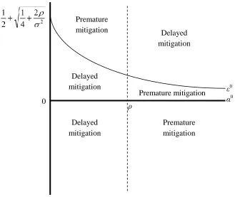
The inability to sign Δ prevents definitive statements about the influence of a FSDE on the timing of agent 1’s mitigation investment. Figure 3 shows the potential outcomes. With the standard assumption of relatively high discount rate in comparison to the drift rate of spread, 𝜌 > 𝛼0, we find 𝜀0 > 1. Here, the FSDE causes agent 1 to sub-optimally delay mitigation (𝐷1′ > 𝐷1∗) if Δ < 𝜀
0
𝐷1∗X. This inequality can also be rewritten as
𝜕X 𝜕𝐷1∗
𝐷1∗
𝑋 < 𝜀0 where the left-hand
side can be interpreted as the elasticity of the externality with respect to a delay in mitigation investments. When this elasticity is less than 𝜀0 we know the individual will delay longer than collectively optimal, 𝐷1′ > 𝐷1∗. But if this elasticity is greater than 𝜀0 (Δ > 𝜀
0
𝐷1∗X or 𝜕X 𝜕𝐷1∗
𝐷1∗
𝑋 > 𝜀 0),
the FSDE results in premature mitigation by agent 1 such that 𝐷1′ < 𝐷1∗. Now society prefers agent 1 to delay mitigation efforts because society values flexibility more than the individual – take a loss for the team. Because the collective mitigation investment yields larger expected benefits, the collective values information about future ecological change more than the private individual.18 As an alternative interpretation, society’s mitigation investment is more risky than the individual’s since pooling ecological risk also pools investment risk. Regardless of the interpretation, this result runs against intuition and demonstrates the importance of this elasticity in understanding how a FSDE impacts the timing of mitigation investments. When 𝜌 < 𝛼0 and
18 This result does not imply that the uncertainty associated with mitigation on other parcels has been reduced. The
21
𝜀0 < 1, the inequalities above are reversed and premature mitigation by agent 1 arises when 𝜕X
𝜕𝐷1∗
𝐷1∗
𝑋 < 𝜀 0.19
This counterintuitive result is explained by countervailing effects of the FSDE on the benefit and opportunity cost of mitigation investments. Internalizing the FSDE unambiguously increases the reduction in expected damages from mitigation investments in jurisdiction 1. By considering the expected present value of all other agent’s damage, 𝑊1𝐶 increases by more than 𝑊1𝐼 which raises the benefit of implementing the mitigation strategy by X. This creates a
downward pressure on 𝐷1∗. As shown in the Appendix, the effect of the FSDE on the opportunity cost of mitigation (seen through changes in the option value) is unclear. If a 1% increase in 𝐷1∗ (a delay in mitigation) increases the externality by less than 1% (Δ < 𝐷X
1∗ or
𝜕X 𝜕𝐷1∗
𝐷1∗
𝑋 < 1),
internalizing the FSDE decreases the opportunity cost of mitigation. The externality’s impact on the benefit and opportunity cost of mitigation reinforce one another creating a downward
pressure on 𝐷1∗. The FSDE is primarily filtering damages and causes agent 1 to underinvest in bioinvasion mitigation which manifests as a sub-optimal delay in mitigation. In contrast, if a 1% increase in 𝐷1∗ increases the externality by more than 1% (Δ > 𝐷X
1∗ or
𝜕X 𝜕𝐷1∗
𝐷1∗
𝑋 > 1), internalizing the
FSDE increases the opportunity cost of collective mitigation creating an opposing upward pressure on 𝐷1∗. In this case the filtering of flexibility values causes agent 1 to under invest in acquiring information which manifests as a sub-optimally hasty investment in mitigation.
19 With an upper bound on damage, the traditional assumption 𝜌 > 𝛼0 is not needed to ensure finite expected
22
These results run against the general idea of the “precautionary principle”. Recall the precautionary principle asks regulators to not wait to make current investments in risk reduction just because they are uncertain of future damages (Farrow 2004). Our model provides an economic justification for prudence against the precautionary principle. If we follow the precautionary principle in our model, we forfeit the flexibility values of all other agents. There is a social economic value for the initially impacted individual to delay control and absorb the loss to preserve the flexibility that other agent’s value. The other agents will only value flexibility for the mitigation investment in jurisdiction 1 if all agents share the cost of the mitigation investment. In a setting in which collective action only arises through a mutually agreeable division of the mitigation cost, the flexibility values of other agents must be considered to ensure that efforts to reduce ecological risk do not also reduce the economic values that other agent’s hold.
4. Illustrative Example with Two Agents
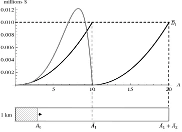
To investigate the likelihood of these counterintuitive results, we consider a hypothetical example with 2 agents depicted in Figure 4, which could represent any pair of agents and
jurisdictions. Let damage be quadratic in invaded area (θ = 2) and the initial km2 of invaded area cause $100 in damage (γ = 0.0001). Now assume if left unchecked, the invasion will spread at a rate of 3% per year (r0 = 0.03) with a variability of 2% around this trend (s = 0.02). A mitigating investment would slow this rate of spread to 1% annually (𝑟𝑝 = 0.01). Also assume total
23
$10,000. Agent 1’s initially invaded area is 3 km2. The mitigation strategy requires a $20,000 investment (c = 5). Finally, assume each agent operates with an 8% discount rate (ρ = 0.08).
The FSDE initially increases as the invasion spreads through jurisdiction 1 (see Figure 4). This arises because a delay in mitigation causes agent 2 to be invaded sooner. Once invaded area reaches 8 km2, the FSDE begins to shrink as mitigation becomes less effective at delaying
invasion in jurisdiction 2 due to the short amount of time the mitigation strategy is in effect. Once the invasion has spread fully through jurisdiction 1, agent 1’s decision no longer affects when agent 2 becomes invaded, driving the FSDE to 0. A mitigation investment in jurisdiction 2 does not create a FSDE since the boundary of jurisdiction 2 physically stops the invasion.
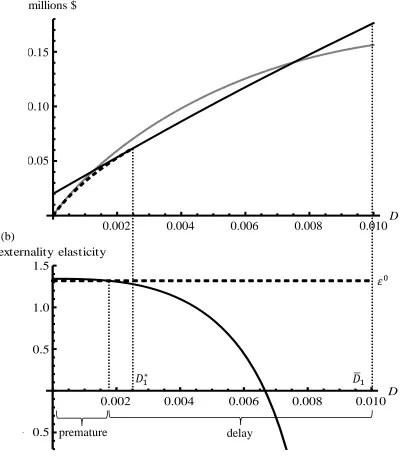
Figure 5a presents the payoffs from collectively timed mitigation investments. Internalizing the FSDE adds to the discounted expected damage avoided through mitigation. This increases the benefit of mitigation and creates a downward pressure on 𝐷1∗. Internalizing the FSDE also increases the option value associated with the mitigation investment, creating an upward pressure on 𝐷1∗. We determine which of these two opposing forces dominates by
comparing the externality elasticity and the positive root of the fundamental quadratic associated with the Bellman equation (see Figure 5b). The externality elasticity (𝜕X
𝜕𝐷1∗
𝐷1∗
𝑋) is 1.28 at the time
of collective mitigation. Since 𝜀0 = 1.32 > 1.28, we know the FSDE will lead to delayed mitigation: 𝐷1′ > 𝐷1∗. If the FSDE is internalized, a mitigating investment in jurisdiction 1 would occur approximately 1 month earlier when damage reaches 𝐷1∗ = $2,459 or when jurisdiction 1 is approximately 50% invaded.
24
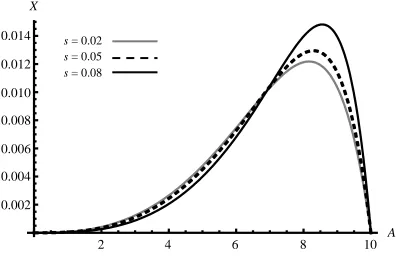
that these results are robust to changes in most parameters with the exception of uncertainty. From Figure 6 we see more uncertainty may either increase or decrease the magnitude of the FSDE depending on the current invaded area. We can find general results on the effect of uncertainty if we focus on the externality elasticity (see Figure 7). With little uncertainty (s = 0.001), the externality elasticity always lies below 𝜀0 ensuring the FSDE causes a delay in mitigation. Here the externality primarily filters damages since there is little value provided by remaining flexible for such a predictable ecological change. With a sufficient degree of
uncertainty, the FSDE can cause agent 1 to prematurely invest in mitigation. Agent 1’s hasty mitigation investment delays agents 2’s exposure to damage but also prevents future adjustments to the mitigation policy in response to new information. As part of the collective, agent 2 would prefer that agent 1 delay mitigation to preserve the flexibility to respond to new information about the invasion on jurisdiction 1. At the margin, this flexibility is more valuable than the expected delay in damage.
25
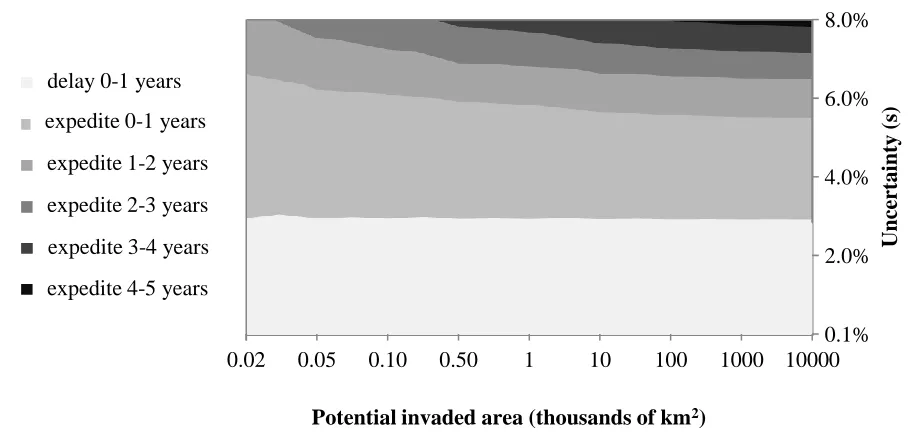
early. When jurisdiction 1 is much smaller than jurisdiction 2 (area at risk is 100,000 km2), the FSDE will cause agent 1 to invest in mitigation 4 to 5 years too early. This premature action lowers expected damages but also lowers social welfare by prematurely terminating the option value of all other agents. While the precautionary principle may seem defensible when
uncertainty is great and the area at risk is large, this is precisely the setting where the value of flexibility is most undervalued by private decision makers.
5. Internalizing a filterable spatial-dynamic externality
We now explore how to internalize the FSDE in our numerical example. Matching individual and social optimums requires that agent 2 pay agent 1 to adjust his timing of
mitigation. To ensure incentive compatibility, this payment takes place at the socially optimal time of mitigation 𝑡1∗. At this point in time, the payment is a random variable since it depends on the time jurisdiction 2 becomes invaded which is itself a random variable. Let 𝜏 = 𝑡̅1(𝐷1′) be the expected time jurisdiction 2 becomes invaded if agent 1 acts in his own best interest. The
following payment structure can be used to internalize the FSDE:
𝑝𝑎𝑦𝑚𝑒𝑛𝑡 = {𝛿𝐸𝑡1∗[𝑡̅1− 𝜏] 𝑖𝑓 𝐷1
′ > 𝐷 1∗
𝛿𝐸𝑡1∗[𝜏 − 𝑡̅1] 𝑖𝑓 𝐷1′ < 𝐷1∗ (12)
26
total payment received from agent 2. The optimal payment to agent 1 from 2 that internalizes the FSDE is:20
𝛿 = 𝜀0𝑋 − 𝐷1∗Δ
[𝜀0(𝑡̅
1(𝐷1∗) − 𝑡̅1(𝐷1′)) + 𝛼 0− 𝛼𝑝
(𝛼0−1
2 𝜎2) (𝛼𝑝−12 𝜎2) ]
(13)
This payment is positive since 𝐷1′ > 𝐷1∗ requires 𝜀0𝑋 − 𝐷1∗Δ > 0.
When 𝐷1′ < 𝐷1∗, agent 2 pays agent 1 for each unit of time that the arrival of damage in jurisdiction 2 is expedited. The longer agent 1 delays mitigation beyond the individual optimum, the smaller 𝑡̅1, and the greater the total payment received from agent 2. In either case, if agent 1 continues to ignore agent 2’s discounted expected damage, 𝑡̅1= 𝑡̅1(𝐷1′) and the payment is 0. A
similar procedure can be used to find 𝛿.
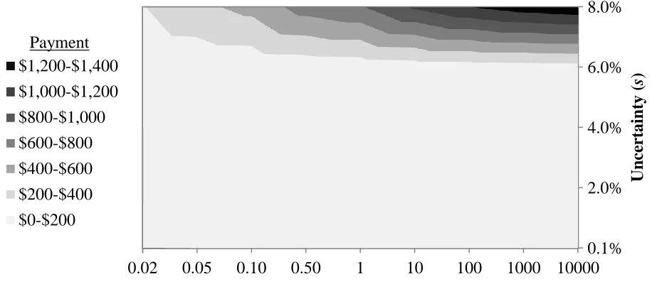
In the numerical example with little uncertainty (s = 0.02) and a small area at risk (𝐴̅ = 20), the FSDE’s two countervailing impacts are offset. As a result, agent 2 would only need to pay agent 1 $1.55 to incorporate the externality. The payment is needed to internalize physical benefits that accrue to other agents. As shown in Figure 9, with more uncertainty and a larger area at risk, the size of the payment between the two agents increases. When s is less than 6%, the payment between the two agents needed to incorporate the FSDE and maximize social welfare will be less than $200 regardless of the area at risk. In contrast, when uncertainty is larger (s > 8%) and the area at risk is larger than 5,000 km2, the payment between the two agents to incorporate the FSDE exceeds $1,000. Now the payment acts to compensate agent 1 for preserving the flexibility of collective action – taking a loss for the team. In contrast to payments
27
that internalize physical benefits, payments that internalize the value of flexibility encourage more delayed investments in mitigation.
6. Conclusions
Cost-effective risk reduction investments in response to large-scale ecological change remain elusive due to the inability to accurately predict when, where, and to whom damages will occur. To maximize the welfare of all at-risk agents (inclusive of their option values), society must weigh a tradeoff between immediate risk reduction investments that effectively limit expected damages and delayed strategies that allow us to respond to new information about the consequences of ecological change. To help clarify this tradeoff, this paper presents a model of private mitigation investment in response to uncertain ecological change.
Using bioinvasions as an example, we show the timing of individual policy decisions are biased by a filterable spatial-dynamic externality that impacts the benefit of mitigation
investments (in terms of reduced expected discounted damage) and the cost of mitigation investments (in terms of lower value on the ability to respond to new information about ecological change). When the process of ecological change is more certain, the first effect dominates and the FSDE causes an individual to delay mitigation beyond what would be chosen by society as a whole. When ecological change is more uncertain, the presence of the FSDE encourages premature mitigation. In these instances, there is an economic value for the initially impacted agents to delay responses to ecological change so society can respond to new
28
the context of environmental policy, this result is consistent with the information acquisition literature. For example, Choi (1991) shows that when technology adoption leads to network externalities, there may be too much early adoption of technologies compared to the social optimum.
These results have particular implications for responding to bioinvasion risk. Since bioinvasion control is a public good (Perrings, Williamson et al. 2002), individual control decisions will fall short of collective action (Wilen 2007, Richards, Ellsworth et al. 2010, Fenichel, Richards et al. 2014, Kovacs, Haight et al. 2014). Most efforts to align individual and collective incentives have centered on Pigovian taxes and Coasean bargaining solutions designed to encourage more intensive control actions by the individual decision maker. When control actions involve economic commitments (e.g., sunk costs or spraying treatments of a fixed size) and the future benefits of those actions are uncertain, corrective mechanisms may be needed to delay control actions by the individual decision maker when the ability to respond to new information about the severity of the bioinvasion is more valuable to society.
29
agreements creates an incentive to delay. With these countervailing irreversibilities, our model suggests that international environmental agreements that include nations that are currently impacted by ecological change could be adopted before more comprehensive agreements that include nations that will be impacted in the future.
To provide insightful analytic results, our model abstracts from several factors that will be investigated in future work. While the uncertainty of future ecological change is a central part of most policy debates, mitigation effectiveness and the current extent of the invasion may also be uncertain. In an adaptive management setting, these types of uncertainty may generate more immediate or more aggressive mitigation in an effort to reduce these uncertainties. In our model, where policy makers are unable to act on this information, considering these types of uncertainty would likely strengthen our results. Both types of uncertainty would add to the uncertainty in discounted stream of benefits associated with the mitigation investment and would reinforce the option value that drives the “take one for the team” result. Our current model assumes
completely irreversible environmental damage and mitigation investments. We think it would be insightful to more intermediate forms of irreversibility. For example, cases in which damages only become irreversible when an unknown critical threshold is reached and where mitigation decisions are adjusted periodically. This would allow for the possibility that the maximum level of damage could be avoided if decision makers respond in a timely manner.
Appendix
30
Assume agent 1 invests in mitigation immediately but may choose the magnitude of the investment rp. The optimal magnitude of investment by agent 1 is:
min 𝑟𝑝 {𝑊
𝐼(𝐷
10, 𝑟𝑝)} = 𝐷10 (𝜌 − 𝛼𝑝)−
𝛼𝑝𝐷̅ 1 𝜌(𝜌 − 𝛼𝑝)𝐷̅
1𝜀
𝑝𝐷10𝜀
𝑝
+ 𝐶1 (𝐴. 1)
The first-order condition for this problem implicitly defines the private optimum mitigation investment 𝑟𝑝′(𝐷10):
𝜃𝐷10 (𝜌 − 𝛼𝑝′)2−
𝜃𝐷̅1 (𝜌 − 𝛼𝑝′)2(
𝐷10 𝐷̅1)
𝜀𝑝′
[1 − (ln𝐷1 0
𝐷̅1) Ω] = 2𝐶1′
𝑟0− 𝑟𝑝′ (𝐴. 2)
where Ω =𝛼
𝑝′(𝜌−𝛼𝑝′)
𝜎2𝜌 [ 1 − 𝛼𝑝′ 𝜎2− 1 2
√(𝛼𝑝𝜎2′−12)
2
+2𝜌𝜎2 ]
> 0 and 𝐶1′ = 𝑐𝐴̅1(𝑟0− 𝑟𝑝′)2 . The left (right) hand
side is the marginal cost (benefit) of choosing less mitigation or higher rp. The size of agent 1’s spatial jurisdiction influences the amount of mitigation through the second term on the left-hand side of (A.2).
The optimal amount of mitigation in jurisdiction 1 by the collective is:
min
𝑟𝑝 {𝑊 𝐼(𝐷
10, 𝑟𝑝)} =
𝐷10
(𝜌 − 𝛼𝑝)−
𝛼𝑝𝐷̅ 1
𝜌(𝜌 − 𝛼𝑝)𝐷̅ 1𝜀
𝑝𝐷10𝜀 𝑝
+ 𝐶1+ ∑ 𝑊𝑗𝑒
−𝜌( 1
𝛼𝑝 −12𝜎2ln(
𝐷̅1
𝐷10)+∑𝑗−1𝑛=2𝑡̅𝑛) 𝑁
𝑗=2
(𝐴. 3)
The first-order condition implicitly defines the social optimum amount of mitigation 𝑟𝑝∗(𝐷10):
𝜃𝐷10 (𝜌 − 𝛼𝑝∗)2−
𝜃𝐷̅1 (𝜌 − 𝛼𝑝∗)2(
𝐷10 𝐷̅1)
𝜀𝑝∗
[1 − (ln𝐷1 0
31 +∑ 𝑊𝑗𝑒
−𝜌(∑𝑗−1𝑛=2𝑡̅𝑛)
𝑁
𝑗=2 𝜌𝜃
(𝛼𝑝∗−1 2 𝜎2)
2 ln (
𝐷̅1 𝐷10) 𝑒
−𝜌( 1
𝛼𝑝∗−1
2𝜎2 ln(𝐷̅1
𝐷10))
= 2𝐶1 ∗
𝑟0− 𝑟𝑝∗ (𝐴. 4)
Once again the left (right) hand side is the marginal cost (benefit) of less mitigation or higher rp. Compared to (A.2), internalizing the FSDE leads to an additional cost of less mitigation. This is arises because less mitigation allows the invasion to spread faster after the mitigation investment decreasing the time until agent 2’s damage is incurred.
It is straightforward to show 𝑟𝑝′> 𝑟𝑝∗. Equation (A.2) can be rewritten as:
𝜃𝐷10 = 2𝐶1′(𝜌 − 𝛼𝑝′) 2
𝑟0− 𝑟𝑝′ + 𝜃𝐷̅1( 𝐷10 𝐷̅1)
𝜀𝑝′
[1 − (ln𝐷1 0
𝐷̅1) Ω
′] (𝐴. 5)
Equation (A.4) can be rewritten as:
𝜃𝐷10 = 2𝐶1∗(𝜌 − 𝛼𝑝∗)2
𝑟0− 𝑟𝑝∗ + 𝜃𝐷̅1( 𝐷10 𝐷̅1)
𝜀𝑝∗
[1 − (ln𝐷10 𝐷̅1) Ω∗]
−(𝜌 − 𝛼
𝑝∗)2∑ 𝑊
𝑗𝑒−𝜌(∑ 𝑡̅𝑛
𝑗−1 𝑛=2 )
𝑁
𝑗=2 𝜌𝜃
(𝛼𝑝∗−1 2 𝜎2)
2 ln (
𝐷̅1 𝐷10) 𝑒
−𝜌( 1
𝛼𝑝∗−1
2𝜎2 ln(𝐷̅1
𝐷10))
(𝐴. 6)
Setting these equal to one another
2𝐶1′(𝜌 − 𝛼𝑝′)2
𝑟0− 𝑟𝑝′ + 𝜃𝐷̅1(
𝐷10
𝐷̅1)
𝜀𝑝′
[1 − (ln𝐷10
𝐷̅1) Ω′] −
2𝐶1∗(𝜌 − 𝛼𝑝∗)2
𝑟0− 𝑟𝑝∗ − 𝜃𝐷̅1(
𝐷10
𝐷̅1)
𝜀𝑝∗
[1 − (ln𝐷10 𝐷̅1) Ω∗]
= −(𝜌 − 𝛼
𝑝∗)2∑ 𝑊
𝑗𝑒−𝜌(∑ 𝑡̅𝑛 𝑗−1 𝑛=2 ) 𝑁
𝑗=2 𝜌𝜃
(𝛼𝑝∗−1
2 𝜎2)
2 ln (
𝐷̅1 𝐷10) 𝑒
−𝜌( 1
𝛼𝑝∗−12𝜎2ln( 𝐷̅1 𝐷10))
32 Since the right-hand side of (A.7) is negative we know:
2𝐶1∗(𝜌 − 𝛼𝑝∗)2
𝑟0− 𝑟𝑝∗ + 𝜃𝐷̅ ( 𝐷10 𝐷̅1)
𝜀𝑝∗
[1 − (ln𝐷1 0
𝐷̅1) Ω∗]
>2𝐶1
′(𝜌 − 𝛼𝑝′)2
𝑟0− 𝑟𝑝′ + 𝜃𝐷̅1( 𝐷10 𝐷̅1)
𝜀𝑝′
[1 − (ln𝐷1 0
𝐷̅1) Ω′] (A. 8)
which implies 𝑟𝑝′> 𝑟𝑝∗ since the left- and right- hand sides of the above expression are
functionally equivalent. The FSDE causes agent 1 to engage in less mitigation. This is intuitive and confirms previous results (Shogren and Crocker 1991).
Derivation of collective and individual timing threshold conditions
The value matching condition is
𝜂𝐷1∗𝜀0 + 𝐷1∗
(𝜌 − 𝛼0)− 𝑍10𝐷1∗𝜀
0
+ ∑ 𝑊𝑗𝑒
−𝜌( 1
𝛼0−1
2𝜎2 ln(𝐷𝐷̅1
1∗)+∑ 𝑡̅𝑛 𝑗−1 𝑛=2 )
𝑁
𝑗=2
= 𝐶1+ 𝐷1∗
(𝜌 − 𝛼𝑝)− 𝑍1𝑝𝐷1∗𝜀
𝑝
+ ∑ 𝑊𝑗𝑒
−𝜌( 1
𝛼𝑝−1
2𝜎2 ln(𝐷𝐷̅1
1∗)+∑ 𝑡̅𝑛 𝑗−1 𝑛=2 )
𝑁
𝑗=2
(𝐴. 9)
The smooth pasting condition is
𝜀0𝜂𝐷 1∗𝜀
0−1
+ 1
(𝜌 − 𝛼0)− 𝜀0𝑍10𝐷1∗𝜀
0−1
+𝜌 ∑ 𝑊𝑗𝑒
−𝜌(∑𝑗−1𝑛=2𝑡̅𝑛)
𝑁 𝑗=2
𝐷1∗
𝑒
−𝜌( 1
𝛼0−1
2𝜎2 ln(𝐷𝐷̅1
1∗))
33
= 1
(𝜌 − 𝛼𝑝)− 𝜀𝑝𝑍1𝑝𝐷1∗𝜀
𝑝−1
+𝜌 ∑ 𝑊𝑗𝑒
−𝜌(∑𝑗−1𝑛=2𝑡̅𝑛)
𝑁 𝑗=2
𝐷1∗
𝑒
−𝜌( 1
𝛼𝑝−1
2𝜎2 ln(𝐷𝐷̅1
1∗))
𝛼𝑝−1 2 𝜎2
(𝐴. 10)
Combining (A.9) and (A.10) we find
𝜀0 𝐷1∗
[
∑ 𝑊𝑗𝑒−𝜌(∑ 𝑡̅𝑛
𝑗−1 𝑛=2 ) 𝑁 𝑗=2 [ 𝑒 −𝜌( 1
𝛼𝑝−1
2𝜎2 ln(𝐷𝐷̅1
1∗)) − 𝑒
−𝜌( 1
𝛼0−1
2𝜎2 ln(𝐷𝐷̅1
1∗))
] +𝐶1 + 𝐷1∗
(𝜌 − 𝛼𝑝)− 𝑍1𝑝𝐷1∗𝜀
𝑝
+ 𝑍10𝐷 1∗𝜀
0
− 𝐷1∗
(𝜌 − 𝛼0) ]
+ 1
(𝜌 − 𝛼0)− 𝜀0𝑍10𝐷1∗𝜀
0−1
+𝜌 ∑ 𝑊𝑗𝑒
−𝜌(∑𝑗−1𝑛=2𝑡̅𝑛)
𝑁 𝑗=2
𝐷1∗
𝑒
−𝜌( 1
𝛼0−1
2𝜎2 ln(𝐷𝐷̅1
1∗))
𝛼0−1 2 𝜎2
= 1
(𝜌 − 𝛼𝑝)− 𝜀𝑝𝑍1𝑝𝐷1∗𝜀
𝑝−1
+𝜌 ∑ 𝑊𝑗𝑒
−𝜌(∑𝑗−1𝑛=2𝑡̅𝑛)
𝑁 𝑗=2
𝐷1∗
𝑒
−𝜌( 1
𝛼𝑝−1
2𝜎2 ln(𝐷̅1
𝐷1∗))
𝛼𝑝−1 2 𝜎2
(𝐴. 11)
which can be rewritten as
1 =
𝐷1∗ 𝛼0− 𝛼𝑝
(𝜌 − 𝛼0)(𝜌 − 𝛼𝑝) −(𝜀
𝑝− 𝜀0) (𝜀0− 1) 𝑍1𝑝𝐷1∗𝜀
𝑝
+(𝜀0𝜀− 1) 𝑋 −0 𝐷1∗ (𝜀0− 1) Δ 𝜀0
(𝜀0− 1) 𝐶1
(𝐴. 12)
The solution to (A.12) must also ensure the option value is negative:
𝜂 = − 𝐶1
(𝜀0− 1)𝐷 1∗𝜀
0−
(𝜀𝑝− 1) (𝜀0− 1)𝑍1𝑝𝐷1∗𝜀
𝑝−𝜀0
+ Χ − 𝐷1∗Δ (𝜀0− 1)𝐷
1∗𝜀
34
The critical investment threshold for individual timing is found using a similar procedure and must also ensure the option value is negative
𝜂 = − 𝐶1
(𝜀0− 1)𝐷 1′ 𝜀
0−
(𝜀𝑝− 1) (𝜀0− 1)𝑍1𝑝𝐷1′ 𝜀
𝑝−𝜀0
+ 𝑍10 < 0
Sensitivity analysis
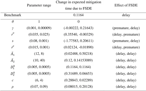
Our model shows how an FSDE can delay or prematurely initiate investments in damage mitigation. This section investigates the sensitivity of this result to the parameter values in the numerical example. Due to the complexity of the model, an analytical comparative analysis is not possible. Instead we report how the change in expected time of mitigation investment in jurisdiction 1 due to the FSDE is impacted by varying each parameter value (Table A1).
Table A1. Sensitivity of model results to a change in parameter values
Parameter range Change in expected mitigation
time due to FSDE Effect of FSDE
Benchmark 0.1164 delay
θ 1 0
γ (0.001, 0.00009) (-0.00222, 0.21643) (premature, delay)
r0 (0.035, 0.025) (0.35540, -0.00329) (delay, premature)
s (0.08, 0.001) (-1.77583, 0.20611) (premature, delay)
rp (0.015, 0.001) (0.02124, -0.01890) (delay, premature)
𝐴̅1 (12, 8) (0.02488, 0.50218) (delay, delay)
𝐴̅2 (10, 40) (0.12, 0.14153089) (delay, delay)
𝐷10 (0.005, 0.0005) (0.1164, 0.1164) (delay, delay) 𝐷20 (0.005, 0.0005) (0.31689, 0.06653) (delay, delay)
c (6, 4) (0.28843, 0.02289) (delay, delay)
35
Derivation of compensated individual timing threshold condition and payment
The payment from agent 2 changes agent 1’s value matching condition to
𝜂𝐷1′ 𝜀0 + 𝐷1′
(𝜌 − 𝛼0)− 𝑍10𝐷1′ 𝜀
0
= 𝐶1+ 𝐷1′
(𝜌 − 𝛼𝑝)− 𝑍1𝑝𝐷1′ 𝜀
𝑝
− 𝛿 [ 1
𝛼0−1 2 𝜎2
ln (𝐷1′ 𝐷0) +
1 𝛼𝑝−1
2 𝜎2 ln (𝐷̅1
𝐷1′) − 𝜏] (𝐴. 13)
and the smooth pasting condition becomes
𝜀0𝜂𝐷 1′ 𝜀
0−1
+ 1
(𝜌 − 𝛼0)− 𝜀0𝑍10𝐷1′ 𝜀
0−1
= 1
(𝜌 − 𝛼𝑝)− 𝜀𝑝𝑍1𝑝𝐷1′ 𝜀
𝑝−1 + 𝛿
𝐷1′[
𝛼0− 𝛼𝑝 (𝛼0−1
2 𝜎2) (𝛼𝑝−12 𝜎2)
] (𝐴. 14)
Combining (A.13) and (A.14) we find 𝜀0
(𝜀0 − 1)𝐶1 = 𝐷1′
𝛼0− 𝛼𝑝
(𝜌 − 𝛼0)(𝜌 − 𝛼𝑝)−
(𝜀𝑝− 𝜀0) (𝜀0− 1) 𝑍1𝑝𝐷1′ 𝜀
𝑝
+ 𝛿
(𝜀0− 1)[
𝜀0
𝛼0−1
2 𝜎2 ln (𝐷1
′
𝐷0) +
𝜀0
𝛼𝑝−1
2 𝜎2 ln (𝐷𝐷̅1
1′) − 𝜀
0𝜏 + 𝛼0− 𝛼𝑝
(𝛼0−1
2 𝜎2) (𝛼𝑝−12 𝜎2)
] (𝐴. 15)
36 𝐷1′ 𝛼0− 𝛼𝑝
(𝜌 − 𝛼0)(𝜌 − 𝛼𝑝) −(𝜀
𝑝− 𝜀0) (𝜀0− 1) 𝑍1𝑝𝐷1′ 𝜀
𝑝 + Λ 𝜀0
(𝜀0− 1) 𝐶1
= 1 (A. 16)
where Λ = (𝜀0𝛿−1)[ 𝜀 0
𝛼0−1 2𝜎2
ln (𝐷1′
𝐷0) +
𝜀0
𝛼𝑝−1 2𝜎2
ln (𝐷̅1
𝐷1′) − 𝜀
0𝜏 + 𝛼0−𝛼𝑝 (𝛼0−1
2𝜎2)(𝛼𝑝− 1 2𝜎2)
].
If 𝐷1′ > 𝐷1∗, agent 1’s payoff from an immediate investment in mitigation under this payment scheme is
𝑊1𝐼 = 𝐶 1+
𝐷1′
(𝜌 − 𝛼𝑝)− 𝑍1𝑝𝐷1′ 𝜀
𝑝
− 𝛿 [ 1
𝛼0−1 2 𝜎2
ln (𝐷1′ 𝐷0) +
1 𝛼𝑝−1
2 𝜎2
ln (𝐷̅1
𝐷1′) − 𝜏] (A. 17)
Comparing (8) and (A.16), δ is found by setting Λ equal to 𝜀 0𝑋−𝐷
1∗Δ
37
Figure 1. Reduction in spread rate of a bioinvasion spreading across N jurisdictions due to control policy implementation at 𝑡𝑖 with i = 1,…, N.
𝐴0
Jurisdiction 1 (𝐴̅1)
Jurisdiction 2 (𝐴̅2)
38
Figure 2. Incentives shaping the private and collective timing of mitigating an uncertain bioinvasion spreading across multiple jurisdictions.
time
time Private cost of delay:
more rapid invasion in jurisdiction 1
Border Damage in jurisdiction 2
Damage in jurisdiction 1
Social cost of delay: expedite invasion in
jurisdiction 2 Do nothing forecast
Do nothing forecast
Border Damage in jurisdiction 2
Damage in jurisdiction 1
Delay to preserve flexibility
Forecast when spread is slowed at cost C
Confidence interval around do nothing forecast Public benefit of delay:
Less likely to invest in control of invasion that was not as damaging as
expected
𝑡̅1
Good news for environment but bad news for return on mitigation investment
39
Figure 3. Effect of FSDE on the timing of mitigation. When the externality elasticity of delay is above (below) ε0 and α0 < ρ (α0 > ρ), agent 1 engages in premature mitigation and must take one for the team to achieve the social optimum mitigation strategy.
ρ α
0
ε0
Premature mitigation Delayed mitigation Premature
mitigation
Delayed mitigation
Delayed mitigation
40
Figure 4. Spread of a bioinvasion along a 1 × 20 km strip managed by two decision makers of equal size. Black lines reflect dollar value damage realized by each agent (𝐷𝑖) as the invasion spreads. The gray line reflects the FSDE (X).
5 10 15 20 A
0.002 0.004 0.006 0.008 0.010 0.012
millions $
𝐴̅1 𝐴̅1+ 𝐴̅2
1 km
𝐴0
41
Figure 5. (a) Discounted expected damage from not investing in mitigation (gray line),
discounted expected damage and mitigation cost from immediately investing in mitigation (black line), and the continuation value 𝑊1𝐶 (dashed line). (b) The FSDE leads to delayed investment in mitigation by agent 1 since 𝐷1∗ falls within a range of damage where the externality elasticity of mitigation delay is below 𝜀0.
0.002 0.004 0.006 0.008 0.010D
0.05 0.10 0.15 millions $
0.002 0.004 0.006 0.008 0.010D
0.5 0.5 1.0 1.5
externality elasticity
𝐷̅1
(b)
𝐷1∗
premature delay
42
Figure 6. Effect of spread uncertainty (s) on the FSDE as the invasion spreads through jurisdiction 1
2 4 6 8 10 A
0.002 0.004 0.006 0.008 0.010 0.012 0.014
X
s = 0.02
s = 0.05