1st – 3rd July 2013 Benchmarking Working Group Workshop Report Executive Summary
National Climatic Data Center (NCDC) of the National Oceanic and Atmospheric Administration (NOAA), Asheville, NC, USA
Attended in person:
Kate Willett (UK), Matt Menne (USA), Claude Williams (USA), Robert Lund (USA), Enric Aguilar (Spain), Colin Gallagher (USA), Zeke Hausfather (USA), Peter Thorne (USA), Jared Rennie (USA)
Attended by phone:
Ian Jolliffe (UK), Lisa Alexander (Australia), Stefan Brönniman (Switzerland), Lucie A. Vincent (Canada), Victor Venema (Germany), Renate Auchmann
(Switzerland), Thordis Thorarinsdottir (Norway), Robert Dunn (UK), David Parker (UK)
A three day workshop was held to bring together some members of the ISTI Benchmarking working group with the aim of making significant progress towards the creation and dissemination of a homogenisation algorithm benchmark system. Specifically, we hoped to have: the method for creating the analog-clean-worlds finalised; the error-model worlds defined and a plan of how to develop these; and the concepts for assessment finalised including a decision on what data/statistics to ask users to return. This was an ambitious plan for three days with numerous issues and big decisions still to be tackled.
The complexity of much of the discussion throughout the three days really highlighted the value of this face-to-face meeting. It was important to take time to ensure that everyone understood and had come to the same conclusion. This was aided by whiteboard illustrations and software exploration, which would not have been possible over a teleconference.
In overview, we made significant progress in terms of developing and converging on concepts and important decisions. We did not complete the work of Team Creation as hoped, but necessary exploration of the existing methods was undertaken revealing significant weaknesses and ideas for new avenues to explore have been found.
The blind and open error-worlds concepts are 95% complete and progress was made on the specifics of the changepoint statistics for each world. Important decisions were also made regarding missing data, length of record and changepoint location
frequency. Seasonal cycles were discussed at length and more research has been actioned. A significant first go was made at designing a build methodology for the error-models with some coding examples worked through and different probability distributions explored.
make their own assessment of the open worlds and past versions of benchmarks. We plan to collaborate with the VALUE downscaling validation project where possible.
From an intense three days all participants and teleconference participants gained a better understanding of what we're trying to achieve and how we are going to get there. This was a highly valuable three days, not least through its effect of focussing our attention prior to the meeting and motivating further collaborative work after the meeting. Two new members have agreed to join the effort and their expertise is a fantastic contribution to the project.
Specifically, Kate and Robert are to work on their respective methods for Team Creation, utilising GCM data and the vector autoregressive method. This will result in a publication describing the methodology. We aim to finalise this work in August.
Follow on teleconferences, Team Corruption will focus on completing the distribution specifications and building the probability model to allocate station changepoints. This work is planned for completion by October 2013. Release of the benchmarks is scheduled for November 2013.
Team Validation will continue to develop the specific assessment tests and work these into a software package that can be easily implemented. This work is hoped to be completed by December 2013, but there is more time available as assessment will take place at least 1 year after benchmark release.
---1st – 3rd July 2013 Benchmarking Working Group Workshop Report National Climatic Data Center (NCDC) of the National Oceanic and Atmospheric
Administration (NOAA), Asheville, NC, USA
Attended in person:
Kate Willett – Met Office Hadley Centre, UK Matt Menne – NCDC, USA
Claude Williams - NCDC, USA
Robert Lund - Department of Mathematical Sciences, Clemson University, USA Enric Aguilar - Centre for Climate Change, Universitat Rovira i Virgili, Spain Colin Gallagher - Department of Mathematical Sciences, Clemson University, USA Zeke Hausfather - Berkeley Earth, USA
Peter Thorne - CICS-NC, USA Jared Rennie - CICS-NC, USA
Attended by phone:
Ian Jolliffe - Exeter Climate Systems, University of Exeter, UK
Lisa Alexander - Climate Change Research Centre, University of New South Wales, Australia
Stefan Brönniman - University of Bern, Switzerland
Lucie A. Vincent - Climate Research Division, Environment Canada, Canada Victor Venema - Meteorologisches Institut, University of Bonn, Germany
Thordis Thorarinsdottir - Statistical Analysis, Pattern Recognition, and Image Analysis (SAMBA), Norwegian Computing Centre, Norway
Robert Dunn - Met Office Hadley Centre, UK David Parker - Met Office Hadley Centre, UK
1) Background:
The Benchmarking project is an important component of the International Surface Temperatures Initiative (ISTI) focussing on building synthetic but realistic analogs to the ISTI databank of surface temperature data from land surface weather stations. Their purpose is to explore a range of known issues for homogenisation algorithms and present a robust means of software testing homogenisation algorithms and other methodological choices made in the process of creating climate data-products.
As described in table 1, this is to be done by first developing a range of synthetic worlds that are free from systematic errors such that they constitute a 'true' climate. Team Creation has been set up to focus on this task.
Plausible error-models, exploring a range of homogenisation issues, will be placed on top of the clean worlds. Team Corruption has been tasked with designing and
implementing these error-models. These error-worlds can then be used alongside the real ISTI databank stations to test the skill of chosen homogenisation algorithms through a range of assessment measures of both climate characteristics and inhomogeneity detection characteristics.
Team Validation is responsible for this part. This assessment will not only allow improved uncertainty quantification of the real-world products but also provide feedback for future improvements of homogenisation algorithms which are essential for ensuring robust long-term climate analysis.
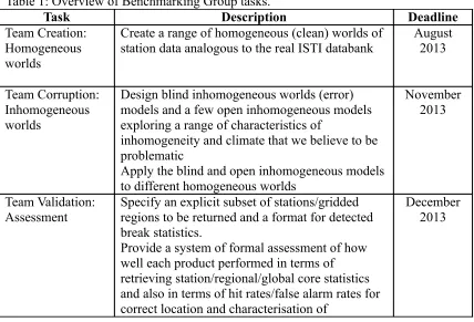
Table 1: Overview of Benchmarking Group tasks.
Task Description Deadline
Team Creation: Homogeneous worlds
Create a range of homogeneous (clean) worlds of station data analogous to the real ISTI databank
August 2013
Team Corruption: Inhomogeneous worlds
Design blind inhomogeneous worlds (error) models and a few open inhomogeneous models exploring a range of characteristics of
inhomogeneity and climate that we believe to be problematic
Apply the blind and open inhomogeneous models to different homogeneous worlds
November 2013
Team Validation: Assessment
Specify an explicit subset of stations/gridded regions to be returned and a format for detected break statistics.
Provide a system of formal assessment of how well each product performed in terms of retrieving station/regional/global core statistics and also in terms of hit rates/false alarm rates for correct location and characterisation of
changepoints.
Provide a concise assessment report for each product.
General: Review
and repeat Review the first benchmark cycle and begin cycle 2... November 2016
The Benchmarking project has been running since September 2010. While a few face-to-face meetings have taken place, these have been largely adhoc at conferences and only a few members at a time. All work has taken place in member's free time (apart from Kate Willett who has 5-10% of time allocated to this) and through
teleconference calls. Hence, progress to date has been slower than first envisaged in addition to the fact that creation of the synthetic yet realistic station data is no trivial task. Getting the station serial correlation and interstation cross-correlations right with globally realistic reconstruction of modes of variability and long-term trends is
complex and although a plausible method (vector autoregression (VAR) over lag 1+) has been investigated there is still a way to go to roll this out globally.
Furthermore, many of the decisions to be made as part of Team Corruption require prior knowledge of global inhomogeneities. Work is ongoing to obtain this
information but in many cases we are limited to making expert judgements of what we think might be the case. Such discussion and information gathering has been time consuming in addition to designing a methodological framework for assigning the various errors to each station.
For Team Validation, while there are many existing methods that will be suitable for assessment both of the climate characteristics and the hit/miss/false alarm rates of the homogenisation algorithms there have been many decisions to make in terms of what spatial and temporal scales are assessed and how to keep everything fair. Other issues include how to estimate the number of correct rejections and how to deal with
submissions using different selections of stations.
It is often difficult to communicate some of the more complex aspects across the telephone, especially when we have members from different backgrounds where common terminology can mean very different things. While progress has been made on all fronts through recent weekly teleconferences, the value of face-to-face time is enormous.
2) Aims:
By the end of this workshop we hoped to have the method for creating the analog-clean-worlds finalised, the error-model worlds defined and a plan of how to develop these and the concepts for assessment finalised including a decision on what
data/statistics to ask users to return. This was an ambitious plan for three days with numerous issues and big decisions still to be made as laid out below for each team:
Big questions for Team Creation
o Is our method going to work over data sparse regions and data dense regions?
o How do we ensure smooth cross-correlations globally across matrix boundaries?
Gibbs sampling?
o How do we compute this efficiently?
R package invoking fortran – speedy but complex and less transparent/ tweakable
R code with parallelisation and bigmatrix – transparent/ tweakable but complex and computer intensive
R code without parallelisation and bigmatrix – transparent/ tweakable but very computer intensive
o Who is going to set up the webpage framework/databank storage framework?
o Who is going to be the handle-turner? Probably Kate?
Big questions for Team Corruption o How blind is blind enough?
o How many different background 'clean worlds'? o How specifically do we build these things?
o How many different things to assess in one world? o Specific decisions to be made:
A - Fix parameters (table from overview_error_worlds.xls) for default world
B - Discuss parameterization (distributions to use)
C - What kind of inhomogeneities do we want to put in the experimental world (#B8)
D - How to implement the seasonal cycle?
E - What should people be asked to homogenise as a minimum (station subset, period etc..
F - How to apply gradual changes?
G - How to package up the error world data?
H - Instructions on how to come and play (will need input from Team Validation too)
Big questions for Team Validation
o How do we assess different style products: grids vs stations? How do we combine information for multiple stations?
o What is our reference homogeneous sub-period (usually the most recent sub-period)?
o What if stations are missed out – should products be penalised and how? - maybe because they are not of interest
- maybe because they are 'too hard' to homogenise o What do we want back from users?
o How do we assess detection/adjustment of gradual inhomogeneities? o Coordinate with VALUE downscaling group in terms of assessment
terminology, tests and software? o Which Levels do we validate:
Level 3 – detailed identification of nature of inhomogeneities (size, duration …)
Level 4 – how realistic/unrealistic, easy/difficult are the various error worlds
3) Daily summaries:
The workshop agenda was deliberately vague to allow free discussion of many of the issues in a non-constrained time frame. Minutes were kept throughout each day using an online forum such that participants at the workshop and members unable to attend could follow and comment at any time. Both the agenda and daily minutes are now available online:
https://sites.google.com/a/surfacetemperatures.org/home/benchmarking-and-assessment-working-group#Minutes. A summary of each day follows below.
Summary of day 1 – July 1st 2013
The focus on this first day was to gain an overview of where we are both in terms of the ISTI plans and current research related to benchmarking of homogenisation algorithms. We began with a welcome and introduction from the director of NCDC, Tom Karl. This was followed by an ISTI overview from Peter Thorne, and ISTI databank overview by Jared Rennie, a Benchmarking working group overview by Kate Willett and then an overview of recent work on creating and using benchmark data to test the pairwise homogenisation algorithm (PHA) performance on the US Historical Climate Network (USHCN) dataset (Williams et al. 2012). This was then followed by a teleconference open to all members and interested parties to discuss Team Creation methods for developing the synthetic analog-clean-worlds. The afternoon was spent going into further details as necessary for Team Creation.
From day one it was concluded that there is high interest in this work but no directly accessible funding streams. Obtaining funding is difficult, especially in the statistical communities as this work is not seen as innovative enough for statistical funding bodies. Climatological funding bodies may favour process based or data-product creation over ISTI's more framework type aims.
In terms of developing the analog-clean-worlds, we established that the VAR method proposed by Robert should be very effective in reproducing the spatio-temporal relationships of the stations. However, there is debate over how to do this based upon inhomogeneous station data that are often short and littered with missing data, which have to be used to build the model in the first place.
There is also debate over how to do this on a global scale. We can attempt to
homogenise the station data first but this will only be as good as available algorithms (which we know are not perfect, hence the purpose of this benchmarking project). Requiring stations to first be homogenised then also limits us to only being able to synthetically reproduce the longer, more temporally-complete stations. Ideally we should synthetically reproduce all stations within the ISTI databank.
non-trivial. Quite how the real global features of ENSO, volcanoes and background climate trends are replicated across all 30,000+ stations is yet to be proven.
One possibility is to use some information from a state of the art (CMIP5) general circulation model (GCM). This is desirable for at least three reasons. Firstly, it ensures some kind of global consistency across the analog-worlds. Secondly, it allows us to create worlds that explore different levels of background trend for example we could use a control run of a GCM that has no persistent long-term trend compared to a high emissions scenario, which contains a large warming trend. Thirdly, a GCM provides 3-dimensional fields for a large collection of atmospheric variables that are physically consistent; radiative and moisture elements can be used to derive more physically realistic error structures for the inserted changepoints for Team Corruption.
It is still not obvious how this blending of a GCM and station properties can be done – methods posed include using a smoothed filter from each GCM gridbox, or the GCM gridbox monthly time series as is, overlaid with higher frequency components of the stations modelled using the VAR method. In both, the real seasonal cycle in the mean and standard deviation can be forced on the analog-stations once the anomaly time series has been created. Alternatively, these features can be built into the statistical model.
These were called the 50/50 method and the 90/10 method respectively due to the percentage of information taken from the GCM verses the station data. However, it is unclear which of these is optimal and there are issues deriving the VAR model for the residual station data after various lower frequency components are removed.
Smoothing the model too much actually removes the ENSO/Volcano features and not smoothing it at all results in modelling only the very high frequency
component/localised climate variability of the station data which is essentially AR(?) time series on top of each station which has have very little cross-correlation with neighbours. This may cause problems when trying to ensure realistic
cross-correlations as these will not be statistically modelled explicitly.
We plan to explore a variety of methods and then test their suitability through realism of station and difference series serial correlations and cross-correlations. We could utilise a likelihood ratio test to quantify which model fits the data best.
We have established that the properties of the station-neighbour/reference are key as many homogenisation groups work on difference series of the station minus a neighbour or neighbour composite. If station and difference series serial correlation and station cross-correlations are similar then we're ok. If not then we are unlikely to be able to perform a fair assessment of such techniques as the posed problem set will be either unrealistically easy or hard.
We should produce stations for as long a time period as we can. If we're using GCMs, most start in 1850 and some go back to 1750. Worlds can be created that are
R or Python are still the software of choice because they are free to use and we wish to encourage both collaborators and others to use our code to explore other
benchmarks once we have published it. In terms of blindness of the analog-worlds, the types of error-worlds being used will be made public but the specifics of which world is which and which station contains what size/shape of changepoints and where will be known only to the 'handle-turner' which will most likely be Kate Willett.
Summary of day 2 – 2nd July 2013:
Day two switched the focus to Team Corruption and design of the error-worlds. We started out with a teleconference with non-attending members. This was led by Victor Venema. We made our way through a list of issues for Team Corruption which
extended beyond the length of the call. Following the call we had a presentation of some work done by Matt Menne, Zeke Hausfather and Victor Venema on creating benchmarks using the USHCN that explored the issue of gradual changepoints in detail. This led on to further discussion of the error-worlds and the key issues laid out in the call that continued throughout the day. We spent some time designing a
probability model with which to allocate changepoints to individual stations given the distributions set out for each world (as in overview_error_worlds.xls).
Blindness:
The basics of what is in the worlds (including the overview_error_world.xls
document?) will be made public but which world is which and the specifics of what and where for each station will not be, nor will the choice of background GCM underlying each analog-clean-world. As the benchmarks are used and assessments returned it will be possible to gain knowledge about which world is which and some of the specifics. Ideally there will be a period over which users can test their
algorithms on the data and then assessment will be done in one go on all entries. However, it was recognized that if this period is too short there are likely to be late entries but if it is too long then users may not see the advantages of coming to play. Users will be allowed to submit multiple entries if they are done simultaneously – e.g., ensemble methods using a range of different parameter choices. Users will not be allowed to submit subsequent entries as they will likely have learned something about what is in the benchmarks from their initial efforts. We should try to speed up the cycles if possible to prevent release of specifics after assessment and optimise the value of the benchmarks to all. However, recycling the benchmarks too frequently may mean that it is difficult to cross-compare products that have been tested against different versions of benchmarks.
Number of clean worlds:
Ideally there will be 3 different GCMs for the blind analog-error-worlds (1:4, 5:10 (not 7), 7) but each world will have its own 'station pink noise' overlaying/merged with the GCM such that every world is unique. Open worlds will use different GCMs and a unique station pink noise overlay for each world.
Fixing parameters:
o We decided that gradual trends are likely to be in more stations (30%) than we first estimated and that they can be shorter/more frequent as
end of gradual trends presumably representing some major change in vegetation or siting characteristics.
o We have decided not to include random errors (i.e., outliers) in the analog-error-worlds as this may contaminate assessment of homogenisation algorithm skill with how skilful the users choice of quality control tests are. We assume that a good QC process has been run on the data and will make this clear when releasing the benchmarks.
o We assume that the distributions of abrupt and gradual changepoint size are Gaussian. We discussed use of Laplace or Pareto flipped back-to-back to provide a peak over the mean changepoint size. However, Gaussian was thought to be sufficient. Although published findings about detected inhomogeneities report fatter tails and a narrow middle with substantial missing allocation around zero (Brohan et al. 2006; Menne et al. 2010; Willett et al. 2013), a study of known changepoints from USHCN metadata shows the distribution to be Gaussian (Menne ???). It is very likely that our current homogenisation algorithms detect the large
changepoints reasonably well (the fat tails – although this may be partially an artefact of detecting one large break where there are multiple small ones of the same direction) but substantially undersample the rest – the middle and much of the sides.
o We assume that the frequency of abrupt changepoints can be modelled using a geometric distribution where each time point is equally likely to contain a changepoint but the number of locations allocated is optimised on a given frequency per century through a given probability parameter. o We assume that only 30% of stations contain gradual changepoints – this
can also be modelled geometrically. Whether an abrupt changepoint co-occurs at the beginning or end can also be modelled given a probability of that occurring. This may result in an extra changepoint being allocated in addition to the average X Per century stipulated. This is not of great concern.
o We assume that the length of a gradual inhomogeneity can be modelled with a discrete distribution such as a Poisson. For this purpose the
distribution cannot be allowed to be 0 or negative but it is likely to be two tailed.
o We have decided not to specify a minimum homogeneous sub-period and allow changepoints to fall where ever, including within the last few years of the record because this is realistic. This will be very hard for algorithms to find but comparisons can be made in anomaly space and between stations with and without changepoints at the end of the record to assess the impact of this.
How to build:
We have established a bottom up station by station probability decision tree with layering.
o Layer one - apply any known/clustered changepoints based on region (nationwide, airport moves)
an appropriate probability distribution. Should one of these changepoints occur simultaneously with a previously assigned changepoint then the latter changpoint will not be applied.
o Layer three – apply either 0 or 1+ gradual changepoints optimising on 30% of stations having at least 1 using a Geometric distribution. There is a small chance of having more than 1 (probability to be decided formally). Decide whether to assign an abrupt changepoint in addition at the
beginning, end, both or neither and assign its size based on a Gaussian distribution. (The graduals could also be assigned within layer 2 rather than necessitating their own layer). Allocate the size of the gradual (and shape – it is likely stepped rather than smooth?) using a Gaussian distribution and duration using a Poisson distribution. Should one of the abrupt changepoints occur simultaneously with a previously assigned abrupt changepoint then the latter changpoint will not be applied.
o Do not locate changepoints within missing data periods - force them to be start or end of missing period.
o Applying some seasonal cycle to a changepoint as opposed to just a mean shift needs more thinking. We estimate that 10-50% of stations have
changes in variance likely joined to temperature, radiation, humidity, wind. CW/LV and the homogenisation list are to provide further advice on this. Gradual changepoints may also have some seasonality or be stepped in nature.
Summary of day 3 – 3rd July 2013:
Day three started with a teleconference to look at some of the issues for Team Validation. This was led by Ian Jolliffe. The group then continued to discuss these issues, but moved back onto the building design for Team Corruption and the specific methods for Team Creation in the afternoon.
Assessment covers four levels:
o Level 1 – correspondence between truth and homogenised series
o Level 2 – whether or not inhomogeneities are found or falsely identified o Level 3 – detailed identification of nature of inhomogeneities (size,
duration …)
o Level 4 – how realistic/unrealistic are the various error worlds
Team Validation will focus on levels 1 and 2 to provide a common assessment of the benchmarks but conduct more detailed assessment including levels 3 and 4 outside of the main assessment framework and encourage others to use the wealth of data provided here to assess performance against the benchmarks which should lead to improved uncertainty estimation and algorithm development.
We need to assess different time periods to account for the changing station density over time and also different user submissions, but should specify a preferred time period to enable useful product-intercomparison.
A webpage hosted or downloadable R package to perform automated assessment would be very useful to provide quick feedback, especially for the open worlds where users may want multiple attempts at the problem. It may be possible to share code (R and web interface code) with the VALUE downscaling intercomparison project which would save us time and perhaps help to develop common terminology and assessment strategies.
As part of assessment of level 1, it is not obvious how to compare variance between the homogenised and clean worlds. This could be assessed as climatological standard deviations for each month or as the standard deviation of the time series or its annual or decadal variance. Ian Jolliffe is to think about ANOVA and other methods.
To assess the impact of station selection we intend to compare level 1 climate measures (e.g., trends) from both the homogenised worlds minus their respective analog-clean-world (subsampled to match homogenised submission) and the
homogenised worlds minus the underpinning GCM model used (complete coverage). Trends can be measured using a percentage trend recovery measure between
homogenised and clean/GCM world then combined across all worlds and methods to give a measure of uncertainty on our current global trend estimates as done in
Williams et al. 2012.
After some further discussion of Team Creation methods we established issues with using stations with some station average removed but queried whether a station minus GCM gridbox would work given the independent time series evolution between the two (GCMs evolve a time series of natural variability (ENSO etc) that is not co-occurrant with reality although we expect long-term trends from historically forced GCMS to be very similar).
This led to discussion of what is a statistical standardised anomaly verses a climate anomaly. Statistical standardised anomalies involve removal of some time-varying mean or linear trend to make them truly stationary prior to calculating the seasonal cycle and subtracting it and the standard deviation and dividing by it – this is not generally what climate scientists consider to be anomalies – climate anomalies often only have a time-stationary seasonal mean removed and are sometimes divided by a time-stationary seasonal standard deviation. This has caused some problems in communication leading to the necessity of an ISTI dictionary to set out all terminology.
4) Overview and major outcomes:
Specific decisions made are noted in the daily summaries. In overview, we made significant progress in terms of developing and converging on concepts and important decisions. We did not complete the work of Team Creation as hoped, but necessary exploration of the existing methods was undertaken revealing significant weaknesses and ideas for new avenues to explore have been found.
The blind and open error-worlds concepts are 95% complete and progress was made on the specifics of the changepoint statistics for each world. Important decisions were also made regarding missing data, length of record and changepoint location
frequency. Seasonal cycles were discussed at length and more research has been actioned. A significant first go was made at designing a build methodology for the error-models with some coding examples worked through and different probability distributions explored.
We converged on what we would like to receive from benchmark users for the
assessment and worked through some examples of aggregating station comparisons of the level 1 climate measures. Contingency tables of some form will be used for level 2 assessment. We also hope to have some online or assessment software available so that users can make their own assessment of the open worlds and past versions of benchmarks.
From an intense three days all participants and teleconference participants gained a better understanding of what we're trying to achieve and how we are going to get there. This was a highly valuable three days, not least through its effect of focussing our attention prior to the meeting and motivating further collaborative work after the meeting. Two new members have agreed to join the effort and their expertise is a fantastic contribution to the project.
5) Plans for here onwards:
A list of actions from the meeting are as follows:
ACTION: Kate to push for research proposals on all aspects of the benchmark project in the UK statistics/climate community
ACTION: Kate is to complete the existing concepts paper draft and circulate ASAP – August at the latest.
ACTION: Claude and Lucie to conclude findings on seasonal cycle in changepoints in the next month – how frequent are seasonally varying changepoints? What are their common characteristics.
ACTION: Victor to contact the homogenisation list about characterising seasonal cycles in changepoints and their frequency.
ACTION: Kate to contact Blair Trewin about size of changepoints (and character) in the tropics. UPDATE: Done
ACTION: Kate to pass R code for Team Creation to Enric to look at and play with – double check it does what we think it does
ACTION: We need standard deviations on the table – overview_error_world.xls to define the distribution.
ACTION: Kate to start an ISTI glossary document in googledocs and invite all ISTI members to contribute. UPDATE: Done
ACTION: Ian to think about use of ANOVA or other methods for comparing the variance between two time series.
ACTION: Discuss how best to deal with hits/misses/false alarm rates in future conference call.
ACTION: Victor to put some numbers on how big a window we should allow surrounding changepoint location – suggestion that the window should be larger for smaller changepoints as these are harder to locate accurately. UPDATE: Victor is no longer sure whether such an equation makes sense as it depends on the SNR and thus on the reference, which may be computed in many ways. Maybe first discuss this in Team Validation.
ACTION: Claude to look at PHA results to try and characterise some of the gradual changepoints in particular the frequency of the slopes, their size, their duration and if anything can be said about their character – are they linear or stepped or other?
Specifically, Kate and Robert are to work on their respective methods utilising GCM data and the VAR(?) method. This will result in a publication describing the
methodology. We aim to finalise this work in August.
Follow on teleconferences will focus on completing the distribution specifications within the overview_error_world.xls document and the building the probability model to allocate station changepoints. This work is planned for completion by October 2013. Release of the benchmarks is scheduled for November 2013.
Team Validation will continue to develop the specific assessment tests and work these into a software package that can be easily implemented. This work is hoped to be completed by December 2013, but there is more time available as assessment will take place at least 1 year after benchmark release.
6) Acknowledgements:
Thanks to Matt Menne for sponsoring the entire workshop through his PECASE funding which covered NCDC hosting costs, travel costs for Enric Aguilar and Kate Willett and subsistence costs for all non-local participants. Thanks also to Matt for coordinating and hosting the workshop in addition to keeping us topped up with espressos. Thanks to Robin Evans for sorting out all of the logistics and looking after us all so well during our workshop including keeping us well fuelled with sugar and caffeine. Thanks to Tom Karl for giving us such a good welcome on our first morning and allowing us all to use the NCDC facilities. Thanks to Tom Peterson for saving Kate Willett from almost certain jetlag by taking her to an aerial skills class in the evening. Thanks to all participants (who attended in person and over the phone) for all of their continued contributions and enthusiasm throughout the workshop and over the course of the project so far. All efforts have come largely from people's free time.