Technical Appendix for the R Package SAMURAI
Last updated: April 2014.
1 Formatting a data set file for use by SAMURAI
1.1 Binary outcomes
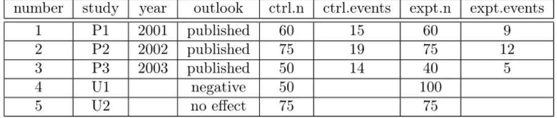
The data set should have the same column headings as those in the example below in Table 1. Table 1: An example of a data set with studies with binary outcomes.
number study year outlook ctrl.n ctrl.events expt.n expt.events
1 P1 2001 published 60 15 60 9
2 P2 2002 published 75 19 75 12
3 P3 2003 published 50 14 40 5
4 U1 negative 50 100
5 U2 no effect 75 75
The outlook of a study can be one of the following: “published”, “very positive”, “positive”, “no effect”, “negative”, “very negative”, “very positive CL”, “positive CL”, “current effect”, “negative CL”, or “very negative CL”.
ctrl.n and expt.n refer to the sample sizes of the control and experimental arms, respectively. ctrl.events and expt.events refer to the numbers of events within the control and experimental arms, respectively.
1.2 Continuous outcomes
A data set with continuous outcomes can be in one of two formats. 1.2.1 Means and standard deviations
For studies containing the mean effect and its standard deviation for each arm of a published study, the column headings should be the same as in the example below in Table 2.
Table 2: An example of a data set with means and standard deviations for each treatment arm. number study year outlook ctrl.n ctrl.mean ctrl.sd expt.n expt.mean expt.sd
1 P1 2001 published 40 92 20 40 94 12.9
2 P2 2002 published 50 88 26 50 82.20 11.3
3 P3 2003 published 60 82 22 60 0.90 25.1
4 U1 negative 50 50
5 U2 no effect 75 75
ctrl.n and expt.n refer to the sample sizes of the control and experimental arms, respectively. ctrl.mean and expt.mean refer to the mean effect size within the control and experimental arms, respectively.
ctrl.sd and expt.sd refer to the standard deviation of the effect size within the control and experimental arms, respectively.
1.2.2 Standardized mean differences (SMD)
For studies containing data on the standardized mean difference (SMD) and its variance for each published study, the column headings should be the same as in the example below in Table 3. The SMD should be equivalent to Hedges’ g.
Table 3: An example of a table with standardized mean differences (SMD).
number study year outlook ctrl.n expt.n smd smd.v
1 P1 2001 published 60 60 0.095 0.033
2 P2 2002 published 65 65 0.277 0.031
3 P3 2003 published 40 40 0.367 0.05
4 U1 negative 100 100
5 U2 no effect 75 75
ctrl.n and expt.n refer to the sample sizes of the control and experimental arms, respectively. smd is the SMD and smd.v is its variance.
2 Importing a data set file
The R function read.csv() can be used to import CSV files that separate values by commas. The R function read.csv2() can be used to import CSV files that separate values by semi-colons (as is done on computers with Microsoft Windows with German language settings).
3 Pseudocode of forestsens()
Step 0: (Optional) Designate all unpublished studies to have the same outlook (i.e. the same risk ratio). The user can override the outlooks of the unpublished studies with a specified outlook by using the option outlook. For example, to assign the outlook “no effect” to all unpublished studies, we can specify the option outlook=“no effect”.
3.1 For studies with binary outcomes
Step B1: Subset the published studies. Calculate the log risk ratio and its variance for each of the published studies. Calculate a summary effects across the collectoin of published studies using a random effects model. Let k denote the number of published studies included in the meta-analysis. For the j-th published study, with j 2 {1, . . . , k}, denote x0j events out
of n0j persons in the control group, and x1j events out of n1j persons in the treatment group.
Table 4: Published studies
Intervention Control
Study Events Sample size Events Sample size
Published study 1 x11 n11 x01 n01
... ... ... ... ...
Published study k x1k n1k x0k n0k
Totals over published studies A =Pk
Step B2: For each individual published study Let ˆp0j = x0j/n0j be the estimate of the rate of
events in the control group, and ˆp1j = x1j/n1j be the estimate of the rate of events in the treatment
group. Calculate the estimate of the log risk ratio as log dRRj= log (ˆp1j/ˆp0j) = log
✓x
1j/n1j
x0j/n0j
◆ and its approximate variance as
d var⇣log dRRj ⌘ = 1 x0j + 1 x1j 1 n0j 1 n1j .
The lower and upper bounds of the (1 ↵) confidence interval (with ↵ 2 [0, 1]) of the risk ratio are then defined to be LCLj,1 ↵= exp ( log dRRj z1 ↵/2 r d var⇣log dRRj ⌘) , U CLj,1 ↵= exp ( log dRRj+ z1 ↵/2 r d var⇣log dRRj ⌘) ,
where z1 ↵/2is selected such that for a standard normal random variable Z, P (|Z| > z1 ↵/2) = 1 ↵.
The default confidence level is 95%.
Step B3: For the published studies collectively To get a summary effect of the published studies using a random effects model, the binary outcome data are converted to log risk ratios. (See Step B2.) Then a summary effect is calculated using a random effects model via the DerSimonian & Laird method [DS86; BHHR09]. This is accomplished using the R package metafor function rma() with the option method=DL. The default confidence level is 95%.
DerSimonian & Laird method The steps of the DerSimonian & Laird method are as follows: 1. For each study, calculate the estimate of the variance ˆvj =vard
⇣ log dRRj
⌘
. (See Step B2.) 2. Estimate the between-studies variance ⌧2 as follows: Weight each study by the inverse of the
variance. wj = 1/ˆvj. Add up the weights. W = Pkj=1wj. Also calculate the following quantities:
W 2 =Pkj=1w2
j; W Y =
Pk
j=1wjyj, W Y 2 =Pj=1k wjy2j , where yjis the standardized mean difference
in the j-th study. Then an estimator of ⌧2 is:
ˆ ⌧2= W Y 2 (W Y )2 W (k 1) W W 2 W .
3. For each study, define the total variance as vj+ ⌧2. Weight each study by the inverse of the
estimated total variance. w⇤
j = 1/(ˆvj+ ˆ⌧2). (Note that the between-studies variance and the
within-studies variances are assumed to be independent of each other.) Add up these weights. W⇤=Pk j=1w⇤j.
Also calculate W⇤Y =Pk
j=1wj⇤yj. Then a random-effects model effect for the summary log risk ratio
is M⇤= W⇤Y /W⇤, and its approximate variance is V
M⇤ = 1/W⇤.
Then the estimate of the summary log risk ratio is
log dRRpub= W⇤Y /W⇤,
The lower and upper bounds of the (1 ↵) confidence interval (with ↵ 2 [0, 1]) of the summary risk ratio are then defined to be
LCLpub,1 ↵= exp
(
log dRRpub z1 ↵/2
r d
var⇣log dRRpub
⌘) , U CLpub,1 ↵= exp ( log dRRpub+ z1 ↵/2 r d
var⇣log dRRpub
⌘) ,
where z1 ↵/2is selected such that for a standard normal random variable Z, P (|Z| > z1 ↵/2) = 1 ↵.
Detailed examples can be found in Chapter 14 of Borenstein, Hedges, Higgins, & Rothstein [BHHR09]. Those examples involve log odds ratios but the procedure is the same for log risk ra-tios.
Step B4: For the unpublished studies, impute the number of events in the control arms, based on the risk of events in the control arms of the published studies. No random vari-ation is used to impute these numbers. We assume that the rates of events in the control arms are the same across all published and unpublished studies. Let m denote the number of unpublished studies included in the meta-analysis, and let ˆp0,pub= C/n0denote the estimated proportion of events
across the control arms of all published studies. For the i-th unpublished study (i 2 {1, . . . , m}), with n0i persons in the control arm (and n1i persons in the treatment arm), impute the number of events
within the control arm to be
x0i= [n0ipˆ0,pub],
that is, n0ipˆ0,pubrounded to the nearest integer. Repeat for all m unpublished studies.
Step B5: Assign risk ratios to all defined outlooks. Defined outlooks include outlooks based on the confidence interval of the log risk ratio of the published studies. The default risk ratios assigned to each of the outlooks are as follows, depending on whether the event is desirable or not.
Table 5: Default risk ratios assigned to unpublished studies
Outlook higher.is.better=TRUE higher.is.better=FALSE
very positive 3 0.33
positive 2 0.5
no effect 1
negative 0.5 2
very negative 0.33 3
very positive CL U CLpub,0.95 LCLpub,0.95
positive CL 0.5(dRRpub+ U CLpub,0.95) 0.5(dRRpub+ LCLpub,0.95)
current effect RRdpub
negative CL 0.5(dRRpub+ LCLpub,0.95) 0.5(dRRpub+ U CLpub,0.95)
very negative CL LCLpub,0.95 U CLpub,0.95
Note that outlooks denoted with “CL” are defined according to a confidence interval of the risk ratio of the published studies collectively. (See Step B3.)
Step B6: For each of the unpublished studies, estimate the proportion of events in the intervention arm, based on the risk ratio assigned to the study outlook. Then impute the number of events in the intervention arm randomly from a binomial distribution. Let mt m be the number of unpublished studies in the meta-analysis with outlook t, and denote
the proportion of events in the treatment and control arms of such studies as p1t and p0t respectively.
Note thatPtmt= m. Extract the assigned risk ratio RRt= p1t/p0t for studies with outlook t from
Table 5. Estimate the proportion of events in the treatment arms by rearranging the formula for risk ratio:
ˆ
p1t= RRt· bp0t = RRt· bp0,pub.
(Note that ˆp0t =pb0,pub since we have assumed that the true rate of event in the control arm is the
same across all studies.)
For the i-th unpublished study, having outlook t and treatment sample size n1i, impute the number
of events within the treatment arm to be x1i = [X],where X is a random variable from a binomial
distribution with mean yi= n1ipˆ1t and variance vi= ˆp1t(1 pˆ1t)/n1i).
Step B7: For each unpublished study, calculate the standard error of the log risk ratio using the imputed figures for the numbers of events in the control and intervention arms. Calculate a summary effect across the collection of unpublished studies using a random effects model. Calculate a summary effect across all (published and unpublished) studies in the meta-analysis using a random effects model. These summary effects are calculated using the DerSimonian & Laird method, as detailed under Step B3.
Step B8: Graph a forest plot of individual and aggregate results. This is done using the metafor functions forest() and addpoly() [WV10].
Step B9: (Optional) Repeat Steps B1 to B8 for each outlook. The user can generate one plot for each of the ten outlooks defined for unpublished studies (see Table 5) by using the option all.outlooks=TRUE.
3.2 For studies with continuous outcomes
Step C1: If the data is in the form of means and standard deviations, convert the data in each study to a standardized mean difference (Hedges’ g). The following procedure is from [BHHR09].
The following formula for pooled within-groups standard deviation is used: swithin=
s
(nctrl 1)s2ctrl+ (nexpt 1)s2expt
nctrl+ nexpt 2
This is used to estimate Cohen’s d:
d =xexpt xctrl swithin
Cohen’s d can be converted into Hedges’ g using the conversion factor
J = 1 3
4(nctrl+ nexpt 2) 1
. Hedges’ g is then
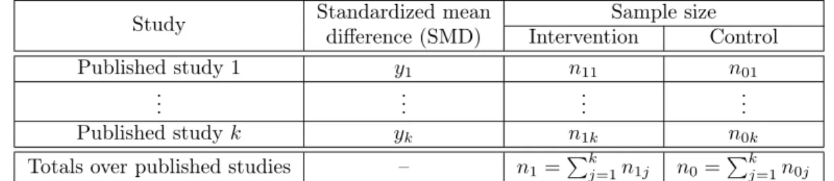
Step C2: Subset the published studies. Impute the variance of the SMD of each study using a ‘very good’ approximator mentioned by Borenstein [CHV09, 226]. Calculate the summary SMD for the published studies with a random-effects model using the method by DerSimonian & Laird [DS86]. Let k denote the number of published studies included in the meta-analysis, indexed by j 2 {1, . . . , k}.
Table 6: Published studies
Study Standardized meandifference (SMD) InterventionSample sizeControl
Published study 1 y1 n11 n01
... ... ... ...
Published study k yk n1k n0k
Totals over published studies – n1=Pkj=1n1j n0=Pkj=1n0j
Step C3: For each published study Imputing the variance of the SMD can be done as follows if we assume the SMD is equivalent to Hedges’ g: Let ⌫ = k 1 and J⌫= 1 3/(4⌫ 1). J⌫ is known as
a correction factor for converting Cohen’s d to Hedges’ g. Assuming the SMD is equivalent to Hedges’ g, convert the SMD to Cohen’s d using the formula d = g/J⌫. Then use a ‘very good’ approximator
of the variance vd of Cohen’s d mentioned by Borenstein [CHV09, 226]:
ˆ vd= n1+ n0 n1n0 + d2 2(n1+ n2),
where n0, n1 are as defined in Table 6.
The variance vg of Hedges’ g is then approximated by the following:
ˆ
vg= J⌫2vˆd.
Then define the lower and upper bounds of the (1 ↵) confidence interval (with ↵ 2 [0, 1]) of the SMD as LCLi,1 ↵= exp n yj z1 ↵/2 p bvg o , U CLi,1 ↵= exp n yj+ z1 ↵/2 p bvg o ,
where yj denotes the SMD of the j-th study, and z1 ↵/2 is selected such that, for a standard normal
random variable Z, P (|Z| > z1 ↵/2) = 1 ↵.
Step C4: For the published studies collectively To get a summary effect of the published studies using a random effects model, use the DerSimonian-Laird method [DS86; BHHR09] to calculate ypub,
the standardized mean difference (SMD) across all published studies. This is accomplished using the R package metafor function rma() with the option method=DL. The default confidence level is 95%. DerSimonian & Laird method The steps of the DerSimonian & Laird method are as the same as under Step B3, except as follows:
1. For each study, calculate the estimate of the variance of the SMD: ˆvj=var (yd j), where yj is the
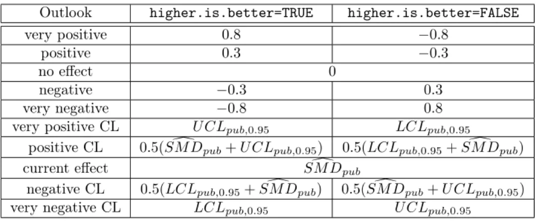
Step C5: Assign SMD to all defined outlooks. Defined outlooks include outlooks based on the confidence interval of the SMD of the published studies collectively. The default risk ratios assigned to each of the outlooks are as follows, depending on whether the event is desirable or not.
Table 7: Default SMD assigned to unpublished studies
Outlook higher.is.better=TRUE higher.is.better=FALSE
very positive 0.8 0.8
positive 0.3 0.3
no effect 0
negative 0.3 0.3
very negative 0.8 0.8
very positive CL U CLpub,0.95 LCLpub,0.95
positive CL 0.5( dSM Dpub+ U CLpub,0.95) 0.5(LCLpub,0.95+ dSM Dpub)
current effect SM Dd pub
negative CL 0.5(LCLpub,0.95+ dSM Dpub) 0.5( dSM Dpub+ U CLpub,0.95)
very negative CL LCLpub,0.95 U CLpub,0.95
Note that outlooks denoted with “CL” are defined according to a confidence interval of the risk ratio of the published studies collectively. (See Step C4.)
Step C6: For each unpublished study, impute the SMD and its variance. Based on the outlook of the unpublished study, impute the SMD using Table 7. Then employ Borenstein’s ‘very good’ approximator of vd(as we did in Step C3).
Step 7: Calculate a summary effect across the collection of unpublished studies using a random effects model. Calculate a summary effect across all (published and unpublished) studies in the meta-analysis using a random effects model. These summary effects are calculated using the DerSimonian & Laird method, as detailed under Step C4.
Step 8: Graph a forest plot of individual and aggregate results. This is done using the metafor functions forest() and addpoly() [WV10].
Step 9: (Optional) Repeat Steps C1 to C8 for each outlook. The user can generate one plot for each of the ten outlooks defined for unpublished studies (see Table 7) by using the option all.outlooks=TRUE.
References
1. [BHHR09] Borenstein, Hedges, Higgins, & Rothstein. Introduction to Meta-analysis. UK: Wiley, 2009.
2. [CHV09] Cooper, Hedges, & Valentine, eds. Handbook of Research Synthesis & Meta-analysis, 2nd ed. NY: Russell Sage Foundation, 2009.
3. [DL86] Rebecca DerSimonian and Nan Laird. “Meta-analysis in clinical trials.” Controlled Clin-ical Trials 7:177-188 (1986).
4. [WV10] Wolfgang Viechtbauer (2010). “Conducting Meta-Analyses in R with the metafor Pack-age.” Journal of Statistical Software, 36:3 (August 2010).