T E C H N I C A L A D V A N C E
Open Access
Crude incidence in two-phase designs in
the presence of competing risks
Paola Rebora
1*, Laura Antolini
1, David V. Glidden
2and Maria Grazia Valsecchi
1Abstract
Background: In many studies, some information might not be available for the whole cohort, some covariates, or even the outcome, might be ascertained in selected subsamples. These studies are part of a broad category termed two-phase studies. Common examples include the nested case-control and the case-cohort designs. For two-phase studies, appropriate weighted survival estimates have been derived; however, no estimator of cumulative incidence accounting for competing events has been proposed. This is relevant in the presence of multiple types of events, where estimation of event type specific quantities are needed for evaluating outcome.
Methods: We develop a non parametric estimator of the cumulative incidence function of events accounting for possible competing events. It handles a general sampling design by weights derived from the sampling probabilities. The variance is derived from the influence function of the subdistribution hazard.
Results: The proposed method shows good performance in simulations. It is applied to estimate the crude incidence of relapse in childhood acute lymphoblastic leukemia in groups defined by a genotype not available for everyone in a cohort of nearly 2000 patients, where death due to toxicity acted as a competing event. In a second example the aim was to estimate engagement in care of a cohort of HIV patients in resource limited setting, where for some patients the outcome itself was missing due to lost to follow-up. A sampling based approach was used to identify outcome in a subsample of lost patients and to obtain a valid estimate of connection to care.
Conclusions: A valid estimator for cumulative incidence of events accounting for competing risks under a general sampling design from an infinite target population is derived.
Keywords: Two-phase design, Competing risks, Crude incidence, Case-control, Case-cohort, Missing data, Subdistribution hazard
Background
In many longitudinal studies, some information might not be measured/available for the whole cohort, in fact biomarkers/additional covariates, or even outcome, might be ascertained only in selected subsamples. These stud-ies are part of a broad category termed two-phase studstud-ies [1], in fact they imply two sampling phases: the first one being usually a random sample from the target popu-lation, ending up in the entire cohort (phase I sample), and the second one applying some kind of sampling (e.g. efficient or of convenience) to collect additional infor-mation or the selection of subjects with no missing data
*Correspondence: [email protected]
1Center of Biostatistics for Clinical Epidemiology, School of Medicine and Surgery, University of Milano-Bicocca, via Cadore 48, 20900 Monza, Italy Full list of author information is available at the end of the article
(phase II sample). Common examples of efficient second phase sampling include the nested case-control and the case-cohort designs [2–5]. In other situations the outcome itself is collected only for a subsample [6]. Two-phase sam-pling, or more generally, multiphase samsam-pling, is a general design that includes any valid probability sample of the data, in which each subsampling can depend on all the currently observed data at each step [7]. The actual sam-pling probabilities will depend on the specific design. The acknowledgement of these sampling phases, even in the commonly applied designs, can be very useful to improve efficiency and to allow flexibility in the analysis (e.g. dif-ferent time-scales or difdif-ferent models can be applied) by using information available for the whole cohort [8].
Efficient designs are particularly useful to identify new biomarkers when the combination between large cohorts
and expensive new technologies make it infeasible to mea-sure the biomarkers on the entire cohort. The Women’s Health Initiative program, for example, stored serum and plasma from participants and used them for specialized studies [9]. Also the Cardiovascular Health Study col-lected DNA from most participants to study different genetic factors underlying cardiovascular or other dis-eases and only subsets of the cohort have been genotyped in different projects [10].
In our first motivating clinical example, the aim was to evaluate the role of different genetic polymorphisms on treatment failure due to relapse in childhood acute lymphoblastic leukemia (ALL) using clinical information and biological samples available from a clinical trial that enrolled nearly 2000 patients. In this situation, a parsi-monious use of these specimens motivated the choice of an efficient/optimal two-phase sampling design [11]. We present also a further application where the aim was to estimate engagement to care of HIV patients in resource limited settings. Here the outcome itself was missing in a group of patients due to possibly informative loss to follow-up. The outcome was tracked in a random sam-ple of those lost to follow-up to obtain a valid estimate of engagement to care [12].
For two-phase studies, appropriate weighted survival estimates have been derived, both in the presence of addi-tional covariates measured in the second phase [7, 13, 14], as well as in cohorts where the outcome/follow-up is not available for everyone [15]. A Cox model adapted for two-phase designs has also been derived [14]. However no estimator of cumulative incidence accounting for compet-ing events in the general framework of two-phase designs has been proposed, while it has been developed for spe-cific designs, such as nested case-control studies [16, 17]. This is relevant in the presence of multiple types of events, such as relapse and (toxic) death in cancer patients, as in the motivating examples presented here, where estimation of event type specific quantities are needed for evaluating outcome.
The aim of this paper is to develop a non parametric estimator of the crude incidence of events accounting for possible competing events in the general framework of two-phase designs, where subgroups of analysis might be defined according to explanatory variables ascertained in the phase II sample, or the outcome itself assessed only in the second phase sample.
In the Methods section we propose a weighted crude incidence estimator for application in two-phase designs. The theoretical properties of the proposed method are derived in appendix and investigated through simulations under different scenarios, which results are reported in Results section. In this section we also report the exam-ples on childhood ALL and HIV patients. Conclusions is dedicated to the discussion.
Methods
Notation and basics
LetT be the failure time variable and suppose there are
Kpossible causes of failure denoted byε=1, 2,. . .K. Let the cause-specific hazard function of thekthevent be:
λk(t)= lim dt→0
1
dtP(t≤T<t+dt;ε=k|T≥t)
andk(t)= t
0λk(s)ds. Define
Fk(t)=P(T ≤t;ε=k) (1)
as the probability that a failure due to causek occurs by timet, that is the quantity that we aim to estimate. Define alsoS(t)=P(T >t)=1−kFk(t)as the probability of surviving from any cause of failure.
A convenient representation of the crude incidence function (1) as product limit estimator naturally arises starting from the subdistribution hazard introduced by Gray [18] and defined as:
λ∗k(t)=dtlim→0 1
dtP{t≤T <t+dt;ε =k|T ≥t∪(T <t;ε=k)}
(2)
This hazard has been shown to be very useful to com-pare the crude cumulative hazard functions in differ-ent groups, since it restores a one-to-one relationship between the hazard and the cumulative probability of a particular failure type:Fk(t) = 1−exp
−∗
k(t)
= 1−
s≤t
1−∗k(ds), with ∗k(t) = 0tλ∗k(s)ds and where the product integral notationis used to suggest a limit
of finite products [18, 19]. Of note, the one-to-one
relationship between the hazard and the cumulative prob-ability is not satisfied from the cause-specific hazard in the presence of competing events [20]. The subdistribu-tion hazard can be thought as the hazard of an artificial variableTk∗ = T ·I{ε=k} + ∞ ·I{ε=k}that extends to infinity the time to event kwhen another competing event is observed. In fact, for any finitet,Tk∗≤tis equiv-alent to T ≤ t and ε = k; thus, given definition (1),
P Tk∗≤t=Fk(t). The definition ofTk∗is consistent with the argument that when an event other thankoccurs as first, the latter will never be observed as first and thus the corresponding time is infinity.
Let(Ti,εi,Ci,Zi), withi = 1. . .N, beN independent replicates of (T,ε,C,Z), where C is the censoring time andZa vector of covariates. We will refer to theseN sub-jects as the phase I sample. Define X = min(T,C)and
= I(T ≤ C). We will assume that failure and censor-ing times are conditionally independent, T ⊥ C|Z. Let
Suppose that complete information on(Xi,iεi,Zi) is available only for a subsetn<Nof subjects drawn based on a possibly complex sampling design and let ξi indi-cate whether subject i is selected into this sample. We will refer to then = iξi subjects as the phase II sam-ple, even if multiple phases of sampling could actually be involved to obtain the final complete sample [7]. Let
πi=P(ξi=1|Xi,iεi,Zi)being the inclusion probability of subjectifor the phase II sample, conditional on being selected at the first phase. In a random sample this proba-bility is equal for every subject. However sampling is often stratified on some variables to increase efficiency; in this case, the probability to be selected for the phase II sample is common for all subjects in the same stratum and differs between strata. In particular, it is usually higher for the more informative strata (e.g. strata including subjects with the event of interest as in case-control studies). For nested case-control designs the sampling probability of cases will be 1, while the one of controls might be derived as the probability that individualiis ever selected as control, fol-lowing Samuelsen [4]. We denote the pairwise sampling probability for any two subjects (i,j, withi = j) byπij = P(ξi = 1,ξj = 1|Xi,iεi,Zi,Xj,jεj,Zj). As commonly assumed in survey theory, the sampling method should have the following properties: the sampling probabilities
πiandπijmust be non zero for alli,jin the population and must be known for eachi,jin the sample [7].
Incidence estimation in the presence of competing risks
Overall survival/incidence estimate
Under a two-phase design it is common to be interested in estimating survival in subgroups related to variables ascer-tained only in phase II sample (i.e. biomarkers). Another possible situation is that, instead of covariates, the out-come itself is not available for the whole cohort. Thus, in both cases an estimate of the incidence of event using only the phase II sample is very useful. The total num-ber of events of typek up tot and the total number of persons at risk at time t for the entire phase I sample can be estimated from the phase II sample (accounting for the sample design) byNˆ·k(t) =
N
i=1[ξiNik(t)/πi] and ˆ
Y·(t) = Ni=1[ξiYi(t)/πi], respectively. Note that these estimates are valid under general sampling designs, where
πiandπij, the so-called ‘design weights’, are known for the observations actually sampled [21].
The estimate of the overall survival has been shown by several authors in different contexts of complex sampling [13–15]:
ˆ S(t)=
s≤t
1− ˆ(ds) (3)
where the overall hazard can be obtained by (t)ˆ =
K
k=1ˆk(t) and ˆk(t) = t
0Nˆ·k(ds)/Yˆ·(s) [22]. It has
been shown that√N[(ˆ t)−(t)] converges weakly to a zero-mean Gaussian process [14, 15].
Competing risk
The goal is to estimate the crude incidence of a given cause
k,Fk(t)=1−s≤t
1−∗k(ds), using the phase II sam-ple, which is also called subdistribution function and is the probability that a failure due to causekoccurs within
t[23, 24]. The estimate of∗k(t)is based on the count of events due to causekand the count of subjects at risk for
Tk∗, denoted byYˆ·∗k(s)(see Appendix A.1):
ˆ Y·∗k(s)=
N
i=1 ξi πi
Yi(s)+ N
i=1 ξi πi
⎡
⎣
l=k
Nil(s−)· ˆG(s−|Xi−) ⎤ ⎦
(4)
The estimate of the cumulative subdistribution haz-ard in (2) can now be estimated, using only the phase II sample, by:
ˆ ∗k(t)=
t0 ˆ N·k(ds)
ˆ
Y·∗k(s) . (5)
Note the complement ofFk(t)can be thought as the sur-vival probability ofTk∗ [18, 20, 25], thus a product limit type estimator can be directly derived as:
ˆ
Fk(t)=1− s≤t
1− ˆ∗k(ds)=1− s≤t
1−Nˆ·k(ds) ˆ Y·∗k(s)
(6)
Interestingly, this estimator is algebraically equivalent to the Aalen-Johansen type estimator, shown by [18] for random sampling, and in the Appendix A.2 for general sampling:
ˆ
Fk(t)=1− s≤t
1− ˆ∗k(ds)= t
0 ˆ
S(s−)ˆk(ds) (7)
It is easy to see that in the absence of competing events, ˆ
Y·∗k(s) in (4) degenerates to the usual risk setYˆ·(s), thus ˆ
∗k(t)= ˆ(t)andFˆk(t)equals the complement of 1 of the weighted Kaplan-Meier estimator for two-phase studies [13]. Under no censoring, the weight G(sˆ −|Xi) becomes 1 and the risk set Y·∗k is eroded in time only by events of type k, therefore Fˆk(t) degenerates into the propor-tion of events of typekestimated by the phase II sample (weighted number of events of typekout of the estimated total size of the cohort, phase I). If every subject in phase I is sampled (ξi = 1∀i), then (5) becomes the standard subdistribution cumulative hazard [19, 20] and (6) the standard estimator of the crude incidence.
also be applied on subgroups defined by Z. The censor-ing probabilityG(t)should also be estimated in subgroups defined by Z. The overall estimator is reasonable when we make the more restrictive assumptionT ⊥ C, other-wise separate estimators conditional onZwould be more appropriate (and eventually an average, weighted on the frequencies of Z, between the conditional estimates).
Variance and confidence intervals
Following Breslow and Wellner [26], we can express √
Nˆ∗k(t)−∗k(t) = √N˜∗k(t)−∗k(t) + √
Nˆ∗k(t)− ˜∗k(t) where ˜∗k(t) represents the crude cumulative incidence estimator that we would have obtained if complete information(Xi,iεi,Zi)was known for all the subjects in phase I sample (i = 1. . .N) [18]. The two terms are asymptotically independent [14, 26]. The first term converges weakly to a zero-mean Gaussian process [19] with covariance that we denote as σkI2(t). By the arguments in Appendix A.3, the second term converges weakly to a zero-mean Gaussian process with covarianceσkII2 (t). Hence,√N
ˆ ∗
k(t)−∗k(t)
converges weakly to a zero-mean Gaussian process with covariance being the sum of the contribution of each sampling phase:
σ2
k(t) = σkI2(t) + σkII2 (t). The first one represents the irreducible minimum uncertainty that would remain if everyone in phase I would be sampled and the second one accounts for the fact that complete information is available only in the phase II sample [13, 14, 26].
Each contribution to the variance can be estimated by the influence function approach [27]. The influence func-tion of an estimator describes how the estimator changes when single observations are added or removed from the data and has the property that the difference between the estimate and the population quantity can be expressed as the sum of influence functions over all the subjects in the sample. By denoting withzik∗(t)the influence function of subjectionˆ∗k(t)we have that [28]:
ˆ
∗k(t)−∗k(t)= N
i=1
zik∗(t)+o(1/√N) (8)
The influence function of subjectionˆ∗k(t) has been derived in Appendix A.4.
By using the Horvitz-Thomposon variance [29] on the weighted influence function, the contribution of the vari-ance of phase II will be:
ˆ σ2
kII(t)= ˆvar N
i=1 ξi πi
z∗ik(t)
=
= n
i=1 n
j=1
z∗ik(t)·z∗jk(t) πi·πj −
z∗ik(t)·z∗jk(t) πij
(9)
For phase I, the variance σˆkI2(t) can also be estimated using (9) by setting sampling probabilities to 1 [13].
Given the one-to-one relationship between Fk(t) and ∗
k(t), the variance of the crude cumulative incidence (6) can now be estimated as:
ˆ varFˆk(t)
=1− ˆFk(t) 2
· ˆσ2
k(t) (10)
In analogy with the survival estimate for two-phase designs, we derived confidence intervals for (6) on the logarithm scale by:
exp
log[Fˆk(t)]±qα/2
1− ˆFk(t) ˆ Fk(t)
ˆ σk(t)
(11)
whereqα/2denotes theα/2 quantile of the standard
Gaus-sian distribution.
Software
By using suitable weights for both study design and cen-soring, any software allowing for time dependent weights can be used to derive the modified risk set and to estimate the crude cumulative incidence function (6). These weights have been implemented in R in function crprepin themstatepackage [30] and in STATA in the stcrprepfunction. However, any software can be used to derive the ingredients for the modified risk set in (4) and these can be used to estimate (6) and its variance by the Horvitz-Thompson approach.
The complete code to compute this estimate has been
developed in R software [31] using thesurveypackage
[32] and is available at [33]. An example of the applica-tion of this funcapplica-tion is given in the subsecapplica-tion Genotype ascertained on a subset of a clinical trial cohort.
Results
Simulations
Simulations protocol
We considered two competing events with independent latent times T1andT2 and constant marginal hazard of
0.1, the crude incidences are thenF1(t) =F2(t) = 12(1−
e−0.1t). We focused on the crude incidence of event 1 up tot = 2 units of time (i.e. years). This implies a fraction of 82 % with no events att = 2 (administrative censor-ing) and a crude incidence of about 9 %. The independence between the latent timesT1andT2is not restrictive given
the non identifiability issue [34]. The censoring time fol-lowed an uniform distribution on ranges (0.5,30.5) and (0.5,10.5), leading to around 5 % and 15 % censored before
t=2, respectively.
We drewB= 1000 random first-phase samples of size
N = 1000, from which we sampled a phase II sample
according to different study designs:
1. random sample, withn=50, 100units;
2. case-control sampling: we randomly sampledn/2
(cases) up to time 2 andn/2individuals among the others (controls), withn=50, 100units;
3. stratified sampling: we considered the phase I sample divided into 4 strata defined by the variableZ= {0, 1}
(with frequencies70 %and30 %forZ=0andZ=1, respectively) and the occurrence or not of event 1 up to time 2. The hazard rates were assumed to be 0.08 and 0.2 withZ=0and withZ=1, respectively. An equal number of subjects (n/4) were sampled for each strata (balanced sampling), withn=50, 100units. 4. nested case-control design: we selected all cases and
m controls for each case with no events at the time of event of the case, fixingm=1, 2. Under this design we cannot fix a total sample size a priori, but we expect around 90 events and90·mcontrols. Sampling probabilities for each included subject were derived according to Samuelsen [4].
B= 1000 was chosen in order to get a±5 % level of accuracy in the estimate of the crude incidence (F1(t),t>
0.3) in about 95 % of the samples. For each sample,Fˆ1(t)
has been computed by (6), withˆ∗1(dt)estimated by (5), and it has been compared with F1(t) in order to assess bias in each sample:Fˆ1b(t)−F1(t),b = 1. . .B. Bias has been computed and reported for 20 different time points
t=0.1, 0.2,. . ., 2. For each simulation, we also computed standard error ofF1(t)ˆ according to (10) and the 95 % con-fidence interval (CI) ofF1(t)ˆ on the logarithm scale (11) to evaluate coverage and length.
Simulations results
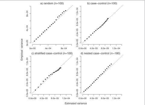
Figure 1 compares the average of the estimated standard error ofF1(t)ˆ in each simulation with the empirical stan-dard error at the 20 different times of observation in the four different scenarios with random censoring of 15 %. They were found to be very close in all scenarios, as expected.
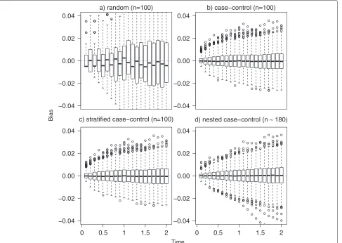
Figure 2 reports the distribution of bias in each one of the 1000 simulated samples under random (panel a), control (panel b), stratified (panel c) and nested case-control sampling (m=1, panel d). Bias fluctuates around 0 in each scenario, but it has more variability in the random sampling compared to other scenarios, resulting also in a higher mean value of absolute bias over the B simulations (still always lower than 0.2 %). The lower per-formance of the estimator in the first scenario is due to the fact that random sampling is not a convenient design in the simulated setting. In fact, in phase I cohort we expect around 90 events of type 1 (incidence of 9 % and sample size of 1000), thus if we randomly sample 100 sub-jects from the phase I cohort, we expect to observe only 9 events (in phase II sample). With such a small number of events, unbiasedness is in fact not sufficient to ensure a reasonable behaviour and to get enough information
on event incidence. To address this issue, the other study designs (scenarios 2, 3, and 4) are indeed thought to guar-antee to sample more events of type 1. Thus we recom-mend adopting efficient designs accounting for the event of interest. Relative and standardized biases were always lower than 6 % (data not shown). The mean square error, not shown, slightly increases with time, in fact variability is increasing in time (as confirmed by the empirical stan-dard error ofFˆ1(t)and by Fig. 2). The average length of the confidence interval was consistently increasing with time, ranging between 7 % and 12 % in the random sampling and between 2 % and 4 % in the case-control, stratified and nested case-control sampling (data not shown). This com-parison underscores the advantages of a careful selection of the subsample.
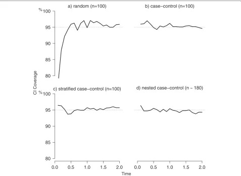
Figure 3 reports results on coverage for the random, case-control, stratified and nested case-control sampling. The coverage was very close to the nominal value of 95 %, ranging mostly within a minimum of 94 % and a maximum of 97 %, except for very early times in the random setting.
In the same setting, we also considered a longer follow-up time, t = 50, with around 500 events of type 1 expected in phase I sample (under no censoring), and confirmed the performance of our estimator in a scenario with higher variability, with similar results for the different sampling schemes (data not shown).
Motivating examples
Fig. 1Estimated and empirical variances. Comparison between estimated and empirical variance under random (panela), case-control (panelb), stratified (panelc) and nested case-control sampling (m=1, paneld). For the first three scenarios a sample size of 100 was used, while in the nested case-control sampling a mean of 180 subjects was considered. Data were subject to a random censoring of 15 % (plus administrative censoring). Dashed lines represent the main bisector corresponding to the equality between estimated and empirical reference
treatment protocols (Table 1). Strata were not defined based on the competing event death due to toxicity- 58 events - for efficiency reasons given that the event of interest was relapse. Patients were sampled at random without replacement from the 6 strata, with the sampling from each stratum conducted independently (stratified sampling) and with higher probability in the more infor-mative strata according to an optimal design [13]. The full cohort of 1999 patients represents the phase I sample, for which clinical information are available, while genotype is ascertained in the phase II sample only (n=601).
Relapses were classified according to the site, in par-ticular we distinguished relapses involving bone-marrow (BM) from the others (extramedullary). We estimated the crude incidence of BM relapse by GST-T1 deletion using (6) and (10) and found higher relapse incidence for patients with GST-T1 deletion, with 5-year crude inci-dence of 19.3 % (95 % CI: 13.4−27.7 %) versus 12.4 % (95 % CI: 10.7−14.4 % for non deleted patients, Fig. 4 panel a).
This was derived accounting for the competing risk of other sites of relapse as well as for death due to toxicity.
We report here the R code used to compute these estimates:
library(survey)
d.std<-twophase(id=list(˜ upn,˜ upn), subset=˜ !is.na(GST_T), strata=list
(NULL, ˜ interaction(rel,elfin)),data=dat) GSTse<-svycr(Surv(time,event>0)˜ GST_T, etype=“BMrelapse”,d.std,se=TRUE)
The twophase function in the survey package describes the design and produces a survey object [32]. Thesvycrfunction, available at [33], performs the esti-mate of crude incidence by the influence approach and uses 3 variables: time is the time of event,event the censoring indicator (1 if an event of any type is observed
and 0 otherwise) and BMrelapse indicates whether a
BM relapse is observed or not. Details on the survey
Fig. 2Bias distribution. Distribution of bias in the 1000 simulated samples under random (panela), case-control (panelb), stratified (panelc) and nested case control sampling (m=1, paneld). For the first three scenarios a sample size of 100 was used, while in the nested case-control sampling a mean of 180 subjects was considered. Data were subject to a random censoring of 15 % (over administrative censoring). The box represent the first and third quartile, the black line the median and the empty dots represent outliers defined as bias more than 1.5 times the interquartile range above the third quartile (or more than 1.5 times the interquartile range below the first quartile). Dotted lines represent the reference for bias (bias equal to 0)
The right panel of Fig. 4 represents the incidence of extramedullary relapses by GST-T1 showing that the dif-ference in relapse incidence between GST-T1 deleted and other patients is mainly due to relapse involving the BM, that represents the most relevant type of relapse in child-hood ALL. A Cox model adapted for two-phase design [14], when applied to the cause specific hazard of BM relapse, gives an hazard ratio (HR) of 1.53 (95 % CI 0.98– 2.37) for GST-T1 deleted patients versus non deleted; after adjusting for relevant factors (treatment protocol, gender, age), the HR dropped to 1.38 (95 % CI 0.90–2.13). For extramedullary relapses the HR was 1.22 (95 % CI 0.60– 2.49). Of note, in order to compare patients with and with-out deletion of the GST-T1 gene, we used a cause-specific model, thus we actually compared the cause-specific haz-ard of relapse. In fact, a subdistribution model accounting for the two-phase design is not available. This would be useful to compare the actual incidences of relapse in the
two groups, however the cause-specific model is still very useful to address the impact of the genotype on relapse by an aetiological point of view.
Fig. 3Coverage of confidence intervals. Simulation results for the coverage of confidence intervals (CI) under random (panela), case-control (panel b), stratified (panelc) and nested case-control sampling (m=1, paneld). For the first three scenarios a sample size of 100 was used, while in the nested case control sampling a mean of 180 subjects was considered. Data were subject to a random censoring of 15 % (over administrative censoring). Dotted lines represent the reference for CI coverage (nominal 95 %)
be dead, one approach to obtain outcomes estimates has been to identify a numerically small, but random, sample of those who are lost [15], intensively seeking their out-comes, and using them to correct outcomes among the lost.
Table 1Distribution of phase I (Ns) and II (ns) samples in the 6
strata and sampling fractions expressed as percentages in parenthesis for Phase II
Treatment protocol Standard Medium High
ns/Ns(%) Total No relapse 54/487 (11.1) 193/987 (19.6) 109/219 (49.8) 356/1693 Relapse 21/28 (75.0) 147/186 (79.0) 77/92 (83.7) 245/306 Total 75/515 340/1173 186/311 601/1999
To illustrate, a cohort of 13,321 HIV-infected adult patients, who initiated ART treatment, were followed from ART initiation to either death, disengagement or administrative database closure (see Fig. 5). Among them, 2451 patients were lost to follow-up [35], defined as not being seen at the clinic for at least 90 days (after the last return visit). A tracker went into the community to determine the outcome of a random subsample of 428 among the 2451 lost patients and got information on 306 patients (110 patient were found to be in care in other clinics, 80 died while in care and 116 were found to be not treated/disengaged) [12]. The 10,870 patients no lost to follow-up and the 306 tracked patients can been considered as the second phase sample of the whole cohort, stratified on lost to follow-up.
Fig. 4Crude cumulative incidence of relapse in ALL data. Panelareports the crude cumulative incidence estimate of relapse involving the bone marrow in patients with normal (estimate and confidence limits reported with solid lines) and deleted (dashed lines) GST-T1 gene. Panelbreports the crude cumulative incidence estimate of relapse in extramedullary sites in patients with normal (solid lines) and deleted (dashed lines) GST-T1 gene
sampling probability 306/2451, while the other 10,870 had sampling weight one. The crude incidence estimate of dis-engagement is reported in Fig. 6, the curve starts to rise after 90 days from ART start, that is the earliest possible time of disengagement, by definition. At 1 year, disengage-ment resulted 6.8 % (CI 95 % 5.7–8.2 %). This was subject to a strong influence of the competing event death in care that resulted 7.7 % (CI 95 % 6.8–8.9 %) at 1 year. A
naïve (but less expensive) approach to deal with infor-mative censoring would be to treat all lost patients as events or, contrarily, as censored observations. We plotted the two corresponding curves in Fig. 6, obtaining esti-mates of crude incidence at 1 year since ART treatment of 18.5 % and 0.2 %, respectively. We can consider that the true incidence will lie between these two estimates (that are however quite far in this context), as in fact it does
Fig. 6Crude cumulative incidence of disengagement in the HIV data. Crude cumulative incidence of disengagement of the 13,321 HIV patients who initiated ART treatment (black line) with confidence intervals (dashed lines). In the bottom part of the plot the number of patients at risk in time is reported (weighed to represent the whole cohort of 13,321). The dashed grey lines report the crude cumulative incidence of disengagement computed by treating all lost patients as event or censored observation, respectively
the estimate we got by tracking a random sample of lost patients and using the proposed estimator.
Availability of supporting data
The R code to compute the proposed estimate of crude cumulative incidence is available at [33]. The results of simulations presented in the Simulations section and the related code are also available at [33].
Conclusions
We have derived an estimator for cumulative incidence of events based on the subdistribution hazard accounting for competing risks under a general sampling design from an infinite target population. The estimator shows good per-formance in simulations under different scenarios and the variance, derived by the influence function of the subdis-tribution hazard and the Horvitz-Thompson theory, was very close to the empirical variance, therefore we expect it to be very close to the one obtainable by replicate weights (e.g. bootstrap) [7]. Confidence intervals, derived on the log scale, provided good coverage in simulations, but alter-native confidence intervals might also be considered such as the complementary log-log transformation [36]. The proposed estimator was used to estimate incidence of relapse by genotype in a cohort of childhood ALL patients,
where the genotype was ascertained only on a subsam-ple of the cohort chosen by an optimal sampling approach based on relapse as the event of interest. Interestingly, we can also analyze the incidence of the competing event (toxic death) or of the combined endpoint (relapse or toxic death), but the efficiency could be lower unless the sub-sampling is adapted to this new endpoint by including a further strata on toxic death in the sampling process. This is particularly important since toxic death is a rare event in this context. We should also remember to avoid random sampling when the event of interest is rare, as discussed in the Simulations section.
how the proposed estimator could be applied also in the presence of missing data.
The code to compute this estimate has been developed in R software [31] under thesurveypackage [32] and is available at [33]. The survey package is a flexible package for complex surveys including also two-phase studies. It provides flexible functions to describe the design of the study and to derive sampling fraction accordingly. The package includes functions to estimate survival and to perform a weighted Cox model with standard error prop-erly adjusted for the design and with the possibility to use general weights, as calibrated weights. Our function takes advantage of the facilities of the package (see an example of use in Genotype ascertained on a subset of a clinical trial cohort).
In order to recover the representativeness of the sub-cohort (phase II) for the entire sub-cohort, we used weights related to the inverse of the probability to be sampled, similarly to the weights of Barlow for case-cohort studies [38]. More general weights can be used, such as calibration weights [7, 39, 40]. The use of calibration weights is advan-tageous when there is availability of phase I variables that are strongly related to the additional variables ascertained in phase II. This would provide results more representa-tive of phase I data and increase precision. When phase II variables are common genetic polymorphisms, as in our first example, it is unlikely to find any strong rela-tion between phase I and II variables, therefore no big advantage would be expected by calibration.
The estimator can also be extended to a situation where an individual may move among a finite number of states to estimate the Aalen-Johansen probabilities of transition among each state in a multistate framework [41] in the presence of general sampling design.
In order to derive a model-based estimate of incidence (adjusted for possible covariates) two main approaches have been followed in the context of competing risk, the first one based on the cause-specific hazard inspired by Benichou and Gail [16, 42, 43] and the other one based on the subdistribution hazard [19, 44]. The crude cumu-lative estimator developed by Kovalchik and Pfeiffer [45] for two-phase studies for finite population follows the first approach, and the Cox model for two-phase designs [14] could be used to extend it for infinite population. Under this model we can estimate the effect of a covari-ate on the cause-specific hazard to address its impact on the event by an aetiological point of view. However it is well known that this does not reflect the impact of the variable on the crude cumulative incidence. The lat-ter effect, even if affected by the incidence of the other competing events, could still be of interest for a public health prospective. Future work will concern the devel-opment of a regression model to assess the effect of a covariate on the crude cumulative incidence. The Fine
and Gray regression model [19] could be extended to complex sampling by weighting the estimating function of the parameter of interest and working out their influence function.
A Appendix
A.1 Derivation of the risk set forTk∗
The risk set for the usual survival timeTatsis commonly obtained in standard analysis by counting the observed times greater thens. It can be also written as:
ˆ
Y·(s)= ˆP(T>s−)P(Cˆ >s−)= ˆY·(0)S(sˆ −)G(sˆ −) (12)
whereGˆ(s)is the probability to be free of censoring up to
sand is estimated considering censored observations as events and viceversa according to (3). This can proved also in the case of a two-phase design by the following:
ˆ
Y·(0)Sˆ(s−)· ˆG(s−)= ˆY·(0)
u<s
1−Nˆ··(du) ˆ Y·(u)
·
u<s
1− Nˆ
c ·(du)
ˆ
Y·(u)− ˆN··(du)
=
= ˆY·(0)
u<s
ˆ
Y·(u)−[Nˆ··(du)+ ˆN·c(du)] ˆ
Y·(u)
=
= ˆY·(0)
u<s
ˆ Y·(u+)
ˆ Y·(u) =
ˆ Y·(0)Yˆ·(s)
ˆ Y·(0) =
=
N
i=1
[ξiYi(s)/πi]
(13)
whereNˆ·c(t) = Ni=1[ξiI(Xi≤t,i=0)/πi] denotes the number of censoring up to timetandNˆ··(t)=ni=1Nˆi·(t) the total count of events observed up to timet.
The derivation of the risk set forTk∗atscan be obtained by:
ˆ
Y·∗k(s)= ˆP Tk∗>s−Pˆ(C>s−)= ˆY·(0)·
1− ˆFk(s−)
ˆ G(s−)=
= ˆY·(0)·
⎡
⎣Sˆ(s−)+ l=k ˆ Fl(s−)
⎤
⎦· ˆG(s−)=
= ˆY·(s)+ ˆY·(0)· l=k ˆ
Fl(s−)· ˆG(s−)
(14)
By writingFˆl(s−) as empirical cumulative distribution functionFˆl(s−) = Yˆ·1(0)
N i=1πξii
I(Xi≤s−;εi=l)
ˆ G(Xi−∧s−)
ˆ
Y·∗k(s)= ˆY·(s)+ l=k
N
i=1 ξi πiI(Xi≤
s−;εi=l) ˆ G(s−) ˆ
G Xi−∧s−
(15)
that can be simplified to
N
i=1 ξi πi
Yi(s)+ N i=1 ξi πi ⎡ ⎣
l=k
Nil(s−)· ˆG s−|Xi− ⎤⎦
(16)
that is equivalent to (4).
The first summation estimates the usual total num-ber of subjects at risk at s, where the condition Xi = min(Ti,Ci) ≥ s is satisfied. This in fact implies min(Tki∗,Ci)≥s, i.e. being at risk forT implies being also at risk forTk∗. The second summation estimates the num-ber of subjects who had other events befores, satisfying the conditionXi = min(Ti,Ci) < s,i = 1 andεi = k which impliesTki∗ = ∞>sand completes the number at risk atsforTk∗. While the first part is exposed to censor-ing, the contribute of each subject observed to fail of cause
l = k, l=kNil(s−), would remain equal to 1 up to∞, thus ignoring possible censoring, given thatCiis (usually) not observable ifTi<Ci. A possible way to deal with this inconsistency is to mimic the presence of random censor-ing actcensor-ing on the infinite times, by weightcensor-ing the unitary contributionsl=kNil(s−)by the estimate Gˆ(s−|Xi−) of P(C >s−|C> Xi−)=G(s−|Xi), whereG(t)=P(C >t)
is estimated by Gˆ(t) = s≤t
1−
N
i=1ξiNic(ds)/πi
N
i=1ξiYi(s)/πi
, with
Nic(s) = I(Xi ≤ s,i = 0). This weight assumes value
1 before Xi and decreases afterword according to the
censoring distribution.
Of note, an alternative expression for Yˆ·∗k(s) derives
substitutingYˆ·(0)G(sˆ −)= ˆYˆ·(s)
S(s−) from (12) in (14):
ˆ
Y·∗k(s)= ˆY·(0)G(sˆ −)·
1− ˆFk(s−)
= ˆY·(s)
1− ˆFk(s−)
ˆ S(s−)
(17)
This shows asYˆ·(s) is upweighted by a multiplier that gets greater as the action of competing events gets larger, accounting for the fact that subjects that experienced events of typel=kwill never experience eventkas first.
A.2 Proof of equivalence (7)
The equality between the cumulative incidence of the arti-ficial variableT∗in (6) and the Aalen-Johansen type esti-mator (that for the purpose of this proof will be denoted asFˆkAJ(t)) holds true if and only if,∀t:
ˆ FkAJ(t)=
t
0 ˆ S(s−)ˆ
k(ds)=1− s≤t
1− ˆ∗k(ds)
= ˆFk(t)
(18)
which can be proved by induction. Both quantities are step functions, changing value at each occurrence of type
k events. At the timetwhere the first event of typekis observed,ˆk(dt)= ˆ∗k(dt)being from (4)Yˆ·(t)= ˆY·∗k(t). If this was the first event overall, thenS(ˆ 0)=1 and Eq. 18 is satisfied, otherwiseFˆkAJ(t) =[1−1/Yˆ·(0)]·1/[Yˆ·(0)− 1]=1/Yˆ·(0)=1−[1−1/Yˆ·(0)]= ˆFk(t).
Now, assuming that (18) holds true for a givent−, this impliesFˆkAJ(t)= ˆFk(t)if and only if, from (18):
ˆ
FkAJ(t−)+ ˆS(t−)ˆk(dt)=1−(1− ˆFk(t−))
1− ˆ∗k(dt)
and using the equality att−:
ˆ
Fk(t−)+ ˆS(t−)ˆk(dt)= ˆFk(t−)+
1− ˆFk(t−)
ˆ ∗
k(dt) ˆ
S(t−)ˆk(dt)=
1− ˆFk(t−)
ˆ ∗k(dt)
ˆ k(dt)=
1− ˆFk(t−) ˆ
S(t−) ˆ ∗ k(dt)
ˆ Nk(dt)
ˆ Y·(t) =
1− ˆFk(t−) ˆ S(t−)
ˆ Nk(dt)
ˆ Y·∗k(t)
ˆ
Y·∗k(t)= ˆY·(t)·1− ˆFk(t −) ˆ S(t−)
That is proved by (17).
A.3 Weak convergence ofˆ∗k(t)
Lin showed that the normalised Horvitz-Thompson estimators of the number of events √NNˆ·(t)−N·(t),
number at risk √N
ˆ
Y·(t)−Y·(t)
, cumulative hazard √
N[(t)ˆ −(t)] and survival function√N
ˆ
S(t)−S(t)
(and analogously √N
ˆ
G(t)−G(t)) are asymptotically multivariate zero-mean normal [14]. Firstly, we con-centrate on the normalised Horvitz-Thompson
esti-mators of the modified at risk process:
√
NYˆ·∗k(t)−Y·∗k(t)=√NNi=1ξi−πi
πi Y
∗ ·k(t)=
√ NNi=1 ξi−πi
πi Y·k(t)+
√
NNi=1ξi−πi
πi
√ N N i=1 ⎡ ⎣ξi
πi·
l=k
Nil(t−)Gˆ(t−|Xi)−
l=k
Nil(t−)Gˆ(t−|Xi)
⎤
⎦=
=√N N
i=1 ⎡ ⎣Gˆ(t−|Xi)
⎧ ⎨ ⎩πξii
l=k
Nil(t−)−
l=k Nil(t−)
⎫ ⎬ ⎭ ⎤
⎦=
=√N ⎡ ⎣Gˆ(t−|Xi)
⎧ ⎨ ⎩
l=k ˆ N·l(t−)−
l=k N
i=1 Nil(t−)
⎫ ⎬ ⎭ ⎤
⎦=
=√N t−
0
ˆ G(s−|Xi)
⎧ ⎨ ⎩
l=k ˆ
N·l(ds−)−
l=k N
i=1
Nil(ds−)
⎫ ⎬
⎭=
=√N t−
0
G(t−|Xi)
⎧ ⎨ ⎩
l=k ˆ
N·l(ds−)−
l=k N
i=1
Nil(ds−)
⎫ ⎬
⎭+
+op(1)
that using Lemma 1 in [14] also converges to a zero-mean Gaussian process.
We want to prove that also √N
ˆ ∗
k(t)−∗k(t)
= √
N˜∗k(t)−∗k(t) + √Nˆ∗k(t)− ˜∗k(t) converges
to a zero-mean normal, where ˜∗k(t) represents the crude cumulative incidence estimator that we would have obtained if complete information(Xi,iεi,Zi)was known for all the subjects in phase I sample (i = 1. . .N) [18]. Fine and Gray proved that the first term converges weakly to a zero-mean Gaussian process [19].
The second term results:
√
N
ˆ
∗k(t)− ˜∗k(t)
=√N
t
0
ˆ
Nk(ds)
ˆ
Y·∗k(s) −
t
0 Nk(ds)
Y·∗k(s)
=
=√N
t
0
ˆ
Nk(ds)
ˆ
Y·∗k(s) −
t
0 Nk(ds)
Y·∗k(s) +
t
0 Nk(ds)
ˆ
Y·∗k(s) −
t
0 Nk(ds)
ˆ
Y·∗k(s)
=
=√N
⎡ ⎣ t
0
ˆ
Nk(ds)−Nk(ds)
ˆ
Y·∗k(s) −
t
0 Nk(ds)
ˆ
Y·∗k(s)−Y·∗k(s)
ˆ
Y·∗k(s)Y·∗k(s)
⎤ ⎦.
It then follows that also√Nˆ∗k(t)− ˜∗k(t)converges weakly to a zero-mean Gaussian process.
A.4 Influence function forˆ∗k(t)
The estimatorˆ∗k(t)can be expressed as a differentiable functiongof the estimated total number of events of type
kand total number at risk forT∗up tot:
ˆ
∗k(t)=g(Nˆ·k(dt),Yˆ·∗k(t))= t
0 ˆ N·k(ds)
ˆ Y·∗k(s) =
= t
0 N
i=1ξi·Nik(ds)wi N
i=1ξi·Yik∗(s)wi (19)
where wi = 1/πi andξi indicates whether subject i is withdrawn in the phase II sample.
The difference between the true and estimated cumu-lative hazard can be expressed as a sum of influence functions:ˆ∗k(t)−∗k(t)=iN=1z∗ik+o(1/√N), wherez∗ik
is the influence function of theithsubject. Demnati and Rao [27] proved that we can express the influence
func-tion of subjectiasz∗ik(t)= ∂g
ˆ
N·k(dt),Yˆ·∗k(t)
∂wi . The influence
function ofˆ∗k(t)of theithsubject can thus be derived as:
z∗ik(t)= t
0
Nik(ds)Yˆ·∗k(s)− ∂Yˆ·∗k(s)
∂wi Nˆ·k(ds)
ˆ
Y·∗k(s)2 (20)
BeingYˆ·∗k(s) = Ni=1ξiwi ·
Yi(s)+I(Xi≤s −;ε
i=k)G(sˆ −)
ˆ G(X−
i ∧s−)
and beingG(s)ˆ =u≤s
1−
N
i=1ξiNic(du)/πi
N
i=1ξiYi(u)/πi
, the
deriva-tive ofYˆ·∗k(s)with respect towiresults:
∂Yˆ·∗k(s) ∂wi =
∂
ξiwi·
Yi(s)+ I(Xi≤s −;ε
i=k)G(sˆ −)
ˆ GXi−∧s−
+
j=i ξjwj·
Yj(s)+I(Xj≤s −;ε
j=k)G(sˆ −)
ˆ G
Xj−∧s−
∂wi =
=ξiYi(s)+ξi ∂
wiI(Xi≤s
−;ε
i=k)G(sˆ −)
ˆ GX−i∧s−
∂wi +
∂
j=i
ξjwjI(Xj≤s−;εj=k)G(sˆ −)
ˆ G
Xj−∧s−
∂wi =
=ξiYi(s)+ξi
I(Xi≤s−;εi=k)Gˆ(s−) ˆ
G Xi−∧s− + N
j=1
ξjwjI(Xj≤s−;εj=k)∂w∂ i
⎡
⎣ Gˆ(s−) ˆ G
X−j ∧s−
⎤ ⎦.
Please note that the last addendum accounts for the fact thatGˆ(t)is estimated using information of subjecti. For
v≤u:
∂ ∂wi
ˆ G(u)
ˆ G(v)
=Gˆ(u)
u 0
dNc
i(s)−ˆλc(s)Yi(s)
ˆ
Y·(s) Gˆ(v)− ˆG(v) v
0 dNc
i(s)−ˆλc(s)Yi(s)
ˆ
Y·(s) Gˆ(u) ˆ
G(v)2 =
=Gˆ(u)Gˆ(v) u
v+ dNc
i(s)−ˆλc(s)Yi(s)
ˆ Y·(s) ˆ
G(v)2 =
ˆ
G(u)vu+dN
c
i(s)−ˆλc(s)Yi(s)
ˆ Y·(s) ˆ G(v)
(22)
where the superscriptcindicates the quantities related to the censoring process, i.e.Nic(u)= I(Xi ≤u,i =0)is the indicator of censoring for subjectiup to timeuandλˆc(u)= ˆN·c(du)/Yˆ·(u)the instantaneous hazard of censoring. The derivative ofYˆ·∗k(u)becomes:
∂Yˆ·∗k(s) ∂wi =
Yi(s)+I(Xi≤s−;εi=k)· ˆ G(s−) ˆ
G Xi−∧s−+ N
j=1
ξjwjI(Xj≤s−;εj=k) ˆ G(s−) ˆ G
Xj−∧s−
s
−
Xj
Nic(du)− ˆλc(u)Y i(u) ˆ
Y·(u)
(23)
Thus, the influence function ofˆ∗k(t)of theithsubject results:
z∗ik(t)=
t0
Nik(ds)Yˆ·∗k(s)− ˆN·k(ds)
Yi(s)+I(Xi≤s −;ε
i=k)G(sˆ −)
ˆ GX−i∧s−
+N j=1
ξjwjI(Xj≤s−;εj=k)G(sˆ −)
ˆ G
Xj−∧s−
s− Xj
Nc
i(du)−ˆλc(u)Yi(u)
ˆ Y·(s)
ˆ
Y·∗k(s)2 =
=
t0
Nik(ds)− ˆ∗k(ds)
Yi(s)+I(Xi≤s
−;εi=k)G(sˆ −) ˆ
GXi−∧s−
+N j=1
ξjI(Xj≤s−;εj=k)G(sˆ −)
πjGˆ
X−j ∧s−
s− Xj
Nc
i(du)−ˆλc(u)Yi(u)
ˆ Y·(u)
ˆ Y·∗k(s)
(24)
wherewj = 1/πj. By definingMci(s,t) = t
s
Nic(du)−ˆλc(u)Yi(u)
ˆ
Y·(u) as the influence function of subjection censoring,vj = ξj
πj
l=kNjl(s−)G(sˆ −|X−j ), andMik(s)=
Nik(s)− ˆ∗k(s)Yik∗(s)
/Yˆ·∗k(s). Thus it can be reduced as:
z∗ik(t)=
t0
Nik(ds)− ˆ∗k(ds)Yik∗(s)− ˆ∗k(ds) N j=1 ξj πj
l=kNjl(s−)Gˆ
s−|Xj−
Mci Xj,s−
ˆ
Y·∗k(s) =
=
t0
Mik(ds)− ˆ ∗ k(ds) N j=1
vjMci Xj,s−
Abbreviations
ALL: Acute lymphoblastic leukemia; ART: Antiretroviral therapy;
BM: Bone-marrow; CI: Confidence interval; GST-T1: Glutathione S-transferase-θ; HR: Hazard ratio.
Competing interests
The authors declare that they have no competing interests.
Authors’ contributions
PR performed the theoretical derivation, analyses and simulation studies and drafted the manuscript. LA, DVG, MGV contributed to the analyses and to the manuscript. All authors read and approved the final manuscript.
Acknowledgements
The authors thank Thomas Lumley for useful comments, Raffaella Franca and Marco Rabusin for the ALL data and Jeff Martin and Elvin Geng for the HIV data. PR was supported by the grant SIR RBSI14LOVD of the Italian Ministry of Education, University and Research. This research was partially supported by AIRC (2013-14634, MGV) and by NIH (U01 AI069911).
Author details
1Center of Biostatistics for Clinical Epidemiology, School of Medicine and
Surgery, University of Milano-Bicocca, via Cadore 48, 20900 Monza, Italy. 2Department of Epidemiology and Biostatistics, University of California, San
Francisco, California.
Received: 17 September 2015 Accepted: 17 December 2015
References
1. Neyman J. Contribution to the theory of sampling human populations. J Am Stat Assoc. 1938;33(201):101–16.
2. Borgan Ø, Samuelsen SO. A review of cohort sampling designs for Cox’s regression model: Potentials in epidemiology. Norsk Epidemiol. 2003;13: 239–48.
3. Prentice RL. A case-cohort design for epidemiologic cohort studies and disease prevention trials. Biometrika. 1986;73(1):1–11.
4. Samuelsen SO. A psudolikelihood approach to analysis of nested case-control studies. Biometrika. 1997;84(2):379–94.
5. Langholz B, Borgan Ø. Counter-matching: a stratified nested case-control sampling method. Biometrika. 1995;82(1):69–79.
6. Rudolph KE, Gary SW, Stuart EA, Glass TA, Marques AH, Duncko R, et al. The association between cortisol and neighborhood disadvantage in a US population-based sample of adolescents. Health Place. 2014;25:68–77. 7. Lumley TS. Complex Surveys: A Guide to Analysis Using R. 1st ed. Inc JWS, editor. Wiley Series in Survey Methodology. Hoboken, New Jersey: John Wiley & Sons; 2010.
8. Breslow N, Lumley T, Ballantyne C, Chambless L, Kulich M. Using the Whole Cohort in the Analysis of Case-Cohort Data. Am J Epidemiol. 2009;169(11):1398–405.
9. Anderson GL, Manson J, Wallace R, Lund B, Hall D, Davis S, et al. Implementation of the women’s health initiative study design. Ann Epidemiol. 2003;13(9, Supplement):S5—17.
10. Fried LP, Borhani NO, Enright P, Furberg CD, Gardin JM, Kronmal RA, et al. The Cardiovascular Health Study: design and rationale. Ann Epidemiol. 1991;1(3):263–76.
11. Franca R, Rebora P, Basso G, Biondi A, Cazzaniga G, Crovella S, et al. Glutathione S-transferase homozygous deletions and relapse in childhood acute lymphoblastic leukemia: a novel study design in a large Italian AIEOP cohort. Pharmacogenomics. 2012;13(16):1905–16. 12. Geng E, Emenyonu N, Bwana M, Glidden D, Martin J. Sampling-based
approach to determining outcomes of patients lost to follow-up in antiretroviral therapy scale-up programs in Africa. JAMA. 2008;300(5): 506–7. Available from: http://dx.doi.org/10.1001/jama.300.5.506. 13. Rebora P, Valsecchi MG. Survival estimation in two-phase cohort studies
with application to biomarkers evaluation. Stat Methods Med Res. 2014. in press. doi:10.1177/0962280214534411.
14. Lin DY. On fitting Cox’s proportional hazards models to survey data. Biometrika. 2000;87(1):37–47.
15. Frangakis CE, Rubin DB. Addressing an idiosyncrasy in estimating survival curves using double sampling in the presence of self-selected right censoring. Biometrics. 2001;57(2):333–42.
16. Borgan Ø. Estimation of covariate-dependent Markov transition probabilities from nested case-control data. Stat Methods Med Res. 2002;11(2):183–202.
17. Aalen OO, Borgan Ø, Fekjær H. Covariate adjustment of event histories estimated from Markov chains: the additive approach. Biometrics. 2001;57(4):993–1001.
18. Gray RJ. A class of K-sample tests for comparing the cumulative incidence of a competing risk. The Annals of Statistics. 1988;16(3):1141–54. 19. Fine JP, Gray RJ. A proportional hazards model for the subdistribution of
a competing risk. J Am Stat Assoc. 1999;94(446):496–509.
20. Antolini L, Biganzoli EM, Boracchi P. Crude cumulative incidence in the form of a Horvitz-Thompson like and Kaplan-Meier like estimator. COBRA Preprint Series. 2006. 10 http://biostats.bepress.com/cobra/art10. 21. Särndal C, Swensson B. A general view of estimation for two phases of
selection with applications to two-phase sampling and nonresponse. Int Stat Rev. 1987;55(3):279–94.
22. Kang S, Cai J. Marginal hazards model for case-cohort studies with multiple disease outcomes. Biometrika. 2009;96(4):887–901.
23. Marubini E, Valsecchi MG. Analysing survival data from clinical trials and observational studies. Chichester, England: Wiley-Interscience; 2004. 24. Bernasconi D, Antolini L. Description of survival data extended to the
case of competing risks: a teaching approach based on frequency tables. Epidemiol Biostat Public Heal. 2013;11(1):. e8874–1:e8874–10.
25. Satten GA, Datta S. The Kaplan-Meier estimator as an
inverse-probability-of-censoring weighted average. Am Stat. 2001;55(3): 207–10.
26. Breslow NE, Wellner JA. Weighted likelihood for semiparametric models and two-phase stratified samples, with application to cox regression. Scand J Stat. 2007;34(1):86–102.
27. Demnati A, Rao JNK. Linearization variance estimators for model parameters from complex survey data. Surv Methodol. 2010;36:193–201. 28. Breslow NE, Lumley T, Ballantyne CM, Chambless LE, Kulich M.
Improved Horvitz–Thompson estimation of model parameters from two-phase stratified samples: applications in epidemiology. Stat Biosci. 2009;1(1):32–49.
29. Horvitz DG, Thompson DJ. A generalization of sampling without replacement from a finite universe. J Am Stat Assoc. 1952;47(260):663–85. 30. de Wreede LC, Fiocco M, Putter H. mstate: An R Package for the Analysis
of Competing Risks and Multi-State Models. J Stat Softw. 2011;38(7):1–30. Available from: http://www.jstatsoft.org/v38/i07/.
31. R Core Team. R: A Language and Environment for Statistical Computing. Vienna, Austria: R Foundation for Statistical Computing; 2014. Available from: http://www.R-project.org.
32. Lumley T. Analysis of complex survey samples. J Stat Softw. 2004;9(8):1–19. 33. Rebora P. R code to estimate crude incidence in two-phase designs. 2015.
Accessed: 2015-10-27. http://dx.doi.org/10.6070/H4F18WRG. 34. Tsiatis AA. A nonidentifiability aspect of the problem of competing risks.
Proc Natl Acad Sci U S A. 1975;72(1):20–2.
35. Geng EH, Glidden DV, Bwana MB, Musinguzi N, Emenyonu N, Muyindike W, et al. Retention in care and connection to care among HIV-infected patients on antiretroviral therapy in Africa: estimation via a sampling-based approach. PLoS One. 2011;e21797:7.
36. Glidden DV. Robust inference for event probabilities with Non-Markov event data. Biometrics. 2002;58(2):361–68.
37. Lin DY, Ying Z. Cox regression with incomplete covariate measurements. J Am Stat Assoc. 1993;88:1341–9.
38. Barlow W, Ichikawa L, Rosner D, Izum iS. Analysis of case-cohort designs. J Clin Epidemiol. 1999;52(12):1165–72.
39. Scott AJ, Wild CJ. Fitting regression models with response-biased samples. Can J Stat. 2011;39(3):519–36.
40. Rudolph KE, Diaz I, Rosenblum M, Stuart EA. Estimating population treatment effects from a survey sub-sample. Am J Epidemiol. 2014;180: 737–48.
41. Aalen OO, Johansen S. An empirical transition matrix for
42. Benichou J, Gail MH. Estimates of absolute cause-specific risk in cohort studies. Biometrics. 1990;46(3):813–26. Available from: http://www.jstor. org/stable/2532098.
43. Langholz B, Borgan Ø. Estimation of absolute risk from nested case-control data. Biometrics. 1997;53(2):767–74.
44. Wolkewitz M, Cooper BS, Palomar-Martinez M, Olaechea-Astigarraga P, Alvarez-Lerma F, Schumacher M. Nested case-control studies in cohorts with competing events. Epidemiology. 2014;25(1):122–5.
45. Kovalchik S, Pfeiffer R. Population-based absolute risk estimation with survey data. Lifetime Data Anal. 2014;20(2):252–75.
46. Jewell NP, Lei X, Ghani AC, Donnelly CA, Leung GM, Ho LM, et al. Non-parametric estimation of the case fatality ratio with competing risks data: an application to Severe Acute Respiratory Syndrome (SARS). Stat Med. 2007;26(9):1982–98.
• We accept pre-submission inquiries
• Our selector tool helps you to find the most relevant journal
• We provide round the clock customer support
• Convenient online submission
• Thorough peer review
• Inclusion in PubMed and all major indexing services
• Maximum visibility for your research Submit your manuscript at
www.biomedcentral.com/submit