Assessment of fit of item response
theory models used in large‑scale
educational survey assessments
Peter W. van Rijn
1, Sandip Sinharay
2*, Shelby J. Haberman
3and Matthew S. Johnson
4Introduction
Several large-scale educational survey assessments (LESAs) such as the United States’ National Assessment of Educational Progress (NAEP), the International Adult Literacy Study (IALS; Kirsch 2001), the Trends in Mathematics and Science Study (TIMSS; Mar-tin and Kelly 1996), and the Progress in International Reading Literacy Study (PIRLS; Mullis et al. 2003) involve the use of item response theory (IRT) models for score-report-ing purposes (e.g., Beaton 1987; Mislevy et al. 1992; Von Davier and Sinharay 2014).
Standard 4.10 of the Standards for Educational and Psychological Testing (American Educational Research Association 2014) recommends obtaining evidence of model fit when an IRT model is used to make inferences from a data set. In addition, because of the importance of the LESAs in educational policy-making in the U.S. and abroad, it is essential to assess the fit of the IRT models used in these assessments. Although several researchers have examined the fit of the IRT models in the context of LESAs (for exam-ple, Beaton 2003; Dresher and Thind 2007; Sinharay et al. 2010), there is a substantial scope of further research on the topic (e.g., Sinharay et al. 2010).
This paper suggests two types of residuals to assess the fit of IRT models used in LESAs. One among them can be used to assess item fit and the other can be used to
Abstract
Latent regression models are used for score-reporting purposes in large-scale educa-tional survey assessments such as the Naeduca-tional Assessment of Educaeduca-tional Progress (NAEP) and Trends in International Mathematics and Science Study (TIMSS). One component of these models is based on item response theory. While there exists some research on assessment of fit of item response theory models in the context of large-scale assessments, there is a scope of further research on the topic. We suggest two types of residuals to assess the fit of item response theory models in the context of large-scale assessments. The Type I error rates and power of the residuals are computed from simulated data. The residuals are computed using data from four NAEP assess-ments. Misfit was found for all data sets for both types of residuals, but the practical significance of the misfit was minimal.
Keywords: Generalized residual, Item fit, Residual analysis, Two-parameter logistic model
Open Access
© 2016 The Author(s). This article is distributed under the terms of the Creative Commons Attribution 4.0 International License (http://creativecommons.org/licenses/by/4.0/), which permits unrestricted use, distribution, and reproduction in any medium, provided you give appropriate credit to the original author(s) and the source, provide a link to the Creative Commons license, and indicate if changes were made.
RESEARCH
*Correspondence: ssinharay@pacificmetrics. com
2 Pacific Metrics Corporation,
assess other aspects of fit of these models. These residuals are computed for several sim-ulated data sets and four operational NAEP data sets. The focus in the remainder of this paper will mostly be on NAEP.
The next section provides some background, describing the current NAEP IRT model and the existing NAEP IRT model-fit procedures. The Methods section describes our suggested residuals. The data section describes data from four NAEP assessments. The Simulation section describes a simulation study that examined the Type I error rate and power of the suggested methods. The next section involves the application of the sug-gested residuals to the four NAEP data sets. The last section includes conclusions and suggestions for future research.
Background
The IRT model used in NAEP
Consider a NAEP assessment that was administered to students i,i=1, 2,. . .,N ,
with corresponding sampling weights Wi. The sampling weight Wi represent the
num-ber of students in the population that student i represents (e.g., Allen et al. 2001
pp. 161–225). Denote the p-dimensional latent proficiency variable for student i by θi=(θi1,θi2,. . .,θip)′. In NAEP assessments, p is between 1 and 5. Denote the vector of item scores for student i by yi=(yi′1,yi′2,. . .,yip′ )′, where the sub-vector yik contains the item scores yijk,j∈Jik, of student i to items (that are indexed by j) corresponding to the kth dimension/subscale that were presented to student i. For example, yik could be the scores of student i to the algebra questions presented to her on a mathematics test and θik could represent the student’s proficiency variable for algebra. Because of the use of matrix sampling (that refers to a design in which each student is presented only a subset of all available items) in NAEP assessments, the algebra questions administered to stu-dent i are a subset Jik of the set Jk of all available algebra questions on the test. The item scores yijk can be an integer between 0 and rjk >0, where rjk =1 for dichotomous items and an integer larger than 1 for polytomous items with three or more score categories.
Let βk denote the vector of item parameters of the items related to the kth subscale, and let β=(β′1,β′2,. . .,β′p)′. For item j in Jik, let fjk(y|θik,βk) be the probability given θik and βk that yijk =y, 0≤y≤rjk, and let
Then fk(yik|θik,βk) is the conditional likelihood of an examinee on the items corre-sponding to the k-th subscale. Because of the between-item multidimensionality of the items (that refers to each item measuring only one subscale; e.g., Adams et al. 1997) used in NAEP, the conditional likelihood for a student i given θi is given by
In Equation 2, the expressions fk(yik|θik,βk) are defined by the particular IRT model used for analysis, which is usually the three-parameter logistic (3PL) model (Birnbaum
1968) for multiple-choice items, the two-parameter logistic (2PL) model (Birnbaum (1)
fk(yik|θik,βk)=
j∈Jik
fjk(y|θik,βk).
(2) f(yi|θi,β)=
p
k=1
1968) for dichotomous constructed-response items, and the generalized partial-credit model (GPCM; Muraki 1992) for polytomous constructed-response items. Parame-ter identification requires some linear constraints on the item parameParame-ters β or on the regression parameters Ŵ and .
Associated with student i is a vector zi=(zi1,zi2,. . .,ziq) of background variables. It is assumed that yi and zi are conditionally independent given θi and, for some p by q matrix
Ŵ and some p by p positive-definite symmetric matrix , the latent regression assump-tion is made that
where Np denotes the p-dimensional normal distribution (e.g., Beaton 1987; Von Davier and Sinharay 2014). Let φ (θ;Ŵzi,�) denote the density at θ of the above normal distribution.
Weighted maximum marginal likelihood estimates may then be computed for the item parameters, the matrix Ŵ, and the matrix by maximizing the weighted log likelihood
The resulting estimates are βˆ =(βˆ′
1,. . .,βˆ ′
p), Ŵˆ, and ˆ. The model described by Eqs. 1 – 4 will henceforth be referred to as the “NAEP operational model” or the “NAEP model”. The model given by Eqs. 1 and 2 are often referred to as the “NAEP measurement model” or the “IRT part of the NAEP model”.
In this report, a limited version of the NAEP model is used where no background vari-ables are employed, and θi is assumed to have a multivariate normal distribution with means equal to 0 and constraints on the covariance matrix, so that the variances are equal to 1 if the covariances are all zero. Consideration of only this limited model allows us to focus on the fit of the IRT part (given by Eqs. 1 and 2) of the NAEP model rather than on the latent regression part (given by Eq. 3). If zi has a normal distribution, then this limited model is consistent with the general NAEP model. The suggested residu-als can be extended to the case in which background variables are considered. These extensions are already present in the software employed in the analysis in this paper. For example, residuals involving item responses and background variables can indicate whether the covariances of item responses and background variables are consistent with the IRT model. The extensions can also examine whether problems with residual behav-ior found when ignoring background variables are removed by including background variables in the model. This possibility is present if background variables that are not normally distributed are related to latent variables.
Existing tools for assessment of fit of the NAEP IRT model
The assessment of fit of the NAEP IRT model is more complicated than that of the IRT models used in other testing programs because of several unique features of NAEP. Two such major features are:
(3)
θi|zi ∼Np(Ŵzi,�),
(4) ℓ(β,Ŵ,�)=
N
i=1 Wilog
• Because NAEP involves matrix sampling, common model-fit tools such as the item-fit statistics of Orlando and Thissen (2000), which are appropriate when all items are administered to all examinees, cannot be applied without modification.
• Complex sampling involves both the sampling weights Wi and departures from
cus-tomary assumptions of independent examinees due to sampling from finite popula-tions and due to first sampling schools and then sampling students within schools.
However, there exist several approaches for assessing the fit of the NAEP IRT model. The primary model-fit tool used in the NAEP operational analyses is graphical item-fit analyses using residual plots and a related χ2-type item-fit statistic (Allen et al. 2001 p. 233) that provide guidelines for treating the items (such as collapsing categories of poly-tomous items, treating adjacent year data separately in concurrent calibration, or drop-ping items from the analysis). However, the null distribution1 of these residuals and of the χ2-type statistic are unknown (Allen et al. 2001 p. 233).
Differential item functioning (DIF) analyses are also used in NAEP operational analysis to examine one aspect of multidimensionality (Allen et al. 2001 p. 233). In addition, the difference between the observed and model-predicted proportions of students obtain-ing a particular score on an item (Rogers et al. 2006) are also examined in NAEP opera-tional analyses. However, to evaluate when a difference can be considered large enough, the standard deviation of the difference is not used. It will be useful to incorporate the variability in the comparison of the observed and predicted proportions. As will be clear later, our proposed approach addresses this issue.
Beaton (2003) suggested the use of item-fit measures involving weighted sums and weighted sums of squared residuals obtained from the responses of the students to each question of NAEP. Let Eˆijk be the estimated conditional expectation of yijk given zi based on the parameter estimates βˆ, Ŵˆ, and ˆ, and let σˆ
ijk be the corresponding estimated con-ditional standard deviation of yijk. Let us consider item j that measures the k-th subscale and let Kjk be the set of students i who were presented the item. Beaton’s fit indices are of the forms
The bootstrap method (e.g., Efron and Tibshirani 1993) is used to approximate the null distribution of these statistics. Li (2005) employed Beaton’s statistics to operational NAEP data sets to determine the effect of accommodations for students with disabilities. Dresher and Thind (2007) employed Beaton’s statistics to 2003 NAEP and 1999 TIMSS data. They also employed the χ2-type item fit statistic provided by the NAEP version of the PARSCALE program, but they computed the null distribution of all statistics from their values for one simulated data set. However, these methods have their limitations. One simulated data set is inadequate to reflect a null distribution and the bootstrap method involved in the approach of Li (2005) is computationally intensive.
1 The null distribution refers to the distribution under perfect model fit.
i∈Kjk Wi
yijk− ˆEijk ˆ
σijk and
i∈Kjk Wi
Sinharay et al. (2010) suggested a simulation-based model-fit technique similar to the bootstrap method (e.g., Efron and Tibshirani 1993) to assess the fit of the NAEP statisti-cal model. However, their suggested statistics were computed at the booklet level rather than for the whole data set and the p-values of the statistics under the null hypothesis of no misfit did not always follow a uniform distribution and were smaller than what was expected.
The above review shows that there is need for further research on the assessment of fit of the NAEP IRT model. We address that need by suggesting two new types of residuals to assess the fit of the NAEP IRT model.
Methods
We suggest two types of methods for the assessment of absolute fit of the NAEP IRT model: (1) item-fit analysis using residuals and (2) generalized residual analysis. We also report results from comparisons between different IRT models. For comparisons between IRT models, one can use the estimated expected log penalty per presented item that is given by
where l(β)ˆ is the log-likelihood of the measurement model and c(Jik) is the number of items in Jik. We make use of a slightly different version developed by Gilula and
Haber-man (1995), which is given by
where Hˆ is the estimated Hessian matrix of the weighted log likelihood, ˆI is the esti-mated covariance matrix of the weighted log likelihood, and tr(M) denotes the trace of the matrix M. The matrices Hˆ and ˆI are based on the parameter estimates βˆ, Ŵˆ, and ˆ. A smaller value of PE or PE-GH indicates better model performance in terms of predic-tion of the observed response patterns. For a discussion of interpretapredic-tion of differences between estimated expected log penalties per presented item for different models, see Gilula and Haberman (1994). In applications comparable to those in this paper, changes in value of 0.001 are small, a change of 0.01 is of moderate size, and a change of 0.1 is quite large.
In the case of complex sampling, ˆI is evaluated based on variance formulas appro-priate for the sampling method used. For a random variable X with sampled values Xi , 1≤i≤N, and sample weights Wi >0, 1≤i≤N, let W+=Ni=1Wi. Let the asymp-totic variance σ2(X¯) of the weighted average
(5)
PE= −l(
ˆ
β)
N
i=1Wipk=1c(Jik) ,
(6)
PE-GH= −l(
ˆ
β)+tr([− ˆH]−1ˆI)
N
i=1Wipk=1c(Jik)
,
¯
X=W+−1 N
be estimated by σˆ2(X¯). For example, in simple random sampling with replace-ment and sampling weights Wi =1, σˆ2(X¯) can be set to n−2Ni=1(Xi− ¯X)2 or [n(n−1)]−1N
i=1(Xi− ¯X)2. With the sampling weights Wi randomly drawn together
with the Xi, σˆ2(X¯) is given by
Numerous other formulas of this kind are available in sampling theory (Cochran 1977). Attention is confined here to standard cases in which [ ¯X−E(X)]/σ (ˆ X)¯ has a standard normal distribution in large samples. The software used in this paper (Haberman 2013) treats simple random sampling with replacement, simple stratified random sampling with replacement, two-stage random sampling with both stages with replacement, and stratified random sampling in which, within each stratum, two-stage random sampling is employed with both stages with replacement. To analyze NAEP data, the software (Haberman 2013) computes the asymptotic variance under the assumption that the sam-pling procedure is two-stage samsam-pling with schools as primary samsam-pling units;2 variance formulas for this case can be found, for example, in (Cochran 1977, pp. 301–309).
Item‑fit analysis using residuals
To assess item fit, Bock and Haberman (2009) and Haberman et al. (2013) employed a form of residual analysis in the context of regular IRT applications (that do not involve complex sampling or matrix sampling) that involves a comparison of two approaches to estimation of the item response function.
For item j in Jk and non-negative response value y≤rjk, let fˆjk(y|θ) denote the value of
fjk(y|θk,βk) with βk replaced by βˆk for θ =(θ1,. . .,θp). For example, for the two-param-eter logistic (2PL) model, fˆ
jk(1|θ) is equal to
where aˆjk and bˆjk are the respective estimated item discrimination and difficulty param-eters for the item. Let gˆi(θ) be the estimated posterior density at θ of θi given yi and zi. Let δyijk be 1 if yijk =1 and 0 otherwise, and let
Thus, as in Haberman et al. (2013), fˆ
jk(1|θ) can be considered as an estimated uncondi-tional expectation of the item score at θ and f¯jk(y|θ) can be considered as an estimated
W+−2 N
i=1
Wi2(Xi− ¯X)2.
2 The software does not employ a finite population correction that is typically used when the sampling is without
replacement, as in NAEP—this is a possible area of future research. It is anticipated that the finite population correction would not affect our results because of large sample sizes in NAEP.
exp[ ˆajk(θk− ˆbjk]
1+exp[ ˆajk(θk− ˆbjk)] ,
(7) ¯
fjk(y|θ)=
i∈KjkWigˆi(θ)δyijk
conditional expectation of the item score at θ, conditional on the data. If the IRT model fits the data, then both fˆ
jk(1|θ) and f¯jk(y|θ) converge to fjk(1|θ) as sample size increases. Then the residual of item j at θ, which measures the standardized difference between
ˆ
fjk(1|θ) and f¯jk(y|θ), is defined as
where sjk(θ) is found by use of gradients of components of the log likelihood. Let q be a positive integer, and let T be a nonempty open set of q-dimensional vectors. Let continuously differentiable functions β∗, Ŵ∗, and ∗ on T and unique τ and τˆ in T exist such that β∗(τ)=β, Ŵ∗(τ)=Ŵ, �∗(τ)=�, β∗(τˆ)= ˆβ, Ŵ∗(τˆ)= ˆŴ, and �∗(τˆ)= ˆ�. For each student i, let hi be a continuously differentiable function on T such that, for η in T,
hi(η)=log
L(θ;β∗(η);yi)φ (θ;Ŵ∗(η)zi;�∗(η))dθ. Let hi be the gradient function of hi,
and let hˆ
i=hi(τˆ). Let ζˆyjk(θ) and νˆyjk(θ) minimize the residual sum of squares
for
(Haberman et al. 2013, Eq. 46). Then sjk(y|θ) is the estimated standard deviation s(X)¯ for
Xi= ˆdyijk(θ) for i in Kjk and Xi =0 for i not in Kjk.
If the model holds and the sample size is large, then tjk(y|θ) has an approximate stand-ard normal distribution. Arguments used in Haberman et al. (2013) for simple random sampling without replacement (where all Wi=1, p=1, and all Jik’s are equal) apply
virtually without change in sampling procedures under study. The asymptotic variance estimate s(X)¯ is simply computed for Xi= ˆdyijk(θ) for i in Kjk and Xi=0 for i not in Kjk based on the complex sampling procedure used for the data. If the model does not fit the data and the sample is large, then the number of statistically significant residuals tjk(y|θ) will be much more than the nominal level.
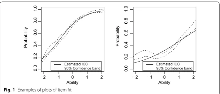
As in Haberman et al. (2013), one can create plots of item fit using the above residuals. Figure 1 shows examples of such plots for two dichotomous items. In each case, p=1 . For each item, the examinee proficiency is plotted along the X-axis, the solid line denotes the values of the estimated ICC, that is, fˆ
j1(1|θ) from Eq. 8 for the item and for the vector θ with the single element θ1, and the two dashed lines denote a pointwise 95 % confidence band consisting of the values of f¯
j1(1|θ)−2sj1(1|θ) and f¯j1(1|θ)+2sj1(1|θ) , where fj¯
1(1|θ) is given by Eq. 7. If the solid line falls outside this confidence band, that would indicate a statistically significant residual. These plots are similar to the plots of item fit provided by IRT software packages such as PARSCALE (Du Toit 2003). In Fig. 1, the right panel corresponds to an item for which substantial misfit is observed and the left panel corresponds to an item for which no statistically significant misfit is observed (the solid line almost always lies within the 95 % confidence band).
(8) tjk(y|θ)=
¯
fjk(y|θ)− ˆfjk(y|θ) sjk(y|θ) ,
i∈Kjk
Wi[ ˆdyijk(θ)]2
ˆ
The ETS mirt software (Haberman 2013) was used to compute residuals for item fit for the NAEP data sets. The program is available on request for noncommercial use.
This item-fit analysis can be considered a more sophisticated version of the graphical item-fit analysis operationally employed in NAEP. While the asymptotic distribution of the residuals is not known in the analysis employed operationally, it is known in our pro-posed item-fit analysis.
Generalized residual analysis
Generalized residual analysis for assessing the fit of IRT models in regular applications (that do not involve complex sampling or matrix sampling) was suggested by Haberman (2009) and Haberman and Sinharay (2013). The methodology is very general and a vari-ety of model-based predictions can be examined under the framework.
For a version of generalized residuals suitable for applications in NAEP, for student i, let Yi be the set of possible values of yi and ei(y,zi) be a real number where zi is the vec-tor of covariates. Let yi∗ be a random variable with values in Yi such that yi∗ and yi are conditionally independent given θi and have the same conditional distribution. Let
let eˆi be the estimated conditional expectation of ei(yi∗,zi) given yi and zi, and let
Let ζˆ and νˆ minimize N
i=1Widˆi2 for
Let s2 be the estimate σˆ2(X¯) for Xi= ˆdi. Then the generalized residual is
Under very general conditions, if the model holds, then t has an asymptotic standard normal distribution (Haberman and Sinharay 2013). A fundamental requirement is that
O=W+−1 N
i=1
Wiei(yi,zi),
ˆ
E=W+−1 N
i=1
Wieˆi(yi,zi).
ˆ
di=ei(yi,zi)− ˆei− ˆζ− ˆν′hiˆ .
t=(O− ˆE)/s.
−2 −1 0 1 2
0.
00
.2
0.
40
.6
0.
81
.0
Ability
Probability
Estimated ICC 95% Confidence band
−2 −1 0 1 2
0.
00
.2
0.
40
.6
0.
81
.0
Ability
Probability
Estimated ICC 95% Confidence band
the dimension q is small relative to N. A normal approximation must be appropriate for ¯
d, where d has values di, 1≤i≤N, such that
minimizes N
i=1E(Widi2).
A statistically significant absolute value of the generalized residual t indicates that the IRT model does not adequately predict the statistic O.
The method is quite flexible. Several common data summaries such as the item pro-portion correct, propro-portion simultaneously correct for a pair of items, and observed score distribution can be expressed as the statistic O by defining ei(yi,zi) appropriately. For example, to study the number-correct score or the first-order marginal distribution of a dichotomous item j related to skill k, let
Then O is the weighted proportion of students who correctly answer item j of subscale k, and t indicates whether O is consistent with the IRT model. Because generalized residu-als for marginal distributions include variability computations based on the IRT model employed, they provide a more rigorous comparison of observed and model-predicted proportions of students obtaining a particular score on an item than provided in Rogers et al. (2006).
For an example of a pairwise number-correct or the second-order marginal distribu-tion, if j and j′ are distinct dichotomous items related to skill k, let
Then O is the weighted proportion of students who correctly answer both item j and item j′, and t indicates whether O is consistent with the IRT model. Residuals for the second-order marginal may be used to detect violations of the conditional independence assumption made by IRT models (Haberman and Sinharay 2013).
It is possible to create graphical plots using these generalized residuals. For example, one can create a plot showing the values of O and a 95 % confidence interval given by
ˆ
E±1.96s. A value of O lying outside this confidence interval would indicate a general-ized residual significant at the 5 % level. The ETS mirt software (Haberman 2013) was used to perform the computations for the generalized residuals.
Assessment of practical significance of misfit of IRT models
George Box commented that all models are wrong (Box and Draper 1987, p. 74). Simi-larly, Lord and Novick (1968, p. 383) wrote that it can be taken for granted that every model is false and that we can prove it so if we collect a sufficiently large sample of data. According to them, the key question, then, is the practical utility of the model, not its ultimate truthfulness. Sinharay and Haberman (2014) therefore recommended the assessment of practical significance of misfit, which comprises the determination of the extent to which the decisions made from the test scores are robust against the misfit of the IRT models. We assess the practical significance of misfit in all of our data examples.
di=ei(yi,zi)−E(ei(yi∗,zi)|yi,zi)−ν′hi(τ)
ei(yi,zi)=
1 ifiis inKjkandyijk =1,
0 otherwise·
ei(yi,zi)=
1 ifiis inKjk∩Kj′kandyijk =yij′k =1,
The quantities of most practical interest among those that are operationally reported in NAEP are the subgroup means and the percent at different proficiency levels. We exam-ine the effect of misfit on these quantities.
Data
We next describe data from four NAEP assessments that are used to demonstrate our suggested residuals. These data sets represent a variety of NAEP assessments.
NAEP 2004 and 2008 long‑term trend mathematics assessment at age 9
The long-term trend Mathematics assessment at age 9 (LTT Math Age 9; see e.g., Rampey et al. 2009) is supposed to measure the students’
• knowledge of basic mathematical facts,
• ability to carry out computations using paper and pencil,
• knowledge of basic measurement formulas as they are applied in geometric setting, and
• ability to apply mathematics to daily-living skills (such as those related to time and money).
The assessment has a computational focus and contained a total of 161 dichotomous multiple-choice and constructed-response items divided over nine booklets. For exam-ple, a multiple-choice question in the assessment, which was answered correctly by 44 % of the examinees, is “How many fifths are equal to one whole?” This assessment has many more items per student than the usual NAEP assessments. The items covered the following topics: numbers and numeration; measurement; shape, size, and position; probability and statistics; and variables and relationships. The data set included about 16,000 examinees most of whom belong to Grade 4 with about 7300 students in the 2004 assessment and about 8600 students in the 2008 assessment. It is assumed in the opera-tional analysis that there is only one skill underlying the items.
NAEP 2002 and 2005 reading at grade 12
NAEP 2007 and 2009 mathematics at grade 8
The NAEP Mathematics Grade 8 assessment measures students’ knowledge and skills in mathematics and students’ ability to apply their knowledge in problem-solving sit-uations. It is assumed that each item measures one among the five following skills (subscales): number properties and operations; measurement; geometry; data analy-sis, statistics and probability; and algebra. This Mathematics Grade 8 assessment (e.g., National Center for Education Statistics 2009) included 231 multiple-choice and con-structed-response items divided over 50 booklets. The full data set included about 314,700 examinees with 153,000 students from the 2007 sample and 161,700 students from the 2009 sample.
NAEP 2009 science at grade 12
The NAEP 2009 Science Grade 12 assessment (e.g., National Center for Education Sta-tistics 2011) included 185 multiple-choice and constructed-response items on physi-cal science, life science, and earth and space science divided over 55 booklets. It is assumed that there is one skill underlying the items. The data set included about 11,100 examinees.
Results for simulated data
In order to check Type I error of the item-fit residuals and the generalized residuals for first-order marginals and second-order marginals, we simulated data that look like the above-mentioned NAEP data sets but fit the model perfectly. The simulations were per-formed on a subset of examinees for Mathematics Grade 8 because of the huge sample size for the test. We used the item-parameter estimates from our analyses of the NAEP data sets using the constrained 3PL/GPCM (see Table 4). Values of θ were drawn from the normal distribution with separate population means for the assessments with two years and unit variance. The original booklet design was used, but sampling weights and primary sampling units were not used.
Item‑fit analysis using residuals Type I error rates
For the item-fit residuals, the average Type I error rates at the 5 % level of signifi-cance over 25 replications, evaluated at either 11 or 31 points, are shown in Table 1. The rates are considerably larger than the nominal level.
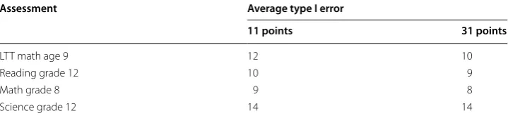
To explore the inflated Type I error rates of the item-fit residuals, Fig. 2 shows the Type I error rates as a function of θ and the test information functions for the four NAEP data sets.
Table 1 Average Type I error for generalized residuals of item response functions Assessment Average type I error
11 points 31 points
LTT math age 9 12 10
Reading grade 12 10 9
Math grade 8 9 8
The item-fit residuals were computed at either 11 or 31 points between −3 and 3. It can be seen that more residuals are significant for larger absolute values of θ, which is in line with earlier results (see, e.g., Haberman et al. 2013; Fig. 2). In addition, there is a relationship between the Type I error rates and the test information function; Type I error rates become larger as information goes down. Obviously, there is a relation-ship between the Type I error rates and the sample sizes. This is best seen for the Sci-ence Grade 12 data set (last row), which is the smallest data set (for which the sample size is about 11,000, with an average of about 1900 responses per item); first, the Type I error rates for item-fit residuals computed at 11 points get closer to the nominal α of .05 than those at 31 points; second, the peak of the test information function is between θ =1 and θ =2, indicating that the items are relatively difficult (note that the mean
−3 −2 −1 0 1 2 3
0.0 0.1 0.2 0.3 0.4 θ
Type I Error
31 points 11 points
−3 −2 −1 0 1 2 3
10 20 30 40 50 θ
−3 −2 −1 0 1 2 3
0.0 0.1 0.2 0.3 0.4 θ
Type I Error
31 points 11 points
−3 −2 −1 0 1 2 3
6 8 10 12 14 16 θ
−3 −2 −1 0 1 2 3
0.0 0.1 0.2 0.3 0.4 θ
Type I Error
31 points 11 points
−3 −2 −1 0 1 2 3
5 10 15 20
θ
−3 −2 −1 0 1 2 3
0.0 0.1 0.2 0.3 0.4 θ
Type I Error
31 points 11 points
−3 −2 −1 0 1 2 3
5 10 15 20 25 θ I ( θ ) I ( θ ) I ( θ ) I ( θ )
and standard deviation of θ are fixed to zero and one for model identification purposes). Given that there are not many students with θ >2 and that even for these students the items can still be relatively difficult, the Type I error rate shows a steep incline between θ =2 and θ =3.
Thus, it can be concluded that the Type I error rates for the item-fit residuals are close to their nominal value if there are enough students and if there is substantial information in the ability range of interest.
Power
The samples of all four NAEP data sets are large and, therefore, the power to detect mis-fit is generally expected to be large; however, we performed additional power analysis for the item fit residuals using the item parameters of the LTT Math Age 9 assessment. Note that this assessment consists of dichotomous items only.
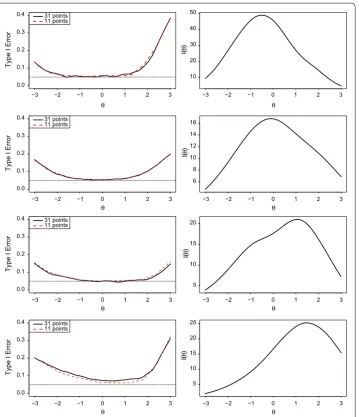
For the item-response functions, we consider four bad/misfitting item types (see e.g., Sinharay 2006, p. 441):
1. Non-monotone for low θ:
p(Y =1|θ )= 14logit−1(−4.25(θ+0.5))+logit−1(4.25(θ−1)).
2. Upper asymptote smaller than 1: p(Y =1|θ )=0.7logit−1(3.4(θ+0.5)).
3. Flat for mid θ: p(Y =1|θ )=0.55logit−1(5.95(θ+1))+logit−1(5.95(θ−2)).
4. Wiggly, non-monotone curve:
p(Y =1|θ )=0.65logit−1(1.5θ )+0.35logit−1(sin(3θ )).
The item response functions for these for item types are shown in Fig. 3. The LTT math age 9 assessments consists of 161 items. We assigned 16 items to be bad items, with each type associated with four items. The simulations are set up in the same way as before, but with the item probabilities for the bad items determined by the equations above.
−3 −2 −1 0 1 2 3
0.0 0.2 0.4 0.6 0.8 1.0
θ
P
Bad item 1: Non−monotone low Bad item 2: Upper assymptote < 1 Bad item 3: Flat middle Bad item 4: Wiggly
The number of replications is 25. The item response functions are again evaluated at 31 points between −3 and 3.
The power for the four bad item types are shown in Table 2. We computed two val-ues of power for each bad item type: one for the 31 points between θ = −3 and θ =3 and one for the 21 points between θ = −2 and θ =2. As expected, both values of power are satisfactory for each bad item type. For bad items of type 4, the values of power are smaller compared to other bad item types, but this is due to the fact that the IRT model can approximate the wiggly curve reasonably well.
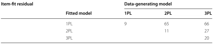
In addition, we simulated data under the 1PL, 2PL, and 3PL model and fitted the 1PL to all three data sets, the 2PL to the latter two, and the 3PL to the latter only. This set up gives us additional Type I error rates for other model types and power for the situation in which the fitted model is simpler than the data-generating model (see e.g., Sinharay
2006; Table 1).
The results of these simulations are shown in Table 3. In this table, the diagonals indi-cate Type I error and the off-diagonals indiindi-cate the power. The Type I Error rates are inflated, which is in line with the previous results. The power to detect misfit of the 1PL is very reasonable, but it is quite low for the 2PL.
Generalized residual analysis
For first-order marginals, or the (weighted) proportion of students who correctly answer the dichotomous items or receive a specific score on a polytomous item, we used 25 rep-lications for each of the four NAEP data sets. For second-order marginals,3 however, we used only five replications, because the computation of these residuals for a single data set is very time consuming (several hours).
For the generalized residuals for first-order marginals, the average Type I error rates at the 5 % level are 7 % for LTT Math Age 9 for long-term trend, 1 % for Reading Grade
3 or the weighted proportion of students who correctly answer a pair of dichotomous items or receive a specific pair of
scores on a pair of items one of which is polytomous.
Table 2 Power of the item-fit residuals for LTT math age 9 simulations
Item type Mean (−3 to 3) Mean (−2 to 2)
Bad item 1 74 84
Bad item 2 96 94
Bad item 3 86 90
Bad item 4 52 68
Table 3 Type I error (diagonals) and Power (off-diagonals) of item-fit residuals for differ-ent model combinations for LTT math age 9
Item‑fit residual Data‑generating model
Fitted model 1PL 2PL 3PL
1PL 9 65 66
2PL 11 27
12, 0 % for Math Grade 8, and 6 % for Science Grade 12, respectively. Note that most of the Type I error rates for the first-order marginals are rather meaningless, because IRT models with item-specific parameters should be able to predict observed item score frequencies well. For the generalized residuals for second-order marginals, the average Type I error rates at the 5 % level are 6 % for LTT Math Age 9, 5 % for Reading Grade 12, and 6 % for Science Grade 12, respectively. Thus, the Type I error rates of the generalized residuals for the second-order marginals are close to the nominal level, and seem to be satisfactory.
Results for the NAEP data
We fitted the 1-parameter logistic (1PL) model, 2PL model, 3PL model with constant guessing (C3PL), and 3PL model to the dichotomous items and the partial credit model (PCM) and GPCM to the polytomous items to each of the above-mentioned data sets. For the LTT Math Age 9, Reading Grade 12, and Math Grade 8 data, which had two assessment years, a dummy predictor was used so that population means for the two years are allowed to differ. The ETS mirt software (Haberman 2013) was used to perform all the computations, including the fitting of the IRT models and the computation of the residuals.
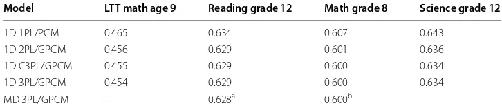
Table 4 shows the estimated expected log penalty per presented item based on the Gilula–Haberman approach. The two missing values in the last row denote that the cor-responding assessments (LTT math and science) involve only one subscale. Note that the multidimensional models are so-called simple structure or between-item multidi-mensional models (e.g., Adams et al. 1997). Before discussing the results, we stress that serious model identification issues were encountered with the 3PL models for all four data sets. First, good starting values needed to be provided in order to find a solution. Second, parameters with very large standard errors were found for the 3PL model. For example, the standard error of the logit of the guessing parameter for one item in the Math Grade 8 data was as high as 20.04, while about 31,200 students answered this item. Note that these issues were not encountered with the C3PL model. Now, we can make two observations based on the results in Table 4. First, there is some improvement in fit when item-specific slope (discrimination) parameters are used: For all four NAEP data sets, the biggest improvement in fit was seen between the unidimensional 1PL/PCM and 2PL/GPCM. Second, the improvement in fit beyond the 2PL/GPCM seems to be small.
Table 4 Relative model fit statistics (PE-GH) for unidimensional (1D) and multidimensional (MD) models
a Three‑dimensional model
b Five‑dimensional model
Model LTT math age 9 Reading grade 12 Math grade 8 Science grade 12
1D 1PL/PCM 0.465 0.634 0.607 0.643
1D 2PL/GPCM 0.456 0.629 0.601 0.636 1D C3PL/GPCM 0.455 0.629 0.600 0.634 1D 3PL/GPCM 0.454 0.629 0.600 0.634
That is, the addition of guessing parameters and multidimensional simple structures only lead to very small improvements in fit.
The estimated correlations between the three (latent) dimensions in the multidimen-sional 3PL/GPCM are .86, .80 and .80 for the Reading assessment. The estimated corre-lations between the five (latent) dimensions in the multidimensional 3PL/GPCM for the Math Grade 8 data are shown in Table 5.
We next summarize the results from the application of our suggested IRT model-fit tools to data from the four above-mentioned NAEP assessments using the unidimen-sional model combinations.
Item‑fit analysis using residuals
For each of the four NAEP data sets, we computed the item-fit residuals at 31 equally-spaced values of the proficiency scale between −3 and 3 for each score category (except for the lowest score category) of each item. Haberman et al. (2013) recommended the use of 31 values. Further, some limited analysis showed that the use of a different num-ber of values does not change the conclusions. This resulted in, for example, 31 residuals for a binary item and 62 residuals for a polytomous item with three score categories.
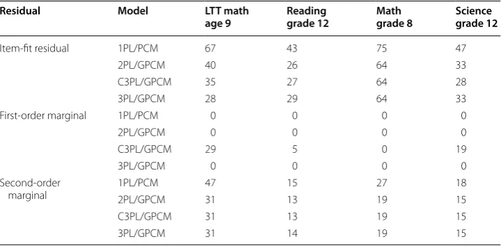
The results are shown in Table 6. The percentages of significant results for the item-fit residuals are all much larger than the nominal level of 5 %. There is a substantial drop in the percentages from the 1PL/PCM to the other three models. However, the percentages show a steady decrease only for the LTT Math Age 9 assessments with increasing model
Table 5 Correlations between dimensions in five-dimensional 3PL/GPCM for math grade 8 data
2 3 4 5
1. Number properties and operations .97 .93 .96 .95
2. Measurement – .96 .96 .94
3. Geometry – .93 .92
4. Data analysis and probability – .94
5. Algebra –
Table 6 Percent significant residuals under different unidimensional models Residual Model LTT math
age 9 Reading grade 12 Math grade 8 Science grade 12
Item-fit residual 1PL/PCM 67 43 75 47
2PL/GPCM 40 26 64 33
C3PL/GPCM 35 27 64 28
3PL/GPCM 28 29 64 33
First-order marginal 1PL/PCM 0 0 0 0
2PL/GPCM 0 0 0 0
C3PL/GPCM 29 5 0 19
3PL/GPCM 0 0 0 0
Second-order
marginal 1PL/PCM2PL/GPCM 4731 1513 2719 1815
C3PL/GPCM 31 13 19 15
complexity (note that this assessment contains the largest proportion of MC items). For the other three data sets, the percentages of significant residuals are similar after the 2PL/GPCM.
In the operational analysis, the number of items that were found to be misfitting and removed from the final computations were two, one, zero and six, respectively, for the four assessments.
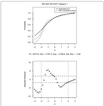
Figure 4 shows the item-fit plots and residuals for a constructed response item from the 2005 Reading Grade 12 assessment. In the top panel, the solid line shows the esti-mated ICC of the item (fˆ
j1(1|θ) from Eq. 8) and the dashed lines show a corresponding pointwise 95 % confidence band (f¯
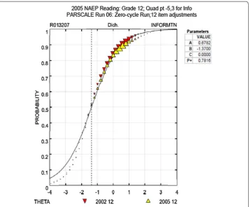
j1(1|θ)−2sj1(1|θ) and f¯j1(1|θ)+2sj1(1|θ)). The bot-tom panel shows the residuals. The figure shows that several residuals are statistically significant. In fact, except for three or four residuals, all the residuals are statistically significant. In addition, several of them are larger than 5. Thus, the 2PL model does not fit the item. Figure 5 shows the operational item fit plot (PARPLOT) for the same item. The plot shows the estimated ICC using a solid line. The triangles indicate the “empir-ical ICC” and the inverted triangles indicate the “empir“empir-ical ICC” during the previous
−3 −2 −1 0 1 2 3
0.0 0.2 0.4 0.6 0.8 1.0
050 Item R013207 Category 1
N = 3475.9; Obs. = 2797.3; Exp. = 2796.6; Adj. Res. = 0.00
θ
Probability
Estimated ICC 95% Confidence band
−3 −2 −1 0 1 2 3
−10 −5 0 5 10
θ
Adjusted Residual
administration of the same item (in 2004). In NAEP operational analysis, the misfit of the item was not found serious—so the item was retained.
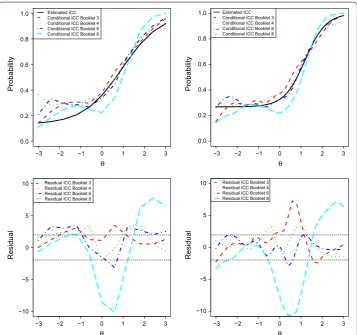
The item fit residuals can also be used to check if the item response function of a par-ticular item provides sufficient fit across all different booklets that contain the item. This provides an opportunity to study item misfit due to, for example, item position effects (e.g., items that are at the end of the booklet can be more difficult due to either speeded-ness or fatigue effects; see, for example, Debeer and Janssen 2013). Figure 6 shows the item fit residuals per booklet for a multiple choice LTT Math Age 9 item. It can be seen that the fit residuals for lower abilities improve if the 3PL is used instead of the 3PL. Interestingly, the residuals for booklet 8 are more extreme than those for the other three booklets.
Generalized residual analysis
The second block of Table 6 shows the percentage of statistically significant generalized residuals for the first-order marginal without any adjustment (that is, larger than 1.96 in absolute value) for all data sets and different models. The percentages are all zero except for the C3PL/GPCM. This can be explained by the fact that all but the C3PL/GPCM have item-specific parameters that can predict the observed proportions of item scores quite well. Only the C3PL/GPCM can have issues with this prediction, for example, if there is variation in guessing behaviors. This latter seems to be the case for LTT Math Age 9 but not for Math Grade 8.
The third block of Table 6 shows the percentage of statistically significant generalized residuals for the second-order marginals. The percentages are considerably larger than the nominal level (also than the Type I error rates found in the simulation study) and show that the NAEP model does not adequately account for the association among the items. The misfit is most apparent for LTT math age 9.
Figure 7 shows a histogram of the generalized residuals for the second order marginal for the 2009 Science Grade 12 data.
Several generalized residuals are smaller than −10, which provides strong evidence of misfit of the IRT model to second-order marginals.
Researcher such as Bradlow et al. (1999) noted that if the IRT model cannot account for the dependence between item-pair properly, then the precision of proficiency esti-mates will be overestimated and showed that accounting for the dependence using, for example, the testlet model would not lead to overestimation of the precision of pro-ficiency estimates. Their result implies that if we found too many significant general-ized residuals for second-order marginals for items belonging to common stimulus (also referred to as testlets by, for example, Bradlow et al. 1999), then application of a model like the testlet model (Bradlow et al. 1999) would lead to better fit to the NAEP data. However, we found that the proportion of significant generalized residuals for
−3 −2 −1 0 1 2 3
0.0 0.2 0.4 0.6 0.8 1.0 θ Probabilit y Estimated ICC Conditional ICC Booklet 3 Conditional ICC Booklet 4 Conditional ICC Booklet 6 Conditional ICC Booklet 8
−3 −2 −1 0 1 2 3
−10 −5 0 5 10 θ Residual
Residual ICC Booklet 3 Residual ICC Booklet 4 Residual ICC Booklet 6 Residual ICC Booklet 8
−3 −2 −1 0 1 2 3
0.0 0.2 0.4 0.6 0.8 1.0 θ Probabilit y Estimated ICC Conditional ICC Booklet 3 Conditional ICC Booklet 4 Conditional ICC Booklet 6 Conditional ICC Booklet 8
−3 −2 −1 0 1 2 3
−10 −5 0 5 10 θ Residual
Residual ICC Booklet 3 Residual ICC Booklet 4 Residual ICC Booklet 6 Residual ICC Booklet 8
second-order marginals for item pairs belonging to testlets is roughly the same as those for item pairs not belonging to testlets. Thus, there does not seem to be an easy way to rectify the misfit of the NAEP IRT model to the second-order marginals.
Assessment of practical significance of misfit
To assess the practical significance of item misfit for the four assessments, we obtained the overall and subgroup means and the percentage of examinees at different proficiency levels (we considered the percentages at basic or above, and proficient or above) from the operational analysis. These quantities are reported as rounded integers in operational NAEP reports (e.g., Rampey et al. 2009). Note that these quantities were computed after omitting the items that were found misfitting in the operational analysis (2, 1, 0 and 6 such items for the four assessments). Then, for any assessment, we found the nine items that had the largest number of statistically significant item-fit residuals. For example, for the 2008 long-term trend Mathematics assessment at Age 9, nine items with respectively 19, 19, 19, 19, 18, 18, 17, 17 and 16 statistically significant item-fit residuals (out of a total of 31 each) were found.
For each assessment, we omitted scores on the nine misfitting items and ran the NAEP operational analysis to recompute the subgroup means (rounded and converted to the NAEP operational score scale) and the percentage of examinees at different proficiency levels. We compared these recomputed values to the corresponding original (and opera-tionally reported) quantities.
Interestingly, in 48 such comparisons of means and percentages for each of the four data sets, there was no difference in 44, 36, 32 and 47 cases, respectively, for the long-term-trend, reading, math and science data sets. For example, the overall average score is 243 (on a 0-500 scale) and overall percent scoring 200 or above is 89 in both of these analyses for the 2008 long-term-trend Mathematics assessment at age 9. In the cases when there was a difference, the difference was one in absolute value. For example, the
Generalized residuals
Relativ
e frequenc
y
−40 −30 −20 −10 0 10 20 30
0.00
0.05
0.10
0.15
0.20
0.25
0.30
0.35
operationally reported overall percent at 250 or above is 44 while the percent at 250 or above after removing 9 misfitting items is 45 for the 2008 long-term-trend Mathematics assessment at age 9.
Thus, the practical significance of the item misfit seems to be negligible for the four data sets.
Conclusions
The focus of this paper was on the assessment of misfit of the IRT model used in large-scale survey assessments such as NAEP using data from four NAEP assessments. Two sets of recently suggested model-fit tools, the item-fit residuals (Bock and Haberman
2009; Haberman et al. 2013) and generalized residuals (Haberman and Sinharay 2013), were modified for application to NAEP data.
Keeping in mind the importance of NAEP in educational policy-making in the U.S., this paper promises to make a significant contribution by performing a rigorous check of the fit of the NAEP model. Replacement of the current NAEP item-fit procedure by our suggested procedure would make the NAEP statistical toolkit more rigorous. Because several other assessments such as IALS, TIMSS and PIRLS use essentially the same sta-tistical model as in NAEP, the findings of this paper will be relevant to those assessments as well.
An important finding in this paper is that statistically significant misfit (in the form of significant residuals) was found for all the data sets. This finding concurs with the state-ment of George Box that all models are wrong (Box and Draper 1987, p. 74) and a simi-lar statement of (Lord and Novick 1968, p. 383). However, the observed misfit was not practically significant for any of the data sets. For example, the item-fit residuals were statistically significant for several items, but the removal of some of these items led to negligible differences in the reported outcomes such as subgroup means and percentages at different proficiency levels. Therefore, the NAEP operational model seems to be use-ful though it is “wrong” (in the sense that the model was found misfitting to the NAEP data using the suggested residuals) from the viewpoint of George Box. It is possible that the lack of practical significance of the misfit is due to the thorough test development and review procedures used in NAEP, which may filter out any serious IRT-model-fit issues. The finding of the lack of practical significance of the misfit is similar to the find-ing in Sinharay and Haberman (2014) that the misfit of the operational IRT model used in several large-scale high-stakes tests is not significant.
DIF and multidimensionality (e.g., Camilli 1992) and it would be of interest to study the practical consequences of multidimensionality on DIF. Fourth, it is possible to further explore the reasons of the first-order marginal not being useful in our analysis. Sinharay et al. (2011) also found the generalized residuals of Haberman and Sinharay (2013) for the first-order marginal to be not useful in assessing the fit of regular IRT models. These residuals might be more useful to detect differential item functioning (DIF). For exam-ple, the generalized residuals for the first-order marginals for males and females can be used to study gender-based DIF (although the Type I error might be low, the power would be larger). Finally, several students taking the NAEP, especially those in twelfth grade, lack motivation (e.g., Pellegrino et al. 1999). It would be interesting to examine whether that lack of motivation affects the model fit in any manner.
Authors’ contributions
PWVR carried out most of the computations and wrote a major part of the manuscript. SS wrote the first draft of the manuscript and performed some of the computations. SJH suggested the mathematical results. MSJ wrote some parts of the manuscript and performed some computations. All authors read and approved the final manuscript.
Author details
1 ETS Global, Amsterdam, Netherlands. 2 Pacific Metrics Corporation, Monterey, CA, USA . 3 ETS, Princeton, NJ, USA. 4 Columbia University, New York, USA.
Acknowledgements
The authors thank the editor Matthias von Davier and the two anonymous reviewers for helpful comments. The research reported here was partially supported by the Institute of Education Sciences, U.S. Department of Education, through Grant R305D120006 to Educational Testing Service as part of the Statistical and Research Methodology in Education Initiative.
Competing interests
The authors declare that they have no competing interests.
Received: 24 September 2015 Accepted: 7 June 2016
References
Adams, R. J., Wilson, M. R., & Wang, W. C. (1997). The multidimensional random coefficients multinomial logit model.
Applied Psychological Measurement, 21, 1–23.
Allen, N. A., Donoghue, J. R., & Schoeps, T. L. (2001). The NAEP 1998 technical report (NCES 2001-452). Washington, DC: United States Department of Education, Institute of Education Sciences, Department of Education, Office for Educa-tional Research and Improvement.
American Association of Educational Research, American Psychological Association, & National Council on Measurement in Education. (2014). Standards for educational and psychological testing. Washington, DC: American Educational Research Association.
Beaton, A. E. (1987). Implementing the new design: The NAEP 1983–84 technical report (Tech. Rep. No 15-TR-20). Prince-ton, NJ: ETS.
Beaton, A. E. (2003). A procedure for testing the fit of IRT models for special populations: Draft. Unpublished manuscript. Birnbaum, A. (1968). Some latent trait models and their use in inferring an examinee’s ability. In F. M. Lord & M. R. Novick
(Eds.), Statistical theories of mental test scores (pp. 397–479). Reading: Addison-Wesley.
Bock, R. D., & Haberman, S. J. (2009) Confidence bands for examining goodness-of-fit of estimated item response func-tions. Paper presented at the annual meeting of the Psychometric Society, Cambridge, UK.
Box, G. E. P., & Draper, N. R. (1987). Empirical model-building and response surfaces. New York, NY: Wiley.
Bradlow, E. T., Wainer, H., & Wang, X. (1999). A Bayesian random effects model for testlets. Psychometrika, 64, 153–168. Camilli, G. (1992). A conceptual analysis of differential item functioning in terms of a multidimensional item response
model. Applied Psychological Measurement, 16, 129–147. Cochran, W. G. (1977). Sampling techniques (3rd ed.). New York: Wiley.
Debeer, D., & Janssen, R. (2013). Modeling item-position effects within an IRT framework. Journal of Educational Measure-ment, 50, 164–185.
Dresher, A. R., & Thind, S. K. (2007). Examination of item fit for individual jurisdictions in NAEP. Paper presented at the annual meeting of the American Educational Research Association, Chicago, IL.
du Toit, M. (2003). IRT from SSI. Lincolnwood, IL: Scientific Software International.
Efron, B., & Tibshirani, R. J. (1993). An introduction to the bootstrap. New York: Chapman and Hall.
Gilula, Z., & Haberman, S. J. (1995). Prediction functions for categorical panel data. The Annals of Statistics, 23, 1130–1142. Gilula, Z., & Haberman, S. J. (1994). Models for analyzing categorical panel data. Journal of the American Statistical
Haberman, S. J. (2009). Use of generalized residuals to examine goodness of fit of item response models (ETS Research Report RR-09-15). Princeton: ETS.
Haberman, S. J. (2013). A general program for item-response analysis that employs the stabilized Newton-Raphson algorithm (ETS Research Report RR-13-32). Princeton: ETS.
Haberman, S. J., & Sinharay, S. (2013). Generalized residuals for general models for contingency tables with application to item response theory. Journal of American Statistical Association, 108, 1435–1444.
Haberman, S. J., Sinharay, S., & Chon, K. H. (2013). Assessing item fit for unidimensional item response theory models using residuals from estimated item response functions. Psychometrika, 78, 417–440.
Kirsch, I. S. (2001). The International Adult Literacy Survey (IALS): Understanding what was measured (ETS Research Report RR-01-25). Princeton: ETS.
Li, J. (2005) The effect of accommodations for students with disabilities: An item fit analysis. Paper presented at the Annual meeting of the National Council of Measurement in Education, Montreal, CA.
Lord, F. M., & Novick, M. R. (1968). Statistical theories of mental test scores. Reading: Addison Wesley.
Martin, M. O., & Kelly, D. L. (1996). Third international mathematics and science study technical report volume 1: Design and development. Chestnut Hill: Boston College.
Mislevy, R. J., Johnson, E. G., & Muraki, E. (1992). Scaling procedures in NAEP. Journal of Educational Statistics, 17, 131–154. Mullis, I., Martin, M., & Gonzalez, E. (2003). 2003 PIRLS 2001 international report: IEA’s study of reading literacy achievement in
primary schools,. Chestnut Hill: Boston College.
Muraki, E. (1992). A generalized partial credit model: Application of an EM algorithm. Applied Psychological Measurement,
16, 159–176.
National Center for Education Statistics. (2009). The nations report card: Mathematics 2009 (Tech. Rep. No. NCES 2010451). Washington, DC: Institute of Education Sciences, U.S. Department of Education.
National Center for Education Statistics. (2011). The nations report card: Science 2009 (Tech. Rep. No. NCES 2011451). Wash-ington, DC: Institute of Education Sciences, U.S. Department of Education.
Orlando, M., & Thissen, D. (2000). Likelihood-based item-fit indices for dichotomous item response theory models. Applied Psychological Measurement, 24, 50–64.
Pellegrino, J. W., Jones, L. R., & Mitchell, K. J. (1999). Grading the nation’s report card: Evaluating NAEP and transforming the assessment of educational progress. Washington, DC: National Academy Press.
Perie, M., Grigg, W., & Donahue, P. (2005). The nation’s report card: Reading 2005 (Tech. Rep. No. NCES 2006451). Washing-ton, DC: U.S. Government Printing Office: U.S. Department of Education, National Center for Education Statistics. Rampey, B. D., Dion, G. S., & Donahue, P. L. (2009). NAEP 2008 trends in academic progress (Tech. Rep. No. NCES 2009479).
Washington, DC: National Center for Education Statistics, Institute of Education Sciences, U.S. Department of Education.
Rogers, A., Gregory, K., Davis, S., Kulick, E. (2006). Users guide to NAEP model-based p-value programs. Unpublished manuscript. Princeton: ETS.
Sinharay, S. (2006). Bayesian item fit analysis for unidimensional item response theory models. British Journal of Math-ematical and Statistical Psychology, 59, 429–449.
Sinharay, S., Guo, Z., von Davier, M., & Veldkamp, B. P. (2010). Assessing fit of latent regression models. IERI Monograph Series, 3, 35–55.
Sinharay, S., & Haberman, S. J. (2014). How often is the misfit of item response theory models practically significant?
Educational Measurement: Issues and practice, 33(1), 23–35.
Sinharay, S., Haberman, S. J., & Jia, H. (2011). Fit of item response theory models: A survey of data from several operational tests (ETS Research Report No. RR-11-29). Princeton: ETS.