On Expressive Construction of Solitons from Physiological Wave Phenomena

Published online July 20, 2014 (http://www.sciencepublishinggroup.com/j/pamj) doi: 10.11648/j.pamj.20140303.13

ISSN: 2326-9790 (Print); ISSN: 2326-9812 (Online)

On expressive construction of solitons from

physiological wave phenomena

Nzerem Francis Egenti

Department of Mathematics & Statistics, University of Port Harcourt, Nigeria

Email address:

[email protected]

To cite this article:

Nzerem Francis Egenti. On Expressive Construction of Solitons from Physiological Wave Phenomena. Pure and Applied Mathematics Journal. Vol. 3, No. 3, 2014, pp. 70-77. doi: 10.11648/j.pamj.20140303.13

Abstract:

Physiological waves, much like the waves of some other physical phenomena, consist of non-linear and dispersive terms. In studies involving patho-physiology, models on arterial pulse waves indicate that the waveforms behave like solitons. The Korteweg-deVrie (KdV) equation, which is known to admit soliton solutions, is seen to hold well for arterial pulse waves. The foregoing underpins the need for detailed knowledge of the construction of solitons. In the light of this, plane wave solution would fail to yield the desired goal, let alone wherearterial pulse waves are physiological waves that decompose into a travelling wave representing fast transmission phenomena during systolic phase and a windkessel term representing slow transmission phenomena during diastolic phase. This paper elucidates the construction of the solitons that arise from the so called KdV equation. The goal is to enhance an authentic analysis of soliton-based clinical details.

Keywords:

Mathematical, Bilinear, Asymptotic Expansion, Pulse Wave, Systolic and Diastolic

1. Introduction

A major issue that physical problems contend with is the form in which a partial differential equation (PDE) appears. In many cases we suffer the sight of hideous PDEs that arise from physical problems. Such PDEs appear in some form that defies mathematical analysis. Lamentably, understandable solution is imperative if physiological exigencies must have mathematical analysis. We should note that solutions may not be approximated by plane wave solution in physiological cases; they may require exponentially decaying solutions. Many conditions that do not apply to physiological phenomena may hold well for other similar physical phenomena. To this end, it would be customary to talk of physiological wave to stress the divorce between such wave and a group of other physical waves. In general, two major wave phenomena are the

peaking and steepening morphologies. Solitons are isolated waves that travel without dissipating energy. They are a product of wave phenomena. Many studies on waves show that physiological waves are known to behave like solitons (rather than sinusoid). Arterial pulse waves are physiological waves that decompose into a travelling wave representing fast transmission phenomena during systolic

phase and a windkessel term representing slow transmission phenomena during diastolic phase [1]. Solitons are evident at the systolic phase, and the diastolic phase is marked by slow flow waves. In this regard, it was indicated [2] that soliton-based signal processing, together with a windkessel model may be used to compute blood pressure wave in large proximal arteries. By simple theories, linear waves are subject to superposition. Interestingly, non-linear waves are amenable to superposition [3]. The suitability of constructing soliton solutions derives from linear superposition of non-linear waveform so obtained from any given problem.

only two solitons may be enough to describe the peaking and steepening wave phenomena. The question of how linear superposition of non-linear waves can be achieved is answered by careful construction of solitons. Although the

inverse scattering method of solution of some PDEs due to Gardner et al. [9, 10] may bring to bear on solution of the KdV equation, two methods of such construction shall be discussed in this paper. One of the methods, due to Malfliet [11, 12], is the hyperbolic tangent (tanh) method. The other method, due to Hirota [13], is the bilinear method.Each of these methods has its peculiar way of furnishing solitons. We do not lose cognizance of the existence of some other methods of solution of the KdV equation. A particular case is the homotopy analysis method [14, 15]. The analysis of physiological waves relies abundantly on solitons. Much as two solitons can describe any patho-physiological content of a human subject (as shown by Nzerem and Alozie [6], Nzerem and Ugorji [7]), it would be more rewarding to observe the behavior of more solitons in the pressure wave spectrum of the cardio-vascular system. This line of thought gives credo to the bilinear method, due to its propensity to furnish as many solitons as necessary, albeit with expensive algebra.

2. Constructing Solitons via Methods of

Solution

2.1. The Tanh (Hyperbolic Tangent) Method of Solution

In the previous section we have said that KdV equation describes physiological waves. In this section we shall use two methods to construct soliton solution of the KdV equation. The KdV equation is given by

ut+ auux+ buxxx = 0 (2.1)

where a and b (> 0) are parameters. Equation (2.1) shows the dependence of the rate of change of the wave’s height in time on the sum of the nonlinear term (the amplitude effect), and the dispersive term (that causes waves of different wavelengths to propagate at different velocities). Our task in this sub-section is to construct one soliton solution (1SS)of the equation (2.1).

In equation (2.1), the parameter b represents a dispersive effect. A brief description of the tanh method is given below [16] .Suppose

ut = G(u, ux, uxx, …) . (2.2)

Does equation (2.1) admits exact traveling wave solution?

If yes, then we wish to compute it. In the first place, the independent variables t and x are combined into a new variable, ξ = k(x – Vt), which defines the traveling frame of reference, k > 0 being the wave number and V the velocity of wave. In most cases ODEs are more tractable than PDEs. This method seeks a reduction of PDEs to ODEs so that solutions may be easier. By replacing the variable u(x, t)

by U(ξ),equation (2. 1) is transformed into

...) , 2 2 2 , , (

ξ ξ

ξ _d

U d k d dU k U G d dU

kV =

− . (2.3)

We observe that equation (2.3) is an ODE instead of a PDE. We then seek exact solution of the ODEs in tanh form; otherwise an approximate solution may be sought. Introduce a new variable Y = tanh ξ into the ODE. Now the coefficient of the ODE in U(ξ) = F(Y) solely depends on Y

because

ξ

d d

and subsequent derivatives in (2.3) are

replaced by

( )

dY d Y2

1− .

We seek solution as finite power series in Y in the form

n n N

0 n

Y a ) Y (

F

∑

=

= . (2.4)

The equation (2.1) transforms into

0 d

U d bk d dU U d dU

kV ₃

3

3 ₌

ξ + ξ + ξ

− . (2.5)

Introduce Y = tanh(ξ) and thus replace equation (2.5) by

dY Y dF Y Y kF dY

Y dF Y

kV(1− 2) ( )+ ( )(1− 2) ( )

−

0 ) ( ) 1 ( ) 1 ( ) 1

( 2 2 2

3 ₌

  

  

   

 

− −

− +

dY Y dF Y dY

d Y dY

d Y

bk (2.6)

From equation (2.4) we get

2

0 1

0

) 1 ( )

( ,

)

( ₋

= −

=

− =

     

=

∑

∑

n

n N

n n

n N

n

Y a n n dY

Y dF dY

d Y na dY

Y dF

Substitute the above equations into equation (2.6) (with the range of summation assumed known) to get

[

+1₋ −1

] [

₋ 2 2 +1₋ 2 2n−1

]

n n

n n

n n

nY ΣnaY kΣΣna Y ΣΣna Y

na Σ kV

[

3 2 1 2 1

]

3

) 2 2

( )

2 3 3 ( )

1

( − − − − + − + + + +

+ n

n n

n n

nY Σn n n aY Σn n n aY

a n n Σ bk

0 )

2

( + 3 =

− n+

nY a n n

Σ (2.7)

We note a salient aspect of this method: the terms of the series must terminate, and thus we do not expect recurrent

equate the highest two powers of n = N to get 2N + 1 = N + 3 i.e. N = 2. With this, equation (2.4) reads

F(Y) = a0 + a1Y +a2Y2 (2.8)

Substitute (2.8) into (2.6), noting that

Y a a Y F dY

Y dF

2 1 2 ) ( ' ) (

+ =

= .

With this we get

– kV[(1 – Y2)(a1 + 2a2Y)] + k[(a0 + a1Y + a2Y2)(1 – Y2)(a1

+ 2a2Y)]

+ bk3_{[(1 – Y}2_)(–2a

1 – 16a2Y + 6a1Y2 + 24a2Y3)]=0.

The expanded form yields

– kV(a1 + 2a2Y – a1Y2 – 2a2Y3) +

2 1 0 2 1 2

0 2 1 1

0 ( 2 ) (3 )

[(aa a aa Y aa aa Y

k + + + −

] 2 3

) 2 2

( a₂2−a₁2− a₀a₂ Y3− a₁a₂Y4− a2₂Y5

+

[

2₁ 16 ₂ 8₁ 2 40 ₂ 3 6 ₁ 4 24 ₂ 5

]

0

3_{− − + + − − =}

+bk a aY aY aY aY aY (2.9)

For the series to vanish, the coefficients of the powers of

Y must vanish identically. Thus, we equate the coefficient of each of the powers of Y to zero.

In doing so we find that the coefficients that are enough to yield a desired result are those of Y2and Y5, which read respectively,

a1k[V + 3a2 – a0 + 8bk2] = 0 (2.10)

–2a2k[a2 + 12bk2] = 0 (2.11)

If a1=a2=0 we get, in equation (2.10), V = a0-8bk. It is permissible to use a2 = –12bk2 in(2.11). Thus, for a1= 0 we

have, using (2.8)

F(Y) = a0 – 12bk2Y2 (2.12)

Suppose the solution vanishes for ξ→∞(Y → 1), we get

F(Y) = 12bk2 (1 – Y2) with V = 4bk2 (2.13)

Or, using the original variables, we get the 1SS

u(x, t) = 12bk2 _sech2_{k(x – Vt). (2.14)}

This is a solitary wave in a bell-shape, as shown in Figure 2.1. A variety of methods, such as, tanh-sech

method, extended tanh method, hyperbolic function method, etc. may be engaged in finding an exact solitary wave solution of nonlinear PDEs. The main issue is the relative ease with which multi-solitons can be generated from ISS.

2.2. Bilinear Method

The bilinear method [13] provides an elegant direct technique for constructing exact solutions to many non-linear PDEs. If one is only interested in finding multi-soliton solutions the best tool is the bilinear method [17, 18]. So long as the bilinear form is obtained, an algorithmic procedure follows. The method relies on calculus and algebra. In application, the bilinear method requires [19]:

(i) A change of dependent variable;

(ii) Introduction of a novel differential operator; (iii) A perturbation expansion to solve the emerging bilinear equation.

Dependent variables are in their best forms when soliton solutions appear as a finite sum of exponentials. Let a variable u be given by

M

u=2∂2xlogdet (2.15)

where the entries of M are polynomials of exponentials

eax+bt. We want to obtain a form that would facilitate the construction of soliton solutions. Defined a new dependent variable by

f

u=2∂2xlog (2.16)

Suppose f(x) and g(x) is some ordered pair of functions. We write the Hirota differential operator Dx defined on the

f(x) and g(x) as

Dx (f⋅g) =

(

∂x1−∂x2

)

f x g x x1=x2=x

) ( )

( _{1 2 (2.17)}

In general

t t t

x x x n

t t m x x n

t m

xD f g f x t g x t

D

= =

= =

∂ − ∂ ∂ − ∂ = ⋅

2 1

2 1 2

1 2

1 ) ( ) ( , ) ( , )

( )

( _{1 1 2 2 , (2.18)}

where m and n are non-negative integers. There is linearity in both arguments of the differential operator, and thus it is called a bilinear operator. The bilinear operators in equations (2.17)and (2.18) have the following properties:

m m m

x

x f f

D

∂ ∂ = ⋅1)

( (2.19)

) ( ) 1 ( )

(f g D g f

D_xm ⋅ = − m _xm ⋅ (2.20)

0 ) (f⋅f =

Dm_x , for m odd (2.21)

t x k k n m

t x k t x k n t m

xD e e k k e

Let P(Dx, Dt) be a polynomial in Dx and Dt. Then, from (2.19) and (2.22) we progress as follows: Let

= ⋅ −

− ₎

(_ek1x ω1t _ek2x ω2t

(

_e(k1+k2)−(ω1+ω2)t⋅₁

)

_(2.23)

From (2.22) we have

(

1

)

) ,

( (k1+k2)−( 1+ 2)t⋅ t

x D e

D

P ω ω ≡P₍D_x,D_t)

( ) (

f_.1 Pk k _,

) (

P D_x,D_t

)

e(k1 k2) (x 1 2)t 2

1 2

1+ −

ω

−

ω

+ −ω+ω

=

We, therefore have the result,

(

1

)

) , ( ) ,

(

) ,

( ) )(

( ( ) ( )

2 1 2 1

2 1 2

1 1 2 1 2

2 2 1

1 ⋅

− − +

+ − − =

⋅ − + − +

− k k t

t x t

x k t x k t

x P D D e

k k P

k k P e

e D D

P ω ω ω ω

ω ω

ω ω

(2.24)

Consider once more, the KdV equation (2.1)in the form

uxxx + 6uux + ut = 0 (2.25)

The present aim is to make it amenable to the bilinear method. We seek a bilinear form. To do this we carry out the dependent variable transformation

    

 

 ₋

= ∂

∂

=2 2₂ log 2 ₂ 2

f f ff f x

u xx x

(2.26)

With this, equation (2.25) becomes

2(logf)xxt + 3∂x(u2) + u3x = 0 (2.27)

Integrating once with respect to x to get

2(logf)xt + 3u2 + u2x = 0 (2.28)

We therefore calculate the relevant quantities as follows:

3 2 2 4

2 _{4 4 8}

f f f f

f f

f

u x xx_ − x xx

    

+

     

= (2.29)

f f

f f f f f

f f f f

f

u x x x x x x₂3x 4x

2 2 3

2 2 4

2 12 24 6  −8 +2

    

−

       

+

     

−

= (2.30)

    

  

− −

=

f f f

f f

f x t xt

xt 2 ₂

) (log

2 (2.31)

Substitute (2.29) - (2.31) in (2.28), and perform the necessary algebra, to get

ffxt – fxft + ff4x – 4fxf3x +

3

0

2 2x

=

f

(2.32)

The above (2.32) is a quadratic equation in f2x. Define Hirota D-operator by

x x x m

m

x f g x x f x g x

D ⋅ = ∂ −∂ _{= =}

2 1

) ( ) ( )

( _{1 2 1 2 (2.33)}

Consider the two relations

DxDt f⋅f = 2(ftx f – ft fx) (2.34)

) 3 4

(

2 _{4 3 2}2

4

x x x x

xf f ff f f f

D ⋅ = − + (2.35)

Add (2.34) to (2.35) to get the bilinear form

) ( )

(D D3 f f B f f

Dx t + x ⋅ ≡ ⋅ = 0; (see equation (2.32)) (2.36)

where B abbreviates the bilinear operator for the KdV equation. The above bilinear equation therefore holds well for the KdV equation.

2.3. Solitons by Bilinear Method

The bilinear form (2.36) enables us to construct soliton solutions for the KdV equation. Consider a class of bilinear equations of the form

P (Dx, Dt, …) f⋅f ≝ Dx(Dt+Dx3)f⋅f =0≡B(f ⋅f) (2.37) where P is a polynomial in the Hirota partial derivatives D. We start with the zero-soliton solution ((OSS) or the vacuum).The KdV equation has a trivial solution u ≡ 0. We therefore require the corresponding f. From equation (2.16) we see that f =e2∝ (t) x + (t) _{is suitable for equation (2.2 6).}

We are free to choose f = 1 as an OSS. It solves equation (2.37) so long as

P (0, 0, …) = 0. (2.38)

Multi-soliton solutions can be obtained by finite perturbation expansions around the vacuum f = 1. To do this, seek a series solution of the form

n n N

n f

f

∑

υ

=

+ =

1

1 , (2.39)

for some unknown functions f1(x,t), f2(x,t),.., where

υ

is a formal expansion parameter. Substituting (2. 39) into (2.36) and equating to zero the powers of

υ

yield

O(

υ

0_{) : B(1⋅1) = 0 (2.40)}

O(

υ

1) : B(1⋅f1 + f1⋅1) = 0 (2.41)

O(

υ

2) : B(1⋅f2 + f1⋅f1 + f2⋅1) = 0 (2.42)

O(

υ

3) : B(1⋅f3 + f1⋅f2 + f2⋅f1 + f3⋅1) = 0

0 : ) ( 0 =         ⋅ − =

∑

j n j

n j n f f B

O

υ

, with f0 = 1 (2.44)

For the KdV equation, the operator B is defined in (2.36). Since the KdV equation admits N–solition solutions [20] equation (2.39) will terminate at n = N<∞ (this is an essential feature of Hirota method – a case where there exists a finite number of terms of the series), provided f1 is the sum of precisely N simple exponential terms. We obtain ISS (N = 1) from

f1 = expθ = exp (kx – ωt + δ),

where k, ω and δ are constants. The dispersion law

ω = k3 _(2.45)

is determined by (2.41). Equation (2.42) permits us to set f2

= 0, and in effect we can take fi = 0 for i > 2. Let υ= 1, and we get

f = 1 + f1 = 1 + expθ = 1 + exp(kx – ω+ δ).

Substitute f in (2.28) with (2.45), and get

        ₋ = ∂ ∂

= 2 ₂ 2

2 2 2 ) , ( log 2 ) , ( f f ff x t x f t x

u x x

For a 1SS we write

( ) ( ( ))

₍

₎

_{( ( )}( )₎2 2 2 2 2 2 exp 1 exp 2 1 2 exp 1 log 2 , ζ ζ δ ω δ ω δ ω + = + = ∂ + − + ∂ = + − + − _k e e k x t kx t x u t kx t kx (2.46)

where ζ =kx−ωt+δ . The last expression of equations (2.46) takes the form of Padéapproximant (Curry (2008)), which describes the function

( )

      = 2 sec 2 , 2 2 _ζ h k t x u

Substitute ζ =kx−ωt+δand get

u(x,t) ( )

2 1 sec 2

1 2 2 ₋ 3 _+δ

= k h kx k t

Let k = 2K; we get

u(x, t) = 2K2_sech2_{(Kx – 4K}3_{t + δ/2) . (2.47)} The above is a pulse shaped solitary wave solution of the KdV equation, and it compares to the solution (2.14) (see Fig 2.1).

The construction of the 2SS can help in producing N (>2) solutions. Consider the 1SS (2.47) and, for simplicity, write

k= K=1,

δ

=0. With these we get

) 1 log( 2 1 4 ) 4 ( sec 2 ) ,

( ₂ 2 8

2

8 2

8 2

2 x t

t x t x e x e e x t x h t x

u ₋ −

− + ∂ ∂ =         + ∂ ∂ = −

= . (2.48)

Write , . ) ( : ] ,

[f g D D D3 f g

B = x t+ x

and obtain for f = 1+e2x-8t

[

]

0 ] , [ ] 1 , [ ] , 1 [ ] 1 , 1 [ 1 , 1 ] , [ 8 2 8 2 8 2 8 2 8 2 8 2 = + + + = + + = − − − − − − t x t x t x t x t x t x e e B e B e B B e e B f f B (2.49)

The above equation (2.49) is a solution to (2.36).We need to generalize this solution to cater for N-soliton solutions. We had assumed that f possesses an asymptotic expansion about the parameter υ (see equation (2.39)). Write

∑

∞ = + = 1 ) , ( 1 n n n t x f

f υ (2.50)

When the above is substituted into (2.36), and upon collecting the powers of

υ

we get

0 ... ] , [ ... ]) , [ , [] ] , 1 [ ( ]) 1 , [ ] , 1 [ ( ] 1 , 1 [ 0 1 2 1 1 2 2 1 1 = +         + + + + + + +

∑

= − r m m r m r f f B f f B f f B f B f B f B B υ υ υ (2.51)

Equation (2.51) can be decomposed into a series of equations, requiring each term with common power of

υ

to vanish. Using equations (2.34) and (2.35) we have the equation for f1 as

, 0 1 3 3 =         ∂ ∂ + ∂ ∂ f x

t (2.52)

Introduce the following notation:

= D~ x D D x t ∂ ∂ =         ∂ ∂ + ∂ ∂ ~ , 3 3 .

Then we get the first few equations from (2.51) read,

] , [ ] [ 2 ] , [ 2 0 ~ 1 2 2 , 1 3 1 1 2 1 f f B f f B Df f f B Df f D − − = − = = (2.53a, b,c)

If f1= exp(γ1) whereγi =kix−ki t+βi 3

for ki and βi arbitrary constants, then

. 0 ~ , 0 ] , [ , 0 ~ 2 1 1

1= B f f = and Df =

f D

On the choice of fn = 0, for n = 2, 3,…in equation (2.51) we still obtain the solitary wave solution. We note the linearity of equation (2.53a).This linearity is very crucial in generating multi-soliton solutions to the KdV equation under our consideration. Assume now that

) exp( )

exp( _{1 2}

1= γ + γ

From (2.53b) we find that

)] exp( ), [exp( )]

exp( ), [exp( )]

exp( ), [exp( )]

exp( ), [exp( ]

, [

2Df2=−B f1 f1=−B γ1 γ1 −B γ1 γ2 −B γ2 γ1 −B γ2 γ2

We note that the non-zero terms contain both γ1 and γ2

and thus

) exp( } ) ( ) )(

{( 2

2Df₂=− k₁−k₂ k₂3−k₁3 + k₁−k₂ 4 γ₁+γ₂ (2.55) The above equation (2.55) has a solution of the form

)

exp( _{1 2}

2

2=A γ +γ

f ,

which upon substituting into (2.55) yields

2

2 1

2 1

2 

  

 

+ − =

k k

k k

A .

By putting υ = 1 in (2.50) we get an exact two-soliton solution to the KdV equation:

) exp( )

exp( ) exp(

1 _{1 2}

2

2 1

2 1 2

1 γ γ γ

γ  +

  

 

+ − + +

+ =

k k

k k

f .

Substitute f in (2.16), and choose

i ∆ t i x i k

i _e

i k

i c

eδ = −ω +

2

for i = 1,2,

(

1 2

)

2 1 4

1 γ⌣ γ⌣

⌣ − +

= fe

f where fi =kix−

ω

it+∆i

⌣

, for i = 1,2,

we obtain

( )

, 2

( )

, 2

( ) ( )

, , . 2

2

2 2

t x u x

t x f In x

t x f In t

x

u =

∂ ∂ = ∂

∂ =

⌣ ⌣

Take ci 2 = ki k k

k k

   

 

− +

2 1

2

1 _{for i = 1,2, then}

( )



  

 

−

   

 

− =

2 sinh 2 sinh 2

cosh 2 cosh 1

,

, 2 1 2

2 1 1 2 1

γ γ γ

γ⌣ ⌣ ⌣ ⌣

⌣

k k

k k t x

f .

We therefore write

( )

( )

2

( )

2 , 2

, ,

x t x f In t

x u t x u

∂ ∂ = ≡

⌣ ⌣

    

 

    

 

   

 

− + 

   

 

 ₋

= ₂

2 2 1 1

2 2 2 2 1 2 2 1 2 2 2 1

2 tanh 2

coth

2 sec 2

cos

2 _{γ γ}

γ γ

⌣ ⌣

⌣ ⌣

k k

h k ech k

k k

. (2.56)

We can generalize to any exact N-soliton solution just by putting

∑

=

= N i

i f

1 1 exp(γ )

Fig 2.1. Solitary wave

-10 -8 -6 -4 -2 0 2 4 6 8 10

0 1 2 3 4 5 6

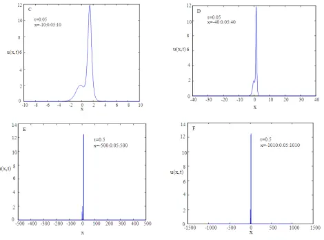
Fig 2.2. (Graphs A-F)2-Soliton Solutions (2SS) at various distances

3. Conclusion

The study of human arterial pulse waves is synonymous with the study of the cardio-vascular system. Waveforms that conform to normal arterial morphology are said to be

physiological. Mathematical models of pressure and flow point to the KdV equation as a good descriptor of arterial waveforms. To this end, studies on the behavior of the solution of the equation, with the aim of providing a clue to clinical needs are engaging much attention. The soliton solutions of the equation have shown that arterial waveforms behave like solitons, true in every sense. The need to obtain multi- soliton solutions therefore arises. It is when such solutions are obtained that a better understanding of the behavior pulse-induced signals and a good prognosis may be achieved. Varieties of algebraic methods that yield solitons were mentioned here; the tanh method and the bilinearmethod were considered for further analysis. We saw that the superposition of solitons is achievable, especially by using the bilinear method of solution. Therefore, relative ease with which multi-solitons can be constructed resides in the bilinear method. The multisolitons obtainable from this method can help in wave-based signaling of the patho-physiological condition of a human subject.

References

[1] T. Laleg, E. Crespeau, and M. Sorine, “Separation of arterial pressure into solitary waves and windkessel flow”, MCBMS’06, IFAC Reims,2006

[2] M.Thiriet, Anatomy and Physiology of the Circulatory And Ventilatory Systems, Springer, 2013.

[3] A. Babin, and A. Figotin, “Linear superposition in nonlinear wave dynamics” Rev. Math. Phys. 18, 971 (2006). DOI: 10.1142/S0129055X06002851,

[4] D. J. Korteweg, and G. de Vries, "On the Change of Form of Long Waves Advancing in a Rectangular Canal, and on a New Type of Long Stationary Waves", Philosophical Magazine 39 (240): 422–443, 1895 doi:10.1080/14786449508620739

[5] T-M. Laleg, E. Crespeau, and M. Sorine, “Seperation of arterial pressure into solitary waves and windkessel flow”, Modeling and Control in Biomedical Systems, Volume 6, Part 1.pp105-110,2006, doi:10.3182/20060920-3-FR-2912.0002

[7] F.E. Nzerem and H.C. Ugorji, “Arterial Pulse Waveform under the watch of Left Ventricular Ejection time: A physiological outlook”, Mathematical Theory and Modeling ,Vol.4, No.4, pp 119-128, 2014

[8] N.J. Zabusky and M.A. Porter, Solition, Scholarpedia, 5(8):2086, 2010.

[9] C. S.Gardner, J. M. Greene, M.D.Kruskal and R.M. Miura, "Method for Solving the Korteweg-deVries Equation", Physical review letters 19: pp 1095–1097, 1967, Bibcode:1967PhRvL..19.1095G,

doi:10.1103/PhysRevLett.19.1095

[10] C. S.Gardner, J. M. Greene, M.D.Kruskal and R.M. Miura,), "Korteweg-deVries equation and generalization. VI. Methods for exact solution", Comm. Pure Appl. Math. 27: pp 97–133, 1974. doi:10.1002/cpa.3160270108, MR 0336122

[11] W. Malfliet, “The tanh method: a tool for solving certain class of nonlinear evolution and wave equations”, J.Comp. Appl. Math. pp 164-165, 2004

[12] W. Malfliet, “Solitary wave solutions of nonlinear wave equations”, Am. J. Phys. 60, pp 650-654, 1992

[13] R. Hirota, “Exact Solution of the Korteweg—de Vries Equation for Multiple Collisions of Solitons”, Phys. Rev.

Lett. 27, 1192, 1971. DOI:

http://dx.doi.org/10.1103/PhysRevLett.27.1192

[14] H. Song and L. Tao, “Soliton solutions for Korteweg-de Vries equation by homotopy analysis method”, AnziamJ (CTAC) pp C152-C158,2008

[15] L. Zou and Z. Zong, “Homotopy analysis method for some nonlinear water wave problems” [Online] http://www.docin.com/p-521846913.html, Retrieved 26May, 2014

[16] W. Hereman and W. Malfliet, “The Tanh Method: atool to solve nonlinear partial differential equations with symbolic software”

[Online]:http://inside.mines.edu/~whereman/papers/Herema n-Malfliet-WMSCI- 2005.pdf retrieved 27May, 2014. [17] J. Hietarinta,” Hirota's bilinear method and soliton

solutions”, Physics AUC, vol.15 (part1), 2005.

[18] J.M. Curry, “Solitions solution of integrable systems and Hirotha’s method”,The Havard college of Mathematics Review 2.1, 2008

[19] W.Hereman, and W. Zhuang, “Symbolic Computation of Solitons via Hirota’s Bilinear Method”. [Online] Available: http://inside.mines.edu/~whereman/papers/Hereman-Zhuang-Hirota- Method-Preprint-1994.pdf