Discriminative Learning of Bayesian Networks via Factorized Conditional Log-Likelihood

Discriminative Learning of Bayesian Networks

via Factorized Conditional Log-Likelihood

Alexandra M. Carvalho [email protected]

Department of Electrical Engineering

Instituto Superior T´ecnico, Technical University of Lisbon INESC-ID, R. Alves Redol 9

1000-029 Lisboa, Portugal

Teemu Roos [email protected]

Department of Computer Science

Helsinki Institute for Information Technology P.O. Box 68

FI-00014 University of Helsinki, Finland

Arlindo L. Oliveira [email protected]

Department of Computer Science and Engineering Instituto Superior T´ecnico, Technical University of Lisbon INESC-ID, R. Alves Redol 9

1000-029 Lisboa, Portugal

Petri Myllym¨aki [email protected]

Department of Computer Science

Helsinki Institute for Information Technology P.O. Box 68

FI-00014 University of Helsinki, Finland

Editor: Russell Greiner

Abstract

We propose an efficient and parameter-free scoring criterion, the factorized conditional log-likelihood (ˆfCLL), for learning Bayesian network classifiers. The proposed score is an ap-proximation of the conditional log-likelihood criterion. The apap-proximation is devised in order to guarantee decomposability over the network structure, as well as efficient estimation of the optimal parameters, achieving the same time and space complexity as the traditional log-likelihood scoring criterion. The resulting criterion has an information-theoretic interpretation based on interaction information, which exhibits its discriminative nature. To evaluate the performance of the proposed criterion, we present an empirical comparison with state-of-the-art classifiers. Results on a large suite of benchmark data sets from the UCI repository show that ˆfCLL-trained classifiers achieve at least as good accuracy as the best compared classifiers, using significantly less computational resources.

Keywords: Bayesian networks, discriminative learning, conditional log-likelihood, scoring

1. Introduction

Bayesian networks have been widely used for classification, see Friedman et al. (1997), Grossman and Domingos (2004), Su and Zhang (2006) and references therein. However, they are often out-performed by much simpler methods (Domingos and Pazzani, 1997; Friedman et al., 1997). One of the likely causes for this appears to be the use of so called generative learning methods in choos-ing the Bayesian network structure as well as its parameters. In contrast to generative learnchoos-ing, where the goal is to be able to describe (or generate) the entire data, discriminative learning focuses on the capacity of a model to discriminate between different classes of instances. Unfortunately, discriminative learning of Bayesian network classifiers has turned out to be computationally much more challenging than generative learning. This led Friedman et al. (1997) to bring up the ques-tion: are there heuristic approaches that allow efficient discriminative learning of Bayesian network classifiers?

During the past years different discriminative approaches have been proposed, which tend to decompose the problem into two tasks: (i) discriminative structure learning, and (ii) discriminative parameter learning. Greiner and Zhou (2002) were among the first to work along these lines. They introduced a discriminative parameter learning algorithm, called the Extended Logistic Regression (ELR) algorithm, that uses gradient descent to maximize the conditional log-likelihood (CLL) of the class variable given the other variables. Their algorithm can be applied to an arbitrary Bayesian net-work structure. However, they only considered generative structure learning methods. Greiner and Zhou (2002) demonstrated that their parameter learning method, although computationally more ex-pensive than the usual generative approach that only involves counting relative frequencies, leads to improved parameter estimates. More recently, Su et al. (2008) have managed to significantly reduce the computational cost by proposing an alternative discriminative parameter learning method, called the Discriminative Frequency Estimate (DFE) algorithm, that exhibits nearly the same accuracy as the ELR algorithm but is considerably more efficient.

Full structure and parameter learning based on the ELR algorithm is a burdensome task. Em-ploying the procedure of Greiner and Zhou (2002) would require a new gradient descent for each candidate network at each search step, turning the method computationally infeasible. Moreover, even in parameter learning, ELR is not guaranteed to find globally optimal CLL parameters. Roos et al. (2005) have showed that globally optimal solutions can be guaranteed only for network struc-tures that satisfy a certain graph-theoretic property, including for example, the naive Bayes and tree-augmented naive Bayes (TAN) structures (see Friedman et al., 1997) as special cases. The work by Greiner and Zhou (2002) supports this result empirically by demonstrating that their ELR algorithm is successful when combined with (generatively learned) TAN classifiers.

For discriminative structure learning, Kontkanen et al. (1998) and Grossman and Domingos (2004) propose to choose network structures by maximizing CLL while choosing parameters by maximizing the parameter posterior or the (joint) log-likelihood (LL). The BNC algorithm of Gross-man and Domingos (2004) is actually very similar to the hill-climbing algorithm of HeckerGross-man et al. (1995), except that it uses CLL as the primary objective function. Grossman and Domingos (2004) also experiment with full structure and parameter optimization for CLL. However, they found that full optimization does not produce better results than those obtained by the much simpler approach where parameters are chosen by maximizing LL.

classifiers. We mostly focus on structure learning. Compared to the work of Grossman and Domin-gos (2004), our structure learning criteria have the advantage of being decomposable, a property that enables the use of simple and very efficient search heuristics. For the sake of simplicity, we assume a binary valued class variable when deriving our results. However, the methods are directly applicable to multi-class classification, as demonstrated in the experimental part (Section 5).

Our first criterion is the approximated conditional log-likelihood (aCLL). The proposed score is the minimum variance unbiased (MVU) approximation to CLL under a class of uniform priors on certain parameters of the joint distribution of the class variable and the other attributes. We show that for most parameter values, the approximation error is very small. However, the aCLL criterion still has two unfavorable properties. First, the parameters that maximize aCLL are hard to obtain, which poses problems at the parameter learning phase, similar to those posed by using CLL directly. Second, the criterion is not well-behaved in the sense that it sometimes diverges when the parameters approach the usual relative frequency estimates (maximizing LL).

In order to solve these two shortcomings, we devise a second approximation, the factorized conditional log-likelihood (ˆfCLL). The ˆfCLL approximation is uniformly bounded, and moreover, it is maximized by the easily obtainable relative frequency parameter estimates. The ˆfCLL criterion allows a neat interpretation as a sum of LL and another term involving the interaction information between a node, its parents, and the class variable; see Pearl (1988), Cover and Thomas (2006), Bilmes (2000) and Pernkopf and Bilmes (2005).

To gauge the performance of the proposed criteria in classification tasks, we compare them with several popular classifiers, namely, tree augmented naive Bayes (TAN), greedy hill-climbing (GHC), C4.5, k-nearest neighbor (k-NN), support vector machine (SVM) and logistic regression (LogR). On a large suite of benchmark data sets from the UCI repository, ˆfCLL-trained classifiers outperform, with a statistically significant margin, their generatively-trained counterparts, as well as C4.5, k-NN and LogR classifiers. Moreover, ˆfCLL-optimal classifiers are comparable with ELR induced ones, as well as SVMs (with linear, polynomial, and radial basis function kernels). The advantage of ˆfCLL with respect to these latter classifiers is that it is computationally as efficient as the LL scoring criterion, and considerably more efficient than ELR and SVMs.

The paper is organized as follows. In Section 2 we review some basic concepts of Bayesian net-works and introduce our notation. In Section 3 we discuss generative and discriminative learning of Bayesian network classifiers. In Section 4 we present our scoring criteria, followed by experimental results in Section 5. Finally, we draw some conclusions and discuss future work in Section 6. The proofs of the results stated throughout this paper are given in the Appendix.

2. Bayesian Networks

In this section we introduce some notation, while recalling relevant concepts and results concerning discrete Bayesian networks.

Let X be a discrete random variable taking values in a countable set

X

X

X

X

xi1, . . . ,xiri where ri is the number of values Xi can take. The probability that X takes value x is

denoted by P(x), conditional probabilities P(x|z)being defined correspondingly.

(nodes) V , each corresponding to one of the random variables Xi, and edges E representing direct

dependencies between the variables. The (possibly empty) set of nodes from which there is an edge to node Xi is called the set of the parents of Xi, and denoted by ΠXi. For each node Xi, we

denote the number of possible parent configurations (vectors of the parents’ values) by qi, the actual

parent configurations being ordered (arbitrarily) and denoted by wi1, . . . ,wiqi. The parameters,Θ=

{θi jk}i∈{1,...,n},j∈{1,...,qi},k∈{1,...,ri}, determine the local distributions in the network via

PB(Xi=xik|ΠXi =wi j) =θi jk.

The local distributions define a unique joint probability distribution over X given by

PB(X1, . . . ,Xn) = n

∏

PB(Xi|ΠXi).

The conditional independence properties pertaining to the joint distribution are essentially deter-mined by the network structure. Specifically, Xiis conditionally independent of its non-descendants

given its parentsΠXi in G (Pearl, 1988).

Learning unrestricted Bayesian networks from data under typical scoring criteria is NP-hard (Chickering et al., 2004). This result has led the Bayesian network community to search for the largest subclass of network structures for which there is an efficient learning algorithm. First at-tempts confined the network to tree structures and used Edmonds (1967) and Chow and Liu (1968) optimal branching algorithms. More general classes of Bayesian networks have eluded efforts to develop efficient learning algorithms. Indeed, Chickering (1996) showed that learning the struc-ture of a Bayesian network is NP-hard even for networks constrained to have in-degree at most two. Later, Dasgupta (1999) showed that even learning an optimal polytree (a DAG in which there are not two different paths from one node to another) with maximum in-degree two is NP-hard. Moreover, Meek (2001) showed that identifying the best path structure, that is, a total order over the nodes, is hard. Due to these hardness results exact polynomial-time algorithms for learning Bayesian networks have been restricted to tree structures.

Consequently, the standard methodology for addressing the problem of learning Bayesian net-works has become heuristic score-based learning where a scoring criterionφis considered in or-der to quantify the capability of a Bayesian network to explain the observed data. Given data D={y1, . . . ,yN} and a scoring criterionφ, the task is to find a Bayesian network B that

maxi-mizes the scoreφ(B,D). Many search algorithms have been proposed, varying both in terms of the formulation of the search space (network structures, equivalence classes of network structures and orderings over the network variables), and in the algorithm to search the space (greedy hill-climbing, simulated annealing, genetic algorithms, tabu search, etc). The most common scoring criteria are reviewed in Carvalho (2009) and Yang and Chang (2002). We refer the interested reader to newly developed scoring criteria to the works of de Campos (2006) and Silander et al. (2010).

Score-based learning algorithms can be extremely efficient if the employed scoring criterion is decomposable. A scoring criterionφis said to be decomposable if the score can be expressed as a sum of local scores that depends only on each node and its parents, that is, in the form

φ(B,D) =

n

∑

One of the most common criteria is the log-likelihood (LL), see Heckerman et al. (1995):

LL(B|D) =

N

∑

log PB(y1t, . . . ,ynt) = n

∑

qi

∑

ri

∑

Ni jklogθi jk,

which is clearly decomposable.

The maximum likelihood (ML) parameters that maximize LL are easily obtained as the observed frequency estimates (OFE) given by

ˆ θi jk=

Ni jk

Ni j

, (1)

where Ni jkdenotes the number of instances in D where Xi=xikandΠXi =wi j, and Ni j=∑ri_k=1Ni jk.

Plugging these estimates back into the LL criterion yields

c

LL(G|D) =

n

∑

qi

∑

ri

∑

Ni jklog

Ni jk

Ni j

.

The notation with G as the argument instead of B= (G,Θ)emphasizes that once the use of the OFE parameters is decided upon, the criterion is a function of the network structure, G, only.

The LL scoring criterion tends to favor complex network structures with many edges sincec adding an edge never decreases the likelihood. This phenomenon leads to overfitting which is usually avoided by adding a complexity penalty to the log-likelihood or by restricting the network structure.

3. Bayesian Network Classifiers

A Bayesian network classifier is a Bayesian network over X= (X1, . . . ,Xn,C), where C is a class

variable, and the goal is to classify instances(X1, . . . ,Xn)to different classes. The variables X1, . . . ,Xn

are called attributes, or features. For the sake of computational efficiency, it is common to restrict the network structure. We focus on augmented naive Bayes classifiers, that is, Bayesian network classifiers where the class variable has no parents,ΠC=/0, and all attributes have at least the class

variable as a parent, C∈ΠXi for all Xi.

For convenience, we introduce a few additional notations that apply to augmented naive Bayes models. Let the class variable C range over s distinct values, and denote them by z1, . . . ,zs. Recall

that the parents of Xi are denoted byΠXi. The parents of Xiwithout the class variable are denoted

by Π∗_Xi =ΠXi\ {C}. We denote the number of possible configurations of the parent setΠ∗Xi by

q∗_i; hence, q∗_i =∏Xj∈Π∗

Xirj.The j’th configuration ofΠ

∗

Xi is represented by w∗i j, with 1≤ j≤q∗i.

Similarly to the general case, local distributions are determined by the corresponding parameters

P(C=zc) =θc,

P(Xi=xik|Π∗Xi=w∗i j,C=zc) =θi jck.

We denote by Ni jckthe number of instances in the data D where Xi=xik,ΠXi∗ =w∗i jand C=zc.

Moreover, the following short-hand notations will become useful:

Ni j∗k= s

∑

Ni jck, Ni j∗=

ri

∑

s

∑

Ni jck,

Ni jc= ri

∑

Ni jck, Nc=

1 n

n

∑

q∗i

∑

ri

∑

Finally, we recall that the total number of instances in the data D is N. The ML estimates (1) become now

ˆ θc=

Nc

N, and θˆi jck= Ni jck

Ni jc

, (2)

which can again be plugged into the LL criterion:

c

LL(G|D) =

N

∑

log PB(y1t, . . . ,ytn,ct)

=

s

∑

Nclog

Nc

N

+

n

∑

qi

∑

ri

∑

Ni jcklog

Ni jck

Ni jc

!

. (3)

As mentioned in the introduction, if the goal is to discriminate between instances belonging to different classes, it is more natural to consider the conditional log-likelihood (CLL), that is, the probability of the class variable given the attributes, as a score:

CLL(B|D) =

N

∑

log PB(ct|yt1, . . . ,ynt).

Friedman et al. (1997) noticed that the log-likelihood can be rewritten as

LL(B|D) =CLL(B|D) +

N

∑

log PB(yt1, . . . ,ynt). (4)

Interestingly, the objective of generative learning is precisely to maximize the whole sum, whereas the goal of discriminative learning consists on maximizing only the first term in (4). Friedman et al. (1997) attributed the underperformance of learning methods based on LL to the term CLL(B|D)

being potentially much smaller than the second term in Equation (4). Unfortunately, CLL does not decompose over the network structure, which seriously hinders structure learning, see Bilmes (2000); Grossman and Domingos (2004). Furthermore, there is no closed-form formula for optimal parameter estimates maximizing CLL, and computationally more expensive techniques such as ELR are required (Greiner and Zhou, 2002; Su et al., 2008).

4. Factorized Conditional Log-Likelihood Scoring Criterion

The above shortcomings of earlier discriminative approaches to learning Bayesian network clas-sifiers, and the CLL criterion in particular, make it natural to explore good approximations to the CLL that are more amenable to efficient optimization. More specifically, we now set out to construct approximations that are decomposable, as discussed in Section 2.

4.1 Developing a New Scoring Criterion

For simplicity, assume that the class variable is binary, C={0,1}.For the binary case the condi-tional probability of the class variable can then be written as

PB(ct|y1t, . . . ,ytn) =

PB(y1t, . . . ,ynt,ct)

PB(yt1, . . . ,ynt,ct) +PB(y1t, . . . ,ytn,1−ct)

For convenience, we denote the two terms in the denominator as

Ut = PB(yt1, . . . ,ynt,ct) and

Vt = PB(y1t, . . . ,ynt,1−ct), (6)

so that Equation (5) becomes simply

PB(ct |y1t, . . . ,ynt) =

Ut

Ut+Vt

.

We stress that both Ut and Vt depend on B, but for the sake of readability we omit B in the notation.

Observe that while(y1_t, . . . ,yn_t,ct)is the t’th sample in the data set D, the vector(y1t, . . . ,ynt,1−ct),

which we call the dual sample of(y1_t, . . . ,y_tn,ct), may or may not occur in D.

The log-likelihood (LL), and the conditional log-likelihood (CLL) now take the form

LL(B|D) =

N

∑

logUt, and

CLL(B|D) =

N

∑

logUt−log(Ut+Vt).

Recall that our goal is to derive a decomposable scoring criterion. Unfortunately, even though logUt

decomposes, log(Ut+Vt)does not.

Now, let us consider approximating the log-ratio

f(Ut,Vt) =log

Ut

Ut+Vt

,

by functions of the form

ˆ

f(Ut,Vt) =αlogUt+βlogVt+γ,

whereα,β, andγare real numbers to be chosen so as to minimize the approximation error. Since the accuracy of the approximation obviously depends on the values of Ut and Vt as well as the constants α,β, andγ, we need to make some assumptions about Utand Vt in order to determine suitable values

ofα,βandγ. We explicate one possible set of assumptions, which will be seen to lead to a good approximation for a very wide range of Ut and Vt. We emphasize that the role of the assumptions is

to aid in arriving at good choices of the constantsα,β, andγ, after which we can dispense with the assumptions—they need not, in particular, hold true exactly.

Start by noticing that Rt =1−(Ut+Vt) is the probability of observing neither the t’th

sam-ple nor its dual, and hence, the trisam-plet(Ut,Vt,Rt)are the parameters of a trinomial distribution. We

assume, for the time being, that no knowledge about the values of the parameters(Ut,Vt,Rt)is

avail-able. Therefore, it is natural to assume that(Ut,Vt,Rt) follows the uniform Dirichlet distribution,

Dirichlet(1,1,1), which implies that

(Ut,Vt)∼Uniform(∆2), (7)

In fact, Ut and Vt are expected to become exponentially small as the number of attributes grows.

Therefore, it is reasonable to assume that

Ut,Vt≤p<

1 2<Rt

for some 0<p<1

2. Combining this constraint with the uniformity assumption, Equation (7), yields the following assumption, which we will use as a basis for our further analysis.

Assumption 1 There exists a small positive p<1

2 such that

(Ut,Vt)∼Uniform(∆2)|Ut,Vt≤p=Uniform([0,p]×[0,p]).

Assumption 1 implies that Ut and Vt are uniform i.i.d. random variables over[0,p]for some

(possibly unknown) positive real number p<1₂. (See Appendix B for an alternative justification for Assumption 1.) As we show below, we do not need to know the actual value of p. Consequently, the envisaged approximation will be robust to the choice of p.

We obtain the best fitting approximation ˆf by the least squares method.

Theorem 1 Under Assumption 1, the values of α, βand γthat minimize the mean square error (MSE) of ˆf w.r.t. f are given by

α = π

2₊₆

24 , (8)

β = π

2₋₁₈

24 ,and (9)

γ = π

2 12 ln 2−

2+(π

2_{−6)log p} 12

, (10)

where log is the binary logarithm and ln is the natural logarithm.

We show that the mean difference between ˆf and f is zero for all values of p, that is, ˆf is unbiased.1 Moreover, we show that ˆf is the approximation with the lowest variance among unbiased ones.

Theorem 2 The approximation ˆf withα,β, γdefined as in Theorem 1 is the minimum variance unbiased (MVU) approximation of f .

Next, we derive the standard error of the approximation ˆf in the square[0,p]×[0,p], which, curiously, does not depend on p. To this end, consider

µ=E[f(Ut,Vt)] =

1 2 ln(2)−2

which is a negative value; as it should since f ranges over(−∞,0].

1. Herein we apply the nomenclature of estimation theory in the context of approximation. Thus, an approximation is unbiased if E[_fˆ_{(Ut,Vt)−f(Ut,Vt)] =0 for all p. Moreover, an approximation is (uniformly) minimum variance}

Theorem 3 The approximation ˆf withα,β, andγdefined as in Theorem 1 has standard error given by

σ=

s

36+36π2₋π4

288 ln2(2) −2≈0.352

and relative standard errorσ/|µ| ≈0.275.

Figure 1 illustrates the function f as well as its approximation ˆf for (Ut,Vt)∈[0,p]×[0,p]with

p=0.05. The approximation error, f−_{f is shown in Figure 2. While the properties established}ˆ in Theorems 1–3 are useful, we find it even more important that, as seen in Figure 2, the error is close to zero except when either Ut or Vt approaches zero. Moreover, we point out that the choice

of p=0.05 used in the figure is not important: having chosen another value would have produced identical graphs except in the scale of the Ut and Vt. In particular, the scale and numerical values on

the vertical axis (i.e., in Figure 2, the error) would have been precisely the same. Using the approximation in Theorem 1 to approximate CLL yields

CLL(B|D) ≈

N

∑

αlogUt+βlogVt+γ

=

N

∑

(α+β)logUt−βlog

Ut

Vt

+γ

= (α+β)LL(B|D)−β

N

∑

log

Ut

Vt

+Nγ, (11)

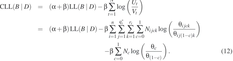
where constantsα,βandγare given by Equations (8), (9) and (10), respectively. Since we want to maximize CLL(B|D), we can drop the constant Nγin the approximation, as maxima are invariant under monotone transformations, and so we can just maximize the following formula, which we call the approximate conditional log-likelihood (aCLL):

aCLL(B|D) = (α+β)LL(B|D)−β

N

∑

log

Ut

Vt

= (α+β)LL(B|D)−β

n

∑

q∗_i

∑

ri

∑

1

∑

Ni jcklog

_θ

i jck θi j(1−c)k

−β 1

∑

Nclog

_θ

c θ(1−c)

. (12)

The fact that Nγcan be removed from the maximization in (11) is most fortunate, as we eliminate the dependency on p. An immediate consequence of this fact is that we do not need to know the actual value of p in order to employ the criterion.

We are now in the position of having constructed a decomposable approximation of the condi-tional log-likelihood score that was shown to be very accurate for a wide range of parameters Ut

and Vt. Due to the dependency of these parameters onΘ, that is, the parameters of the Bayesian

0.00 0.01

0.02 0.03

0.040.05

0.00 0.01 0.02 0.03 0.04 0.05 −6 −4 −2 0 2

Ut

Vt _0.000.01

0.02 0.03

0.040.05

0.00 0.01 0.02 0.03 0.04 0.05 −6 −4 −2 0 2

Ut Vt

Figure 1: Comparison between f(Ut,Vt) =log

Ut Ut+Vt

(left), and ˆf(Ut,Vt) =αlogUt+βlogVt+γ

(right). Both functions diverge (to−∞) as Ut →0. The latter diverges (to+∞) also when

Vt→0. For the interpretation of different colors, see Figure 2 below.

0.00 0.01

0.02 0.03

0.04 0.05

0.00 0.01 0.02 0.03 0.04 0.05 −6 −4 −2 0 2

Ut

Vt −3

−2 −1 0 1 2 3

Figure 2: Approximation error: the difference between the exact value and the approximation given in Theorem 1. Notice that the error is symmetric in the two arguments, and diverges as Ut →0 or Vt →0. For points where neither argument is close to zero, the error is small

is gained by decomposability, it would seem to be dwarfed by the expensive parameter optimization phase.

Furthermore, trying to use the OFE parameters in aCLL may lead to problems since the ap-proximation is undefined at points where either Ut or Vt is zero. To better see why this is the case,

substitute the OFE parameters, Equation (2), into the aCLL criterion, Equation (12), to obtain

ˆaCLL(G|D) = (α+β)LLc(G|D)−β

n

∑

q∗i

∑

ri

∑

1

∑

Ni jcklog

_N

i jckNi j(1−c)

Ni jcNi j(1−c)k

−β 1

∑

Nclog

Nc

N1−c

. (13)

The problems are associated with the denominator in the second term. In LL and CLL cri-teria, similar expressions where the denominator may be zero are always eliminated by the OFE parameters since they are always multiplied by zero, see, for example, Equation (3), where Ni jc=0

implies Ni jck=0. However, there is no guarantee that Ni j(1−c)k is non-zero even if the factors in the

numerator are non-zero, and hence the division by zero may lead to actual indeterminacies.

Next, we set out to resolve these issues by presenting a well-behaved approximation that enables easy optimization of both structure (via decomposability), as well as parameters.

4.2 Achieving a Well-Behaved Approximation

In this section, we address the singularities of aCLL under OFE by constructing an approximation that is well-behaved.

Recall aCLL in Equation (12). Given a fixed network structure, the parameters that maximize the first term,(α+β)LL(B|D), are given by OFE. However, as observed above, the second term may actually be unbounded due to the appearance ofθi j(1−c)kin the denominator. In order to obtain a

well-behaved score, we must therefore make a further modification to the second term. Our strategy is to ensure that the resulting score is uniformly bounded and maximized by OFE parameters. The intuition behind this is that we can thus guarantee not only that the score is well-behaved, but also that parameter learning is achieved in a simple and efficient way by using the OFE parameters— solving both of the aforementioned issues with the aCLL score. As it turns out, we can satisfy our goal while still retaining the discriminative nature of the score.

The following result is of importance in what follows.

Theorem 4 Consider a Bayesian network B whose structure is given by a fixed directed acyclic graph, G. Let f(B|D)be a score defined by

f(B|D) =

n

∑

q∗ i

∑

ri

∑

1

∑

Ni jck

 λlog



 θi jck

Ni jc Ni j∗θi jck+

Ni j(1−c)

Ni j∗ θi j(1−c)k

 



, (14)

whereλis an arbitrary positive real value. Then, the parametersΘthat maximize f(B|D)are given by the observed frequency estimates (OFE) obtained from G.

by the OFE parameters. We will now proceed to determine a suitable value for the parameter λ appearing in Equation (14).

To clarify the analysis, we introduce the following short-hand notations:

A1=Ni jcθi jck, A2=Ni jc,

B1=Ni j(1−c)θi j(1−c)k, B2=Ni j(1−c).

(15)

With simple algebra, we can rewrite the logarithm in the second term of Equation (12) using the above notations as

log

Ni jcθi jck

Ni j(1−c)θi j(1−c)k

−log

Ni jc

Ni j(1−c)

=log

A1 B1

−log

A2 B2

. (16)

Similarly, the logarithm in (14) becomes

λlog

Ni jcθi jck

Ni jcθi jck+Ni j(1−c)θi j(1−c)k

+ρ−λlog

Ni jc

Ni jc+Ni j(1−c)

−ρ

=λlog

A1 A1+B1

+ρ−λlog

A2 A2+B2

−ρ, (17)

where we used Ni j∗=Ni jc+Ni j(1−c); we have introduced the constantρthat was added and

sub-tracted without changing the value of the expression for a reason that will become clear shortly. By comparing Equations (16) and (17), it can be seen that the latter is obtained from the former by replacing expressions of the form log(A

B)by expressions of the formλlog( A A+B) +ρ.

We can simplify the two-variable approximation to a single variable one by taking W = A A+B. In

this case we have that A_B=₁₋W_W, and so we propose to apply once again the least squares method to approximate the function

g(W) =log

W 1−W

by

ˆ

g(W) =λlogW+ρ.

The role of the constantρis simply to translate the approximate function to better match the target g(W).

As in the previous approximation, here too it is necessary to make assumptions about the values of A and B (and thus W ), in order to find suitable values for the parametersλandρ. Again, we stress that the sole purpose of the assumption is to guide in the choice of the parameters.

As both A1, A2, B1, and B2 in Equation (15) are all non-negative, the ratio Wi= _AiAi_+Bi is

al-ways between zero and one, for both i∈ {1,2}, and hence it is natural to make the straightforward assumption that W1 and W2 are uniformly distributed along the unit interval. This gives us the following assumption.

Assumption 2 We assume that

Ni jcθi jck

Ni jcθi jck+Ni j(1−c)θi j(1−c)k

∼ Uniform(0,1), and

Ni jc

Ni jc+Ni j(1−c)

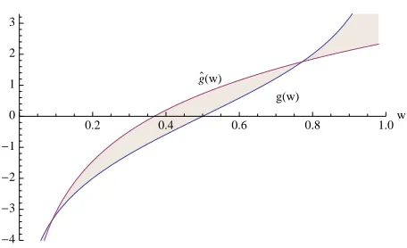
g(w) g`(w)

0.2 0.4 0.6 0.8 1.0w

-4 -3 -2 -1 0 1 2 3

Figure 3: Plot of g(w) =log ₁₋w_wand ˆg(w) =λlog w+ρ.

Herein, it is worthwhile noticing that although the previous assumption was meant to hold for general parameters, in practice, we know in this case that OFE will be used. Hence, Assumption 2 reduces to

Ni jck

Ni j∗k

∼Uniform(0,1), and Ni jc Ni j∗

∼Uniform(0,1).

Under this assumption, the mean squared error of the approximation can be minimized analyti-cally, yielding the following solution.

Theorem 5 Under Assumption 2, the values ofλandρthat minimize the mean square error (MSE) of ˆg w.r.t. g are given by

λ = π

2

6, and (18)

ρ = π

2

6 ln 2. (19)

Theorem 6 The approximation ˆg withλandρdefined as in Theorem 5 is the minimum variance unbiased (MVU) approximation of g.

In order to get an idea of the accuracy of the approximation ˆg, consider the graph of log ₁₋w_w andλlog w+ρin Figure 3. It may appear problematic that the approximation gets worse as w tends to one. However this is actually unavoidable since that is precisely where ˆaCLL diverges, and our goal is to obtain a criterion that is uniformly bounded.

To wrap up, we first rewrite the logarithm of the second term in Equation (12) using for-mula (16), and then apply the above approximation to both terms to get

log

_θ

i jck θi j(1−c)k

≈λlog

Ni jcθi jck

Ni jcθi jck+Ni j(1−c)θi j(1−c)k

+ρ−λlog

Ni jc

Ni j∗

−ρ, (20)

whereρcancels out. A similar analysis can be applied to rewrite the logarithm of the third term in Equation (12) leading to

log

_θ

c θ(1−c)

=log

_θ

c

1−θc

Plugging the approximations of Equations (20) and (21) into Equation (12) gives us finally the factorized conditional log-likelihood (fCLL) score:

fCLL(B|D) = (α+β)LL(B|D)

−βλ

n

∑

q∗_i

∑

ri

∑

1

∑

Ni jck

log

Ni jcθi jck

Ni jcθi jck−Ni j(1−c)θi j(1−c)k

−log

Ni jc

Ni j∗

−βλ 1

∑

Nclogθc−βNρ.

(22)

Observe that the third term of Equation (22) is such that

−βλ 1

∑

Nclogθc=−βλN

1

∑

Nc

N logθc, (23)

and, sinceβ<0, by Gibbs inequality (see Lemma 8 in the Appendix at page 2204) the parameters that maximize Equation (23) are given by the OFE, that is, ˆθc=Nc_N. Therefore, by Theorem 4, given

a fixed structure, the maximizing parameters of fCLL are easily obtained as OFE. Moreover, the fCLL score is clearly decomposable.

As a final step, we plug in the OFE parameters, Equation (2), into the fCLL criterion, Equa-tion (22), to obtain

ˆfCLL(G|D) = (α+β)LLc(B|D)−βλ

n

∑

q∗_i

∑

ri

∑

1

∑

Ni jck

log

Ni jck

Ni j∗k

−log

Ni jc

Ni j∗

−βλ 1

∑

Nclog

Nc

N

−βNρ, (24)

where we also use the OFE parameters in the log-likelihoodLL. Observe that we can drop the lastc two terms in Equation (24) as they become constants for a given data set.

4.3 Information-Theoretical Interpretation

Before we present empirical results illustrating the behavior of the proposed scoring criteria, we point out that the ˆfCLL criterion has an interesting information-theoretic interpretation based on interaction information. We will first rewrite LL in terms of conditional mutual information, and then, similarly, rewrite the second term of ˆfCLL in Equation (24) in terms of interaction information. As Friedman et al. (1997) point out, the local contribution of the i’th variable to LL(B|D)

(recall Equation (3)) is given by

N

q∗_i

∑

1

∑

ri

∑

Ni jck

N log

Ni jck

Ni jc

= −NHPDˆ (Xi|Π∗Xi,C)

= −NHPDˆ (Xi|C) +NIPDˆ (Xi;Π∗Xi |C), (25)

where H_PDˆ (Xi|. . .) denotes the conditional entropy, and I_PDˆ (Xi;Π∗Xi |C) denotes the conditional

theoretic quantities are evaluated under the joint distribution ˆPD of (~X,C) induced by the OFE

parameters.

Since the first term on the right-hand side of (25) does not depend onΠ∗_Xi, finding the parents of Xithat maximize LL(B|D)is equivalent to choosing the parents that maximize the second term,

NI_PDˆ (Xi;Π∗Xi|C), which measures the information thatΠ∗Xi provides about Xiwhen the value of C

is known.

Let us now turn to the second term of the ˆfCLL score in Equation (24). The contribution of the i’th variable in it can also be expressed in information theoretic terms as follows:

−βλN HPDˆ (C|Xi,ΠXi∗)−HPDˆ (C|Π∗Xi)

=βλNIPDˆ (C ; Xi|Π∗Xi)

=βλN I_PDˆ (C ; Xi;Π∗Xi) +I_PDˆ (C ; Xi))

, (26)

where IPDˆ (C ; XI;Π∗Xi)denotes the interaction information (McGill, 1954), or the “co-information”

(Bell, 2003); for a review on the history and use of interaction information in machine learning and statistics, see Jakulin (2005).

Since IPDˆ (Xi; C)on the last line of Equation (26) does not depend onΠ∗Xi, finding the parents of

Xithat maximize the sum amounts to maximizing the interaction information. This is intuitive, since

the interaction information measures the increase—or the decrease, as it can also be negative—of the mutual information between Xiand C when the parent setΠ∗Xi is included in the model.

All said, the ˆfCLL criterion can be written as

ˆfCLL(G|D) =

n

∑

(α+β)NIPDˆ (Xi;Π∗Xi|C)−βλNIPDˆ (C ; Xi;Π∗Xi)

+const, (27)

where const is a constant independent of the network structure and can thus be omitted. To get a concrete idea of the trade-off between the first two terms, the numerical values of the constants can be evaluated to obtain

ˆfCLL(G|D)≈

n

∑

0.322 NIPDˆ (Xi;Π∗Xi |C) +0.557 NIPDˆ (C ; Xi;Π∗Xi)

+const. (28)

Normalizing the weights shows that the first term that corresponds to the behavior of the LL crite-rion, Equation (25), has proportional weight of approximately 36.7 percent, while the second term that gives ˆfCLL criterion its discriminative nature has the weight 63.3 percent.2

In addition to the insight provided by the information-theoretic interpretation of ˆfCLL, it also provides a practically most useful corollary: the ˆfCLL criterion is score equivalent. A scoring criterion is said to be score equivalent if it assigns the same score to all network structures encoding the same independence assumptions, see Verma and Pearl (1990), Chickering (2002), Yang and Chang (2002) and de Campos (2006).

Theorem 7 The ˆfCLL criterion is score equivalent for augmented naive Bayes classifiers.

The practical utility of the above result is due to the fact that it enables the use of powerful algorithms, such as the tree-learning method by Chow and Liu (1968), in learning TAN classifiers.

4.4 Beyond Binary Classification and TAN

Although ˆaCLL and ˆfCLL scoring criteria were devised having in mind binary classification tasks, their application in multi-class problems is straightforward.3 For the case of ˆfCLL, the expression (24) does not involve the dual samples. Hence, it can be trivially adapted for non-binary classifica-tion tasks. On the other hand, the score ˆaCLL in Equaclassifica-tion (13) does depend on the dual samples. To adapt it for multi-class problems, we considered Ni j(1−c)k=Ni j∗k−Ni jckand Ni j(1−c)=Ni j−Ni jc.

Finally, we point out that despite being derived under the augmented naive Bayes model, the ˆfCLL score can be readily applied to models where the class variable is not a parent of some of the attributes. Hence, we can use it as a criterion for learning more general structures. The empirical results below demonstrate that this indeed leads to good classifiers.

5. Experimental Results

We implemented the ˆfCLL scoring criterion on top of the Weka open-source software (Hall et al., 2009). Unfortunately, the Weka implementation of the TAN classifier assumes that the learning criterion is score equivalent, which rules out the use of our ˆaCLL criterion. Non-score-equivalent criteria require the Edmonds’ maximum branchings algorithm that builds a maximal directed span-ning tree (see Edmonds 1967, or Lawler 1976) instead of an undirected one obtained by the Chow-Liu algorithm (Chow and Chow-Liu, 1968). Edmonds’ algorithm had already been implemented by some of the authors (see Carvalho et al., 2007) using Mathematica 7.0 and the Combinatorica package (Pemmaraju and Skiena, 2003). Hence, the ˆaCLL criterion was implemented in this environment. All source code and the data sets used in the experiments, can be found at fCLL web page.4

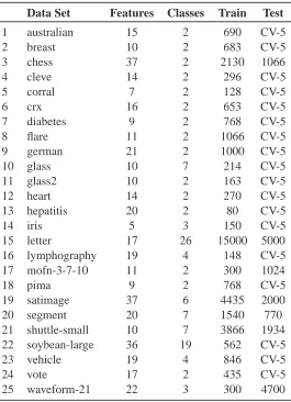
We evaluated the performance of ˆaCLL and ˆfCLL scoring criteria in classification tasks compar-ing them with state-of-the-art classifiers. We performed our evaluation on the same 25 benchmark data sets used by Friedman et al. (1997). These include 23 data sets from the UCI repository of Newman et al. (1998) and two artificial data sets, corral and mofn, designed by Kohavi and John (1997) to evaluate methods for feature subset selection. A description of the data sets is presented in Table 1. All continuous-valued attributes were discretized using the supervised entropy-based method by Fayyad and Irani (1993). For this task we used the Weka package.5 Instances with missing values were removed from the data sets.

The classifiers used in the experiments were:

GHC2: Greedy hill climber classifier with up to 2 parents. TAN: Tree augmented naive Bayes classifier.

C4.5: C4.5 classifier.

k-NN: k-nearest neighbor classifier, with k=1,3,5. SVM: Support vector machine with linear kernel.

SVM2: Support vector machine with polynomial kernel of degree 2.

3. As suggested by an anonymous referee, the techniques used in Section 4.1 for deriving the ˆaCLL criterion can be generalized to the multi-class case as well as to other distributions in addition to the uniform one in a straightforward manner by applying results from regression theory. We plan to explore such generalizations of both the ˆaCLL and ˆfCLL criteria in future work.

4. fCLL web page is athttp://kdbio.inesc-id.pt/˜asmc/software/fCLL.html.

Data Set Features Classes Train Test

1 australian 15 2 690 CV-5

2 breast 10 2 683 CV-5

3 chess 37 2 2130 1066

4 cleve 14 2 296 CV-5

5 corral 7 2 128 CV-5

6 crx 16 2 653 CV-5

7 diabetes 9 2 768 CV-5

8 flare 11 2 1066 CV-5

9 german 21 2 1000 CV-5

10 glass 10 7 214 CV-5

11 glass2 10 2 163 CV-5

12 heart 14 2 270 CV-5

13 hepatitis 20 2 80 CV-5

14 iris 5 3 150 CV-5

15 letter 17 26 15000 5000

16 lymphography 19 4 148 CV-5

17 mofn-3-7-10 11 2 300 1024

18 pima 9 2 768 CV-5

19 satimage 37 6 4435 2000

20 segment 20 7 1540 770

21 shuttle-small 10 7 3866 1934

22 soybean-large 36 19 562 CV-5

23 vehicle 19 4 846 CV-5

24 vote 17 2 435 CV-5

25 waveform-21 22 3 300 4700

Table 1: Description of data sets used in the experiments.

SVMG: Support vector machine with Gaussian (RBF) kernel. LogR: Logistic regression.

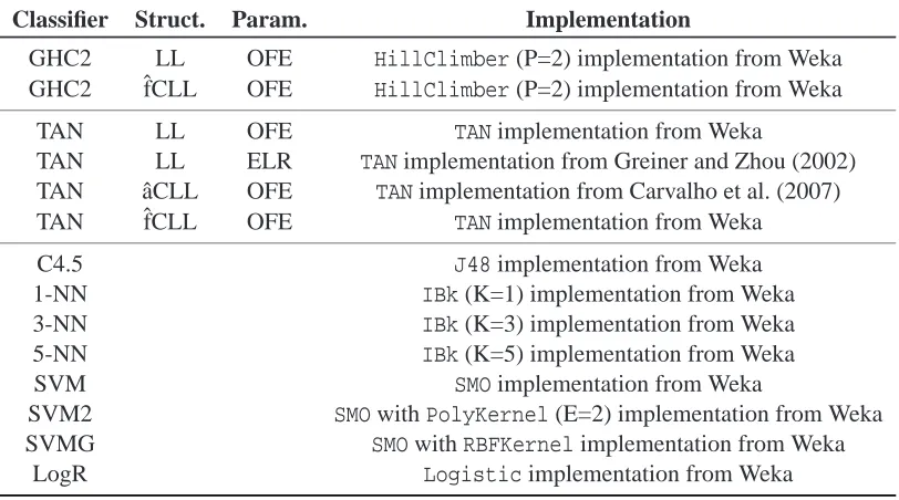
Bayesian network-based classifiers (GHC2 and TAN) were included in different flavors, dif-fering in the scoring criterion used for structure learning (LL, ˆaCLL, ˆfCLL) and the parameter estimator (OFE, ELR). Each variant along with the implementation used in the experiments is de-scribed in Table 2. Default parameters were used in all cases unless explicitly stated. Excluding TAN classifiers obtained with the ELR method, we improved the performance of Bayesian network classifiers by smoothing parameter estimates according to a Dirichlet prior (see Heckerman et al., 1995). The smoothing parameter was set to 0.5, the default in Weka. The same strategy was used for TAN classifiers implemented in Mathematica. For discriminative parameter learning with ELR, parameters were initialized to the OFE values. The gradient descent parameter optimization was terminated using cross tuning as suggested in Greiner et al. (2005).

Classifier Struct. Param. Implementation

GHC2 LL OFE HillClimber(P=2) implementation from Weka

GHC2 ˆfCLL OFE HillClimber(P=2) implementation from Weka

TAN LL OFE TANimplementation from Weka

TAN LL ELR TANimplementation from Greiner and Zhou (2002) TAN ˆaCLL OFE TANimplementation from Carvalho et al. (2007)

TAN ˆfCLL OFE TANimplementation from Weka

C4.5 J48implementation from Weka

1-NN IBk(K=1) implementation from Weka

3-NN IBk(K=3) implementation from Weka

5-NN IBk(K=5) implementation from Weka

SVM SMOimplementation from Weka

SVM2 SMOwithPolyKernel(E=2) implementation from Weka

SVMG SMOwithRBFKernelimplementation from Weka

LogR Logisticimplementation from Weka

Table 2: Classifiers used in the experiments.

function) kernel of the form K(xi,xj) =exp(−γ||xi−xj||2). Following established practice (see

Hsu et al., 2003), we used a grid-search on the penalty parameter C and the RBF kernel parameter γ, using cross-validation. For linear and polynomial kernels we selected C from[10−1,1,10,102]

by using 5-fold cross-validation on the training set. For the RBF kernel we selected C andγfrom

[10−1,1,10,102]and[10−3,10−2,10−1,1,10], respectively, by using 5-fold cross-validation on the training set.

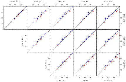
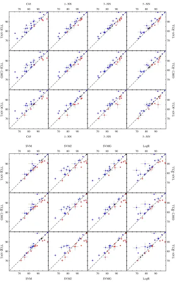
The accuracy of each classifier is defined as the percentage of successful predictions on the test sets in each data set. As suggested by Friedman et al. (1997), accuracy was measured via the holdout method for larger training sets, and via stratified five-fold cross-validation for smaller ones, using the methods described by Kohavi (1995). Throughout the experiments, we used the same cross-validation folds for every classifier. Scatter plots of the accuracies of the proposed methods against the others are depicted in Figure 4 and Figure 5. Points above the diagonal line represent cases where the method shown in the vertical axis performs better than the one on the horizontal axis. Crosses over the points depict the standard deviation. The standard deviation is computed according to the binomial formulapacc×(1−acc)/m, where acc is the classifier accuracy and, for the cross-validation tests, m is the size of the data set. For the case of holdout tests, m is the size of the test set. Tables with the accuracies and standard deviations can be found at the fCLL webpage.

Figure 4: Scatter plots of the accuracy of Bayesian network-based classifiers.

of classifiers. The arrow points towards the learning algorithm that yields superior classification performance. A double arrow is used if the difference is significant with p-value smaller than 0.05. Over all, TAN-ˆfCLL-OFE and GHC-ˆfCLL-OFE performed the best (Tables 3–4). They outper-formed C4.5, the nearest neighbor classifiers, and logistic regression, as well as the generatively-trained Bayesian network classifiers, TAN-LL-OFE and GHC-LL-OFE, all differences being sta-tistically significant at the p<0.05 level. On the other hand, TAN-ˆaCLL-OFE did not stand out compared to most of the other methods. Moreover, TAN-ˆfCLL-OFE and GHC-ˆfCLL-OFE classi-fiers fared sightly better than TAN-LL-ELR and the SVM classiclassi-fiers, although the difference was not statistically significant. In these cases, the only practically relevant factor is computational efficiency.

To roughly characterize the computational complexity of learning the various classifiers, we measured the total time required by each classifier to process all the 25 data sets.6 Most of the methods only took a few seconds (∼1−3 seconds), except for TAN-ˆaCLL-OFE which took a few minutes (∼2−3 minutes), SVM with linear kernel which took some minutes (∼17−18 minutes), TAN-LL-ELR and SVM with polynomial kernel which took a few hours (∼1−2 hours) and, finally, logistic regression and SVM with RBF kernel which took several hours (∼18−32 hours). In the case of TAN-ˆaCLL-OFE, the slightly increased computation time was likely caused by the Mathematica package, which is not intended for numerical computation. In theory, the computational complexity of TAN-ˆaCLL-OFE is of the same order as TAN-LL-OFE or

Classifier GHC2 TAN GHC2 TAN TAN

Struct. ˆfCLL ˆaCLL LL LL LL

Param. OFE OFE OFE OFE ELR

TAN 0.37 1.44 2.13 2.13 0.31

ˆfCLL 0.36 0.07 0.02 0.02 0.38

OFE ← ← ⇐ ⇐ ←

GHC2 1.49 2.26 2.21 0.06

ˆfCLL 0.07 0.01 0.01 0.48

OFE ← ⇐ ⇐ ←

TAN 0.04 -0.34 -1.31

ˆaCLL 0.48 0.37 0.10

OFE ← ↑ ↑

Table 3: Comparison of the Bayesian network classifiers against each other, using the Wilcoxon signed-rank test. Each cell of the array gives the Z-score (top) and the corresponding p-value (middle). Arrow points towards the better method, double arrow indicates statistical significance at level p<0.05.

Classifier C4.5 1-NN 3-NN 5-NN SVM SVM2 SVMG LogR

TAN 3.00 2.25 2.16 2.07 0.43 0.61 0.21 1.80

ˆfCLL <0.01 0.01 0.02 0.02 0.33 0.27 0.42 0.04

OFE ⇐ ⇐ ⇐ ⇐ ← ← ← ⇐

GHC2 3.00 2.35 2.20 2.19 0.39 0.74 0.11 1.65

ˆfCLL <0.01 <0.01 0.01 0.01 0.35 0.23 0.45 0.05

OFE ⇐ ⇐ ⇐ ⇐ ← ← ← ⇐

TAN 2.26 1.34 1.17 1.31 -0.40 -0.29 -0.55 1.37

ˆaCLL 0.01 0.09 0.12 0.09 0.35 0.38 0.29 0.09

OFE ⇐ ← ← ← ↑ ↑ ↑ ←

Table 4: Comparison of the Bayesian network classifiers against other classifiers. Conventions identical to those in Table 3.

OFE: O(n2log n)in the number of features and linear in the number of instances, see Friedman et al. (1997).

increases the cost. In our experiments, SVMs were clearly slower than ˆfCLL-based classifiers. Furthermore, in terms of memory, SVMs with polynomial and RBF kernels, as well as logistic regression, required that the available memory was increased to 1 GB of memory, whereas all other classifiers coped with the default 128 MB.

6. Conclusions and Future Work

We proposed a new decomposable scoring criterion for classification tasks. The new score, called factorized conditional log-likelihood, ˆfCLL, is based on an approximation of conditional log-likelihood. The new criterion is decomposable, score-equivalent, and allows efficient estima-tion of both structure and parameters. The computaestima-tional complexity of the proposed method is of the same order as the traditional log-likelihood criterion. Moreover, the criterion is specifically designed for discriminative learning.

The merits of the new scoring criterion were evaluated and compared to those of common state-of-the-art classifiers, on a large suite of benchmark data sets from the UCI repository. Optimal ˆfCLL-scored tree-augmented naive Bayes (TAN) classifiers, as well as somewhat more general structures (referred to above as GHC2), performed better than generatively-trained Bayesian net-work classifiers, as well as C4.5, nearest neighbor, and logistic regression classifiers, with statistical significance. Moreover, ˆfCLL-optimized classifiers performed better, although the difference is not statistically significant, than those where the Bayesian network parameters were optimized using an earlier discriminative criterion (ELR), as well as support vector machines (with linear, polynomial and RBF kernels). In comparison to the latter methods, our method is considerably more efficient in terms of computational cost, taking 2 to 3 orders of magnitude less time for the data sets in our experiments.

Directions for future work include: studying in detail the asymptotic behavior of ˆfCLL for TAN and more general models; combining our intermediate approximation, aCLL, with discriminative parameter estimation (ELR); extending aCLL and ˆfCLL to mixture models; and applications in data clustering.

Acknowledgments

The authors are grateful to the invaluable comments by the anonymous referees. The authors thank Vtor Rocha Vieira, from the Physics Department at IST/TULisbon, for his enthusiasm in cross-checking the analytical integration of the first approximation, and Mrio Figueiredo, from the Elec-trical Engineering at IST/TULisbon, for his availability in helping with concerns that appeared with respect to this work.

The work of AMC and ALO was partially supported by FCT (INESC-ID multiannual funding) through the PIDDAC Program funds. The work of AMC was also supported by FCT and EU FEDER via project PneumoSyS (PTDC/SAU-MII/100964/2008). The work of TR and PM was supported in part by the Academy of Finland (Projects MODEST and PRIME) and the European Commission Network of Excellence PASCAL.

Appendix A. Detailed Proofs

Proof (Theorem 1) We have that

Sp(α,β,γ) = p Z 0 p Z 0 1 p2 log x x+y

−(αlog(x) +βlog(y) +γ)

2 dy dx

= 1

12 ln(2)2(−π

2_(−1+α+β)

+6(2+4α2+4β2−4 ln(2)−2γln(2) +4 ln(2)2_+8γln(2)2_+2γ2_ln2₍₂₎

+β(5−4(2+γ)ln(2)) +α(1+4β−4(2+γ)ln(2)))

−12(α+β)(1+2α+2β−4 ln(2)−2γln(2))ln(p) +12(α+β)2ln2(p)). Moreover,∇.Sp=0 iff

α = π

2₊₆ 24 ,

β = π

2₋₁₈ 24 ,

γ = π

2 12 ln(2)−

2+(π

2_−6)log(p) 12

,

which coincides exactly with (8), (9) and (10), respectively. Now to show that (8), (9) and (10) define a global minimum, takeδ= (αlog(p) +βlog(p) +γ)and notice that

Sp(α,β,γ) = p Z 0 p Z 0 1 p2 log x x+y

−(αlog(x) +βlog(y) +γ)

2 dy dx = 1 Z 0 1 Z 0 1 p2 log px px+py

−(αlog(px) +βlog(py) +γ)

2

p2dy dx

= 1 Z 0 1 Z 0 log x x+y

−(αlog(x) +βlog(y) + (αlog(p) +βlog(p) +γ))

2 dy dx = 1 Z 0 1 Z 0 log x x+y

−(αlog(x) +βlog(y) +δ)

2 dy dx

= S1(α,β,δ).

So, Sphas a minimum at (8), (9) and (10) iff S1has a minimum at (8), (9) and

δ= π

2

12 ln(2)−2.

The Hessian of S1is _

 

4 ln2(2)

2 ln2(2) −

2 ln(2)

2 ln2(2)

4 ln2(2) −

2 ln(2)

− 2 ln(2) −

2

ln(2) 2

and its eigenvalues are

rcle1 =

3+ln2(2) +

q

9+2 ln2(2) +ln(2)4

ln2(2) ,

e2 = 2 ln2(2),

e3 =

3+ln2(2)−

q

9+2 ln2(2) +ln(2)4

ln2(2) ,

which are all positive. Thus, S1has a local minimum in(α,β,δ)and, consequently, Sphas a local

minimum in(α,β,γ). Since∇.Sphas only one zero,(α,β,γ)is a global minimum of Sp.

Proof (Theorem 2) We have that

p Z 0 p Z 0 1 p2 log x x+y

−(αlog(x) +βlog(y) +γ)

dy dx=0

forα,βandγdefined as in (8), (9) and (10). Since the MSE coincides with the variance for any unbiased estimator, the proposed approximation is the one with minimum variance.

Proof (Theorem 3) We have that

v u u u t p Z 0 p Z 0 1 p2 log x x+y

−(αlog(x) +βlog(y) +γ)

2

dy dx=

s

36+36π2₋π4 288 ln2(2) −2

forα,βandγdefined as in (8), (9) and (10), which concludes the proof.

For the proof of Theorem 4, we recall Gibb’s inequality.

Lemma 8 (Gibb’s inequality) Let P(x) and Q(x) be two probability distributions over the same domain, then

∑

P(x)log(Q(x))≤

∑

x

P(x)log(P(x)).

Proof (Theorem 4) We now take advantage of Gibb’s inequality to show that the parameters that maximize the f(B|D)are those given by the OFE. Observe that

f(B|D) = λ

n

∑

q∗ i

∑

ri

∑

1

∑

Ni jcklog

Ni jcθi jck

Ni jcθi jck+Ni j(1−c)θi j(1−c)k

−log

Ni jc

Ni j∗

= K+λ

n

∑

q∗i

∑

ri

∑

Ni j∗k

1

∑

Ni jck

Ni j∗k

log

Ni jcθi jck

Ni jcθi jck+Ni j(1−c)θi j(1−c)k

where K is a constant that does not depend on the parametersθi jck, and therefore, can be ignored.

Moreover, if we take the OFE for the parameters, we have

ˆ θi jck=

Ni jkc

Ni jc

and ˆθi j(1−c)k=

Ni jk(1−c)

N_{i j(1−c)}. By plugging the OFE estimates in (29) we obtain

ˆ

f(G|D) = K+λ

n

∑

q∗_i

∑

ri

∑

Ni j∗c

1

∑

Ni jck

Ni j∗k

log



 Ni jc

Ni jck Ni jc

Ni jcNi jck_{Ni jc} +Ni j(1−c)

Ni j(1−c)k Ni j(1−c)

 

= K+λ

n

∑

qi

∑

ri

∑

Ni j∗k

1

∑

Ni jck

Ni j∗k

log

Ni jck

Ni j∗k

.

According to Gibb’s inequality, this is the maximum value that f(B|D) can attain, and therefore, the parameters that maximize f(B|D)are those given by the OFE.

Proof (Theorem 5) We have that

S(λ,ρ) =

1 Z 0 log x 1−x

−(λlog(x) +ρ)

2

dx=6λ

2₊π2₊₃ρ2_ln2_{(2)−λ π}2₊₆ρ_ln(2)

3 ln2(2) .

Moreover∇.S=0 iff

λ = π₆2,

ρ = _{6 ln}π2₍₂₎,

which coincides with (18) and (19), respectively. The Hessian of S is

4 ln2₍₂₎ −

2 ln(2),

−_ln2₍₂₎ 2

!

with eigenvalues

2+ln2(2)±

q

4+ln4(2)

ln2(2)

which are both positive. Hence, there is only one minimum, and(λ,ρ)is the global minimum.

Proof (Theorem 6) We have that

1 Z 0 log x 1−x

−(λlog(x) +ρ)

dx=0

forλandρdefined as in Equations (18) and (19). Since the MSE coincides with the variance for any unbiased estimator, the proposed approximation is the one with minimum variance.

Assume that X →Y occurs in G1and Y →X occurs in G2and that X→Y is covered, that is,

ΠG1

Y =Π G1

X ∪ {X}. Since we are only dealing with augment naive Bayes classifiers, X and Y are

different from C and so we also haveΠ∗G1

Y =Π

∗G1

X ∪ {X}. Moreover, take G0 to be the graph G1 without the edge X →Y (which is the same as graph G2 without the edge Y→X ). Then, we have thatΠ∗G0

X =Π

∗G0

Y =Π∗G0 and, moreover, the following equalities hold: Π∗G1

X =Π

∗G0_; Π∗G2

Y =Π

∗G0_;

Π∗G1

Y =Π∗G0∪ {X}; Π

∗G2

X =Π∗G0∪ {Y}.

Since ˆfCLL is a local scoring criterion, ˆfCLL(G1|D)can be computed from ˆfCLL(G0|D)taking only into account the difference in the contribution of node Y . In this case, by Equation (27), it follows that

ˆfCLL(G1|D) = ˆfCLL(G0|D)−((α+β)NI_PDˆ (Y ;Π∗G0|C)−βλNI_PDˆ (Y ;Π∗G0;C))

+((α+β)NIPDˆ (Y ;Π ∗G1

Y |C)−βλNIPDˆ (Y ;Π ∗G1

Y ;C))

= ˆfCLL(G0|D) + (α+β)N(I_PDˆ (Y ;Π∗G0∪ {X} |C)−I_PDˆ (Y ;Π∗G0 |C)) −βλN(IPDˆ (Y ;Π∗G0∪ {X};C)−IPDˆ (Y ;Π∗G0;C))

and, similarly, that

ˆfCLL(G2|D) = ˆfCLL(G0|D) + (α+β)N(IPDˆ (X ;Π∗G0∪ {Y} |C)−IPDˆ (X ;Π∗G0 |C)) + −βλN(I_PDˆ (X ;Π∗G0∪ {Y};C)−I_PDˆ (X ;Π∗G0;C)). To show that ˆfCLL(G1|D) =ˆfCLL(G2|D)it suffices to prove that

I_PDˆ (Y ;Π∗G0∪ {X} |C)−I_PDˆ (Y ;Π∗G0 |C) =I_PDˆ (X ;Π∗G0∪ {Y} |C)−I_PDˆ (X ;Π∗G0|C) (30) and that

IPDˆ (Y ;Π∗G0∪ {X};C)−IPDˆ (Y ;Π∗G0;C) =IPDˆ (X ;Π∗G0∪ {Y};C))−IPDˆ (X ;Π∗G0;C). (31) We start by showing (30). In this case, by definition of conditional mutual, we have that

I_PDˆ (Y ;Π∗G0∪ {X} |C)−I_PDˆ (Y ;Π∗G0 |C) =

=H_PDˆ (Y |C) +H_PDˆ (Π∗G0∪ {X} |C)−H_PDˆ (Π∗G0∪ {X,Y} |C)−H_PDˆ (Y |C) + −HPDˆ (Π∗G0 |C) +HPDˆ (Π∗G0∪ {Y} |C)

=−HPDˆ (Π∗G0|C) +HPDˆ (Π∗G0∪ {X} |C) +HPDˆ (Π∗G0∪ {Y} |C)−HPDˆ (Π∗G0∪ {X,Y} |C)

=IPDˆ (X ;Π∗G0∪ {Y} |C)−IPDˆ (X ;Π∗G0 |C). Finally, each term in (31) is, by definition, given by

IPDˆ (Y ;Π∗G0∪ {X};C) = IPDˆ (Y ;Π∗G0∪ {X} |C)−IPDˆ (Y ;Π∗G0∪ {X})

| {z }

E1

IPDˆ (Y ;Π∗G0;C) = IPDˆ (Y ;Π∗G0 |C)−IPDˆ (Y ;Π∗G0)

| {z }

E2

IPDˆ (X ;Π∗G0∪ {Y};C) = IPDˆ (X ;Π∗G0∪ {Y} |C)−IPDˆ (X ;Π∗G0∪ {Y})

| {z }

E3

I_PDˆ (X ;Π∗G0;C) = I_PDˆ (X ;Π∗G0 |C)−I_PDˆ (X ;Π∗G0

| {z }