Exploration in Relational Domains
for Model-based Reinforcement Learning
Tobias Lang [email protected]
Marc Toussaint [email protected]
Freie Universit¨at Berlin
Machine Learning and Robotics Group Arnimallee 7, 14195 Berlin, Germany
Kristian Kersting [email protected]
Fraunhofer Institute for Intelligent Analysis and Information Systems Knowledge Discovery Department
Schloss Birlinghoven, 53754 Sankt Augustin, Germany
Editor:Satinder Baveja
Abstract
A fundamental problem in reinforcement learning is balancing exploration and exploitation. We address this problem in the context of model-based reinforcement learning in large stochastic re-lational domains by developing rere-lational extensions of the concepts of theE3and R-MAX
algo-rithms. Efficient exploration in exponentially large state spaces needs to exploit the generalization of the learned model: what in a propositional setting would be considered a novel situation and worth exploration may in the relational setting be a well-known context in which exploitation is promising. To address this we introduce relational count functions which generalize the classical notion of state and action visitation counts. We provide guarantees on the exploration efficiency of our framework using count functions under the assumption that we had a relational KWIK learner and a near-optimal planner. We propose a concrete exploration algorithm which integrates a practi-cally efficient probabilistic rule learner and a relational planner (for which there are no guarantees, however) and employs the contexts of learned relational rules as features to model the novelty of states and actions. Our results in noisy 3D simulated robot manipulation problems and in domains of the international planning competition demonstrate that our approach is more effective than ex-isting propositional and factored exploration techniques.
Keywords: reinforcement learning, statistical relational learning, exploration, relational transition models, robotics
1. Introduction
Acting optimally under uncertainty is a central problem of artificial intelligence. In reinforcement learning (RL), an agent’s learning task is to find a policy for action selection that maximizes its re-ward over the long run. Model-based approaches learn models of the underlying transition process, usually formalized as Markov decision processes, from the agent’s interactions with the environ-ment. These models are then analyzed to compute optimal plans.
autonomous agent in an unknown environment: the agent can either make use of its current model of the environment to maximize its cumulative reward (that is, to exploit), or sacrifice short-term rewards to gather information about the environment (that is, to explore) in the hope of increasing future long-term return by improving its model. This exploration-exploitation tradeoff has received considerable attention in unstructured, non-relational domains. There exist algorithms which define unique optimal solutions (such as Bayesian reinforcement learning, Poupart et al., 2006) or provably polynomial time solutions (E3, Kearns and Singh, 2002, and R-MAX, Brafman and Tennenholtz, 2002; Strehl et al., 2009) to the exploration-exploitation trade-off problem. However, while they give a clear idea of how in principle exploration and exploitation can be organized, the basic algo-rithms in their original formulation only work on discrete enumerated state spaces. Therefore, we believe that the core scientific problem is not to find new exploration-exploitation theories, but how these principles can be realized on non-trivial representations (representations other than enumer-ated state spaces), and how the generalization and abstraction implicit in non-trivial representations interferes with these exploration-exploitation principles.
The environment of the agent typically contains varying numbers of objects with relations among them. Learning and acting in such large relational domains is a second key challenge in re-inforcement learning. Relational approaches (Getoor and Taskar, 2007) can generalize information about one object to reach conclusions about other objects and thereby exploit the relational structure of natural environments. Such domains are hard—or even impossible—to represent meaningfully using an enumerated or a propositional state space. As an example, consider a hypothetical house-hold robot which, after taken out of the shipping box and turned on, explores autonomously the environment in order to learn how to perform its cleaning chores. Without a compact knowledge representation that supports abstraction and generalization of previous experiences to the current state and potential future states, it seems to be hopeless for such a “robot-out-of-the-box” to ex-plore one’s home in reasonable time. For instance, after having opened one or two water-taps in bathrooms, the priority for exploring further water-taps in bathrooms, and also in other rooms such as the kitchen, should be reduced. Generalization over object types is crucial for any autonomous agent in realistic environments, but cannot be expressed in a propositional setting where every new object implies a new and therefore non-modeled situation.
The problem of exploration in stochastic relational worlds has so far received little attention. State-of-the-art relational reinforcement learning approaches (Dˇzeroski et al., 2001; Driessens et al., 2006) are mostly model-free and useε-greedy exploration which does not make use of relational knowledge. Exploiting the relational knowledge for exploration is the problem we address in the current paper. Applying existing, propositional exploration techniques is likely to fail: what in a propositional setting would be considered a novel situation and worth exploration may in the rela-tional setting be an instance of a well-known abstract context in which exploitation is promising. In other terms, the key idea underlying our approach is:The inherent generalization of learned knowl-edge in the relational representation has profound implications also on the exploration strategy.
1.1 Our Approach
instan-tiation in this setting where the learner and planner components are based on previous work: The learner is a relational learning algorithm of noisy indeterministic deictic (NID) rules (Pasula et al., 2007) which extracts a compact stochastic relational rule-based model from experience. As a plan-ner we employ PRADA (Lang and Toussaint, 2010) which translates the learned relational model to a grounded dynamic Bayesian network (DBN) and uses approximate inference (a factored frontier) to estimate the expected return of sampled action sequences. Given a learner and a planner, the re-lational exploration-exploitation strategy needs to realize an estimation of novelty in the rere-lational setting. The classical way to estimate state novelty is based on state (and action) visitation counts which, in an enumerated representation, directly reflect model certainty. We generalize the notion of state counts to relational count functions such that visitation of a single state increases this measure of knownness also for “related” states. What is considered related depends on the choice of features used to model these count functions: similar to density estimation with mixtures we assume count functions to be a mixture of basic (relational) features. The inherent generalization in these count functions thus depends on the choice of features. We propose several possible choices of such fea-tures in a relational setting, including one that exploits the specific relational context feafea-tures that are implicitly learned by the relational rule learner.
Ideally, we would like the learner to fulfill guarantees in the KWIK (knows what it knows) framework (Li et al., 2011) and the planner to guarantee near-optimality (in our case, exact in-ference in the corresponding DBN). Clearly, our specific choices for the learner and planner do
not fulfill these guarantees but target at being efficient in challenging applications as we demon-strate in the experimental section. Nevertheless, we will establish theoretical guarantees of our relational exploration-exploitation strategy under the assumption that we had a KWIK learner and near-optimal planning. This will allow us to draw clear connections (i) to the basic R-MAX and
E3 framework for exploration in reinforcement learning and(ii)to the pioneering work of Walsh (2010) on KWIK learning in a relational reinforcement learning setting.
Walsh’s work proved the existence of a KWIK learning algorithm in a relational RL setting by nesting several KWIK algorithms for learning different parts of relational transition models. As Walsh points out himself, however, such an integrated KWIK learner, allowing provably effi-cient exploration, has never been realized or tested and would be “clearly approaching the edge of tractability” (Walsh, 2010). Further, his conceptual algorithm makes limiting assumptions on the model representation which are violated by the more general relational rule framework of Pasula et al. (2007). This is the reason why we choose a practically efficient but heuristic learner which has not been proven to be a KWIK learner. Similarly, it is clear that the computational complexity ofoptimalplanning or exact inference in our corresponding DBN is exponential in the number of objects. Therefore, we choose a practically efficient approximate inference technique for planning in relational domains, as given by PRADA.
1.2 Related Work
optimal solution in a Bayesian framework by taking all potential models weighted by their poste-riors into account at once. This solution is intractable in all but small problem settings, although there have been advances recently such as the near-Bayesian approach by Kolter and Ng (2009). An alternative approach to optimal exploration are algorithms studied in the probabilistically ap-proximately correct (PAC) framework applied to Markov decision processes (MDPs) (so called PAC-MDP approaches). The seminal algorithmsE3(Kearns and Singh, 2002) and R-MAX (Braf-man and Tennenholtz, 2002; Strehl et al., 2009) execute near-optimal actions in all but a polynomial number of steps (or, in alternative problem formulations, only require a polynomial number of steps before they return a near-optimal policy for the current state). Despite the theoretical guarantees of these algorithms, in practice the required exploration steps are often unrealistically large. More importantly, these approaches are designed for enumerated representations of finite domains and thus difficult to apply in domains of everyday life involving many objects.
E3has been extended to parameter learning in factored propositional MDPs with a known struc-ture (Kearns and Koller, 1999) and to MetricE3(Kakade et al., 2003) for state spaces where a metric allows to construct accurate local models. Both approaches assume the existence of efficient near-optimal planning algorithms. However, general algorithms with the required guarantees are not known. Supposedly, this is among the reasons why both approaches have not been empirically demonstrated: “it is thus unlikely that the FactoredE3[for parameter learning] can ever be feasibly implemented” (Guestrin et al., 2002); similar statements can be made for Metric E3. Therefore, Guestrin et al. (2002) propose an exploration strategy for factored propositional MDPs which is tailored towards a specific planning algorithm based on linear programming. The idea of character-izing relevant subspaces for exploration has been pursued in continuous domains using dimension-ality reduction methods (Nouri and Littman, 2010). R-MAXhas been extended to continuous MDPs with linearly parameterized dynamics (Strehl and Littman, 2007). All approaches discussed so far as well as other function approximation methods are propositional, that is, they do not generalize over object types. This can only be achieved by incorporating relational features (which subsume attributes of individual objects), which has not been pursued in the mentioned methods.
relational exploration strategies were not developed. Generally, model-free RL approaches are not suited to realize the type of planned exploration as exemplified in R-MAX, E3 or Bayesian RL. Croonenborghs et al. (2007) learn a relational world model online and additionally use lookahead trees to give the agent more informed Q-values by looking some steps into the future when select-ing an action. Exploration is based on samplselect-ing random actions instead of informed exploration. Diuk (Diuk, 2010; Diuk et al., 2008) presents an algorithm for efficient exploration under certain assumptions in an alternative object-oriented representation of MDPs focused on object attributes. This representation does not account for noisy dynamics in realistic domains where actions may have a large number of low-probability effects. Efficient planning algorithms for this representation still need to be developed.
The pioneering work of Walsh (Walsh, 2010; Walsh et al., 2009; Walsh and Littman, 2008) provides the first principled investigation into the exploration-exploitation tradeoff in relational do-mains. His work lifts ideas from R-MAXand efficient RL algorithms for feature selection (such as the algorithms by Diuk et al., 2009) to relational domains. Walsh establishes sample complexity bounds for specific relational MDP learning problems which scale polynomially in the relational action operator descriptions and the number of objects—in contrast to the original R-MAXandE3
which scale exponentially in the number of objects in relational domains due to the corresponding exponential state and action spaces. Walsh provides an evaluation for some of his algorithms in settings with 2-3 objects; however, his approaches for learning the effects of actions and, more im-portantly, for learning full action operators have not been demonstrated in practice. Despite their theoretical significance, it is uncertain whether an implementation of these algorithms is feasible; this might show an “inherent limitation of the KWIK-learning paradigm [Walsh’s learning frame-work, discussed below] and likely of online learning itself” (Walsh, 2010). Furthermore, to derive theoretical guarantees Walsh assumes a limited language to represent the learned model. Our ap-proach will use the more expressive language of relational NID rules (Pasula et al., 2007), which are necessary to capture the dynamics in realistic domains, for which Walsh’s algorithms would not be applicable. We will detail the differences in representations in Section 3.4.
There is also an increasing number of (approximate) dynamic programming approaches for solving relational MDPs, see for example Boutilier et al. (2001), Kersting et al. (2004), H¨olldobler et al. (2006), Wang et al. (2008) and Sanner and Boutilier (2009). In contrast to the current paper, however, their work assumes a given model of the world. Recently, Lang and Toussaint (2009) and Joshi et al. (2010) have shown that successful planning typically involves only a small subset of relevant objects or states. This can speed up symbolic dynamic programming significantly. A principled approach to exploration, however, has not been developed. Guestrin et al. (2003) calcu-late approximate value functions for relational MDPs from sampled (grounded) environments and provide guarantees for accurate planning in terms of the number of samples; they do not consider an agent which explores its environment step by step to learn a transition model.
1.3 Contributions
The previous section outlined previous work on (mostly model-free) relational RL, which neglected explicit exploration, and the fundamental work by Walsh et al., which proved existence of KWIK learning in a model-based relational RL setting but falls short of practical applicability. The goal of this work is to propose a practically feasible online relational RL system that integrates efficient exploration in relational domains with fully unknown transition dynamics and learning complete action operators (including contexts, effects, and effect distributions).
Our approach extends Kearns and Singh’s theoretically justified exploration techniqueE3and its successor R-MAXand outperforms existing non-relational techniques in a large number of relevant and challenging problems. More precisely, our contributions are the following:
• We introduce the problem of learning relational count functions which generalize the classical notion of state (action) visitation counts.
• We develop a general relational model-based reinforcement learning framework called REX (short for relational explorer), which lifts the concepts ofE3and R-MAXto relational repre-sentations and uses learned relational count functions to estimate empirical model confidence in the relational RL setting.
• We provide guarantees on the exploration efficiency of the general REXframeworkunder the assumption that we hada relational KWIK learner andwerecapable of near-optimal planning in our domain.
• As a concrete instance of our REX framework, we integrate the state-of-the-art relational planner PRADA (Lang and Toussaint, 2010) and a learner for probabilistic relational rules (Pasula et al., 2007) into our framework. The resulting system is the first practically feasible efficient solution for relational domains with fully unknown transition dynamics.
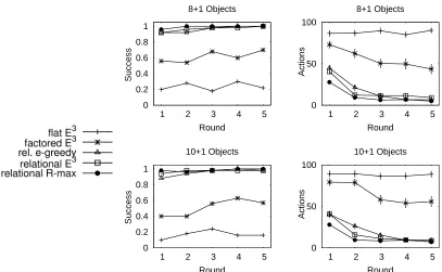
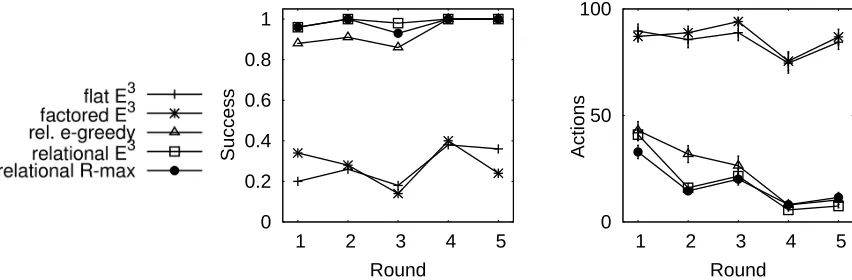
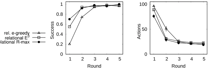
Our extensive experimental evaluation in a 3D simulated complex robot manipulation environment with an articulated manipulator and realistic physics and in domains of the international planning competition (IPPC) shows that our methods can solve tasks in complex worlds where existing propositional methods fail. With these evaluations we also show that relational representations are a promising technique to formalize the idea of curriculum learning (Bengio et al., 2009). Our work has interesting parallels in cognitive science: Windridge and Kittler (2010) employ ideas of relational exploration for cognitive bootstrapping, that is, to progressively learn more abstract rep-resentations of an agent’s environment on the basis of its action capabilities.
1.4 Outline
(a)
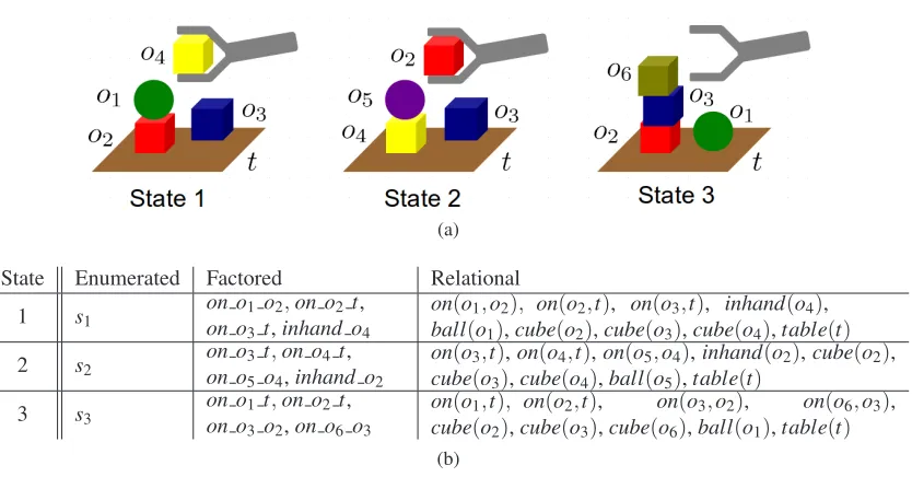
State Enumerated Factored Relational
1 s1
on o1o2,on o2 t,
on o3t,inhand o4
on(o1,o2), on(o2,t), on(o3,t), inhand(o4),
ball(o1),cube(o2),cube(o3),cube(o4),table(t)
2 s2
on o3t,on o4t,
on o5o4,inhand o2
on(o3,t),on(o4,t),on(o5,o4),inhand(o2),cube(o2),
cube(o3),cube(o4),ball(o5),table(t)
3 s3
on o1t,on o2t,
on o3o2,on o6 o3
on(o1,t), on(o2,t), on(o3,o2), on(o6,o3),
cube(o2),cube(o3),cube(o6),ball(o1),table(t) (b)
Table 1: Illustration of three world representation types in a robot manipulation domain
2. Background on MDPs, Representations, Exploration and Transition Models
In this section, we set up the theoretical background for the relational exploration framework and algorithms presented later. First, we review briefly Markov decision processes (MDPs). Then, we describe different methods to represent states and actions in MDPs. Thereafter, we discuss exploration in MDPs including the algorithmsE3and R-MAX. Finally, we discuss in detail compact relational transition models.
2.1 Markov Decision Processes
A Markov decision process (MDP) is a discrete-time stochastic control process used to model the interaction of an agent with its environment. At each time-step, the process is in one of a fixed set of discrete statesSand the agent can choose an action from a setA. The transition modelT specifies the conditional transition distribution P(s′|s,a)over successor states s′ when executing an action
ain a given states. The agent receives rewards in states according to a functionR:S→R≥0(we assume non-negative rewards in this paper without loss of generality). The goal of planning in an MDP is to find a policyπ:S→A, specifying for each state the action to take, which maximizes the expected future rewards. For a discount factor 0<γ<1, the value of a policy πfor a state
s is defined as the expected sum of discounted rewardsVπ(s) =E[∑tγtR(st)|s0=s,π]. In our context, we face the problem of reinforcement learning (RL): we do not know the transition model
T. Without loss of generality, we assume in this paper that the reward functionR is given. We pursue a model-based approach and estimateT from our experiences. Based on our estimate ˆT we compute (approximately) optimal policies.
2.2 State and Action Representations
types dominate AI research on discrete representations:(i)unstructured enumerated representations,
(ii)factored propositional representations, and(iii)relational representations. Table 1 presents three states in a robot manipulation domain together with their translations to the respective representa-tions.
The simplest representation of states and actions is the enumerated (or flat) representation. States and actions are represented by single distinct symbols. Hence, the state and action spaces
SandAare simply enumerated lists. In Table 1, the three states are represented bys1, s2 ands3. This representation cannot capture the structure of states and does not provide a concept of objects. Therefore, it is impossible to express commonalities among states and actions. In the example, all three states appear equally different in this representation.
Afactoredpropositional representation represents a state as a list of attributes. These attributes capture the state structure and hence commonalities among states. MDPs based on factored repre-sentations, called factored MDPs, have been investigated extensively in RL and planning research. The disadvantage of factored representations is their lack of a notion of objects. This makes it im-possible to express commonalities among attributes. For instance, in Table 1 the attributeson o1 o2 andon o5 o4are treated as completely different and therefore State 1 is perceived as equally differ-ent from State 2 as from State 3. Similar argumdiffer-ents hold for actions which are also represdiffer-ented by individual symbols.
Relationalrepresentations account for state structure and objects explicitly. The state spaceS
is described by means of a relational vocabulary consisting of predicates
P
and functionsF
, which yield the set of ground atoms with arguments taken from the set of domain objectsO
. A state is defined by a list of true ground literals. The action spaceAis defined by atomsA
with arguments fromO
. In MDPs based on relational representations, called relational MDPs, the commonalities of state structures, actions and objects can be expressed. They enable compact representations since atoms containing logical variables allow for abstraction from concrete objects and situations. We will speak of grounding an abstract formula ψ if we apply a substitutionσ that maps all of the variables appearing inψto objects inO
. In Table 1, abstract atoms capture the greater similarity of State 1 and State 2 in contrast to the one of State 1 and State 3: we can generalize State 1 and State 2 to the (semi-) abstract stateon(A,B),on(B,table),on(o3,table),inhand(C), which is impossible for State 3.The choice of representation determines the expressivity of models and functions in reinforce-ment learning. In particular, it influences the compactness and generalization of models and the efficiency of learning and exploration as we discuss next.
2.3 Exploration
A central challenge in reinforcement learning is the exploration-exploitation tradeoff. We need to ensure that we learn enough about the environment to accurately understand the domain and to be able to plan for high-value states (explore). At the same time, we have to ensure not to spend too much time in low-value parts of the state space (exploit). The discount factor γof the MDP influences this tradeoff: if states are too far from the agent, the agent does not need to explore them as their potential rewards are strongly discounted; large values forγnecessitate more exploration.
unknown parameters of the MDP. m captures the complexity of the learning problem and cor-responds to the number of parameters of the transition model T in our context. Let Vt(st) =
E[∑∞k=0γkr
t+k|s0,a0,r0. . . ,st]be the value function of the algorithm’s policy (which is non-stationary
and depends on its history), andV∗ of the optimal policy. We define the sample complexity along the lines of Kakade (2003):
Definition 1 Letε>0be a prescribed accuracy andδ>0be an allowed probability of failure. The expressionη(ε,δ,m,γ,Rmax)is asample complexitybound for the algorithm if independently of the choice of s0, with probability at least1−δ, the number of timesteps such that Vt(st)<V∗(st)−εis at mostη(ε,δ,m,γ,Rmax).
An algorithm with a sample complexity polynomial in 1/ε, log(1/δ),m, 1/(1−γ)andRmaxis called
probably approximately correct in MDPs,PAC-MDP(Strehl et al., 2009).
The seminal approach R-MAX(Brafman and Tennenholtz, 2002) provides a PAC-MDP solution to the exploration-exploitation problem in unstructured enumerated state spaces: its sample com-plexity is polynomial in the number of states and actions (Strehl et al., 2009). R-MAXgeneralizes the fundamental approachE3 (Explicit Explore or Exploit) (Kearns and Singh, 2002) for which a similar result has been established in a slightly different formulation:E3finds a near-optimal policy after a number of steps which is polynomial in the number of states and actions. BothE3and R-MAXfocus on the concept ofknown stateswhere all actions have been observed sufficiently often, defined in terms of a thresholdζ. For this purpose, they maintain state-action countsκ(s,a)for all state-action pairs. E3 (Algorithm 1) distinguishes explicitly between exploitation and exploration phases. IfE3enters anunknownstate, it takes the action it has tried the fewest times there (direct ex-ploration). If it enters aknownstate, it tries to calculate a high-value policy within a modelMexploit including all known states with their sufficiently accurate model estimates and a special self-looping state ˜swith zero reward which absorbs unknown state-action pairs (assuming non-negative rewards in the MDP). If it finds a near-optimal policy inMexploitthis policy is executed (exploitation). Oth-erwise,E3plans in a different modelMexplorewhich is equal toMexploitexcept that all known states achieve zero reward and ˜s achieves maximal reward. This “optimism in the face of uncertainty” ensures that the agent explores unknown states efficiently (planned exploration). The value of the known-state threshold ζ depends on several factors: the discount factor γ, the maximum reward
Rmaxand the complexity mof the MDP defined by the number of states and actions as well as the desired accuracyεand confidenceδfor the RL algorithm. The original formulation ofE3assumes knowledge of the optimal value functionV∗to decide for exploitation. Kearns and Singh discuss, however, how this decision can be made without that knowledge. In contrast toE3, R-MAXdecides implicitly for exploration or exploitation and maintains only one modelMR-MAX: it uses its model estimates for the known states, while unknown state-action transitions lead to the absorbing state ˜s
with maximum rewardRmax.
Algorithm 1Sketch ofE3
Input: States
Output: Actiona
1: if∀a:κ(s,a)≥ζthen ⊲State is known
2: Plan inMexploitwith zero-reward for ˜s
3: ifresulting plan has value above some thresholdthen 4: returnfirst action of plan ⊲Exploitation
5: else
6: Plan inMexplorewith maximum reward for ˜sand zero-reward for known states 7: returnfirst action of plan ⊲Planned exploration
8: end if
9: else ⊲State is unknown
10: returnactiona=argminaκ(s,a) ⊲Direct exploration
11: end if
the exploration efficiency and the performance of a reinforcement learning agent. The key idea is to generalize the state-action counts κ(s,a) of the original E3 algorithm over states, actions and objects.
Sample complexity guarantees for more general MDPs can be developed within the KWIK (knows what it knows) framework (Li et al., 2011). In a model-based RL context, a KWIK learning algorithm can be used to estimate the unknown parts of the MDP. This learner accounts for its uncertainty explicitly: instead of being forced to make a prediction (for instance, of the probability of a successor state for a given state-action pair), it can instead signal its uncertainty about the prediction and return a unique symbol⊥. In this case, the (potentially noisy) outcome is provided to the learner which it can use for further learning to increase its certainty. For required model accuracyεand confidenceδ, a model class is calledKWIK-learnableif there is a learner satisfying the following conditions: (1) if the learner does not predict⊥, its prediction isε-accurate, and (2) the number of⊥-predictions is bounded by a polynomial function of the problem description (here, this ismin addition toεandδ). The KWIK-R-MAXalgorithm (Li, 2009) uses a KWIK learner
L
to learn the transition modelT. The predictions ofL
define the known states in the sense ofE3and R-MAX: a state is known if for all actionsL
makesε-accurate predictions (with some failure probability) and unknown otherwise (whereL
predicts⊥). Where the learner is uncertain and predicts⊥, KWIK-R-MAX assumes a transition to ˜s with reward Rmax. Li (2009) shows that ifT can be efficientlyKWIK-learned by
L
, then KWIK-R-MAX usingL
is PAC-MDP. The overall accuracy ε for the sample complexity determines the required individual accuraciesεT for the KWIK model learnerandεP for the planner. Hence, one can derive an efficient RL exploration algorithm by developing
an efficient KWIK learner
L
for the associated model learning problem.2.4 Learning Generalizing Transition Models
The central learning task in model-based reinforcement learning is to estimate a transition model ˆ
T from a set of experiences
E
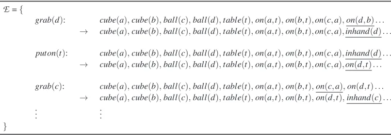
={(st,at,st+1)}Tt=−01 which can be used for decision-making andE ={
grab(d): cube(a),cube(b),ball(c),ball(d),table(t),on(a,t),on(b,t),on(c,a),on(d,b). . . → cube(a),cube(b),ball(c),ball(d),table(t),on(a,t),on(b,t),on(c,a),inhand(d). . .
puton(t): cube(a),cube(b),ball(c),ball(d),table(t),on(a,t),on(b,t),on(c,a),inhand(d). . . → cube(a),cube(b),ball(c),ball(d),table(t),on(a,t),on(b,t),on(c,a),on(d,t). . .
grab(c): cube(a),cube(b),ball(c),ball(d),table(t),on(a,t),on(b,t),on(c,a),on(d,t). . . → cube(a),cube(b),ball(c),ball(d),table(t),on(a,t),on(b,t),on(d,t),inhand(c). . .
..
. ...
}
Table 2: The reinforcement learning agent collects a series
E
of relational state transitions consist-ing of an action (on the left), a predecessor state (first line) and a successor state (second line after the arrow). The changing state features are underlined. The agent uses such experiences to learn a transition model resulting in a compression of the state transitions.This can be achieved by compressing the experiences
E
in a compact model ˆT. Before describing a specific learning algorithm, we discuss conceptual points of learning generalizing models from experience. Compression of the experiences can exploit three opportunities:• The frame assumption states that all state features which are not explicitly changed by an action persist over time. This simplifies the learning problem by deliberately ignoring large parts of the world.
• Abstractionallows to exploit the set of experiences efficiently by means of generalization. It can be achieved with relational representations.
• Assuming uncertainty in the observations is essential to fit a generalizing and regularized function. It allows to tradeoff the exact modeling of every observation (model likelihood) with generalization capabilities and to find low-complexity explanations of our experience: singleton events can be “explained away” as noise. In our point of view, the assumption of uncertainty is crucial to get relational representations working; it “unleashes” the model and opens the door for simplification, abstraction and compactification. Note that even in deter-ministic domains, it may be advantageous to learn a probabilistic model because it can be more abstract, more compact and neglect irrelevant details. In this sense, modeling uncer-tainty can also be understood as regularization.
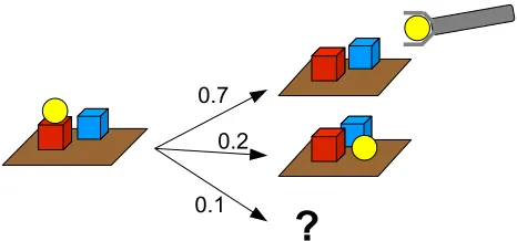
grab(X): on(X,Y),ball(X),cube(Y),table(Z)
→
0.7 : inhand(X),¬on(X,Y) 0.2 : on(X,Z),¬on(X,Y) 0.1 : noise
Table 3: Example NID rule for a robot manipulation scenario, which models to try to grab a ballX. The cubeY is implicitly defined as the one belowX(deictic referencing).X ends up in the robot’s hand with high probability, but might also fall on the table. With a small probability something unpredictable happens. Refer to Figure 1 for an example application.
Figure 1: The NID rule defined in Table 3 can be used to predict the effects of action
grab(speci f ic ball) in the situation on the left side. The right side shows the possible successor states as predicted by the rule. The noise outcome is indicated by a question mark and does not define a unique successor state.
descriptions is simply to provide complex feature descriptors. For instance in Table 2, bothgrab(d) andgrab(c)are used to learn one general model for the abstract actiongrab(X). In turn, the learned model also models situations with previously unseen objects (which is impossible in enumerated and factored propositional representations). In this sense, we view a relational transition model ˆT
as a (noisy) compressor of the experiences
E
whose compactness enables generalization.Transition models which generalize over objects and states play a crucial role in our relational exploration algorithms. While our ideas work with any type of relational model that can be learned from experience, for illustration and to empirically evaluate our ideas we employ noisy indetermin-istic deictic (NID) rules which we present next.
2.4.1 NOISYINDETERMINISTICDEICTICRULES
prediction. Formally, a NID ruleris given as
ar(
X
): φr(X
) →
pr,1 : Ωr,1(
X
) ...
pr,mr : Ωr,mr(
X
) pr,0 : Ωr,0,
where
X
is a set of logic variables in the rule (which represents a (sub-)set of abstract objects). The rule r consists of preconditions, namely that action ar is applied onX
and that the abstract state contextφris fulfilled, andmr+1 different abstract outcomes with associated probabilities pr,i>0,∑i=0pr,i =1. Each outcome Ωr,i(
X
) describes which literals are predicted to change when therule is applied. The context φr(
X
) and outcomesΩr,i(X
)are conjunctions of literals constructedfrom the predicates in
P
as well as equality statements comparing functions fromF
to constant values. The so-called noise outcome Ωr,0 subsumes all possible action outcomes which are not explicitly specified by one of the otherΩr,i. This includes rare and overly complex outcomes whichare typical for noisy domains and which we do not want to cover explicitly for compactness and generalization reasons. For instance, in the context of the rule depicted in Figure 1 a potential, but highly improbable outcome is to grab the blue cube while pushing all other objects off the table: the noise outcome accounts for this without the burden of explicitly stating it. The arguments of the actiona(
X
a)may be a proper subsetX
a⊂X of the variablesX
of the rule. The remaining variables are called deictic referencesDR=X
\X
a and denote objects relative to the agent or action beingperformed.
So, how do we apply NID rules? Let σdenote a substitution that maps variables to constant objects,σ:
X
→O
. Applyingσto an abstract ruler(X
)yields agrounded rule r(σ(X
)). We say a grounded ruler covers a states and a ground action a if s|=φr and a=ar. Let Γbe our setof ground rules andΓ(s,a)⊂Γthe set of rules covering(s,a). If there is a unique covering rule
rs,a∈Γ(s,a) with|Γ(s,a)|=1, we use it to model the effects of actionain states. We calculate P(s′|s,a)by taking all outcomes ofrs,a(omitting subscripts in the following) into account weighted
by their respective probabilities,
P(s′|s,a) = P(s′|s,r) =
mr
∑
i=1
pr,iP(s′|Ωr,i,s) +pr,0P(s′|Ωr,0,s),
where, for i>0, P(s′|Ωr,i,s) =I(s∧Ωr,i|=s′) is a deterministic distribution that is one for the
unique state constructed from staking the changes ofΩr,i into account. (The function I(·)maps
logical truth values to 0 or 1.) The distribution given the noise outcome,P(s′|Ωr,0,s), is unknown and needs to be estimated. Pasula et al. use a worst-case constant boundpmin≤P(s′|Ωr,0,s)to lower boundP(s′|s,a). If a state-action pair(s,a) doesnothave a unique covering ruler (including the case that more than one rule covers the state-action pair, resulting in potentially conflicting predic-tions), we use a noisy default rulerνwhich predicts all effects as noise:P(s′|s,rν) =P(s′|Ωrν,0,s).
their parameters from experience triples
E
={(st,at,st+1)Tt=−01}, relying on the frame assumption. Efficient exploration strategies to collect useful dataE
for learning, however, were not investigated by Pasula et al.—this will be achieved with our proposed methods. The learning algorithm performs a greedy search through the space of rule-sets, maintaining the thus far best performing rule-set. It optimizes the tradeoff between maximizing the likelihood of the experience triples and minimizing the complexity of the current hypothesis rule-setΓby optimizing the scoring metric (Pasula et al., 2007)S(Γ) =
∑
(s,a,s′)
logP(s′|s,rs,a)−α
∑
r∈ΓPEN(r), (1)
wherers,a is either the unique covering rule for(s,a) or the noisy default rulerν. α is a scaling
parameter that controls the influence of regularization. PEN(r)penalizes the complexity of a rule and is defined as the total number of literals in r. The larger α is set, the more compact are the learned rule-sets—and thus, the more general, but potentially also more uncertain and inaccurate. For instance, if we setα=∞, the resulting model will consist of only the default rule, explaining all state transitions as noise. In contrast, if we setα=0, the resulting model explains each experience as accurately as possible, potentially overfitting and not generalizing the data. The learning algo-rithm is initialized with a rule-set comprising only the noisy default rulerνand then iteratively adds
new rules or modifies existing ones using a set of search operators. More precisely, these search operators take the current rule-set and the set of experiences as input, repeatedly select individual rules, modify them with respect to the experiences, and thereby produce new rule-sets. If the best new rule-set scores better than the current rule-set according to Equation (1), it becomes the new rule-set maintained by the algorithm. For instance, the most complex search operator, called Ex-plainExamples, creates new rules from experiences which are modeled by the default rule thus far. First, it builds a complex specific rule for an experience; then, it tries to trim this rule to generalize it to other experiences. Other search operators work directly on existing rules: they add new literals to rule contexts or delete them from contexts, add new deictic references to rules in form of literal sets or delete them, delete complete rules from rule-sets, or generalize comparison literals involving function values in rule contexts.
The noise outcome of NID rules is crucial for learning: it permits the iterative formulation of the learning algorithm as the corresponding noisy default rule covers all experiences without unique covering rule so far; and more importantly, it avoids overfitting by refusing to model rare and overly complex experiences. This advantage has been demonstrated empirically by Pasula et al. (2007). Its drawback is that the successor state distributionP(s′|Ωr,0,s)is unknown. To deal with this problem, the learning algorithm uses a lower bound pmin to approximate this distribution, as
other choices in the learning algorithm (in particular, the choice of search operators and their order) were the same across all reported experiments.
The rule learning algorithm of Pasula et al. uses greedy heuristics in its attempt to learn complete rules. Hence, one cannot give guarantees on its efficiency, correctness or convergence. It has been shown empirically, however, that learned NID rules provide accurate transition models in noisy robot manipulation domains (Pasula et al., 2007; Lang and Toussaint, 2010). In this paper, we show further that the transition dynamics of many domains of the international planning competition can be learned reliably with NID rules. In all our investigated domains, independent learning runs converged to the same or very similar rule-sets; in particular, the learned rule contexts are usually the same.
2.5 Planning with Probabilistic Relational Rules
Model-based RL requires efficient planning for exploitation and planned (directed) exploration. The semantics of NID rules allow one to find a “satisficing” action sequence in relational domains that will lead with high probability to states with large rewards. In this paper, we use thePRADA al-gorithm (Lang and Toussaint, 2010) for planning in grounded relational domains. Empirical results have shown that PRADA finds effective and reliable plans in difficult scenarios. PRADA grounds a given set of abstract NID rules with respect to the objects in the domain and converts the grounded rules to factored dynamic Bayesian networks (DBNs). The random variables (nodes) of the DBNs represent the state literals, actions, rules, rule contexts and outcomes and rewards at different time-steps; factors on these variables define the stochastic transition dynamics according to the NID rules. For planning, PRADA samples sequences of actions in an informed way taking into account the effects of previous actions. To evaluate an action sequence, it uses fast approximate inference to calculate posterior beliefs over states and rewards. If exact instead of approximate inference is used, PRADA is guaranteed to find the optimal plan with high probability given a sufficient number of samples (Lang, 2011). PRADA can plan for different types of rewards, including conjunctions of abstract and grounded literals. Thus, it can be used in model-based RL for both exploiting the learned model to plan for high-reward states as well as for exploring unknown states and actions using theRmax reward. The number of sampled action sequences trades off computation time and plan quality: the more samples are taken, the higher are the chances to find a good plan. In our experiments, we set this number sufficiently high to ensure that good plans are found with high probability. If we know the maximum reward, we can determine PRADA’s planning horizon for a desired level of accuracy from the discount factor γof the MDP: we can calculate after which time-step the remaining maximally possible rewards can be ignored.
3. Exploration in Relational Domains
Relational representations enable generalization of experiences over states, actions and objects. Our contribution in this paper are strategies to exploit this for exploration in model-based reinforcement learning. First, we discuss the implications of a relational knowledge representation for exploration on a conceptual level (Section 3.1). We show how to quantify the knowledge of states and actions by means of a generalized, relational notion of state-action counts, namely arelational count function. This opens the door to a large variety of possible exploration strategies. Thereafter, we propose a relational model-based reinforcement learning framework lifting the ideas of the algorithmsE3
concerning the exploration efficiency in our framework (Section 3.3). Finally, we present a concrete algorithm in this framework which uses some of the previously introduced exploration strategies (Section 3.4), including an illustrative example (Section 3.5).
3.1 Relational Count Functions for Known States and Actions
The theoretical derivations of the efficient non-relational exploration algorithms E3 and R-MAX show that the concept of known states is crucial. On the one hand, the confidence in estimates in known states drives exploitation. On the other hand, exploration is guided by seeking for novel (yet unknown) states and actions. For instance, the direct exploration phase inE3chooses novel actions, which have been tried the fewest; the planned exploration phase seeks to visit novel states, which are labeled as yet unknown.
In the original E3 and R-MAX algorithms operating in an enumerated state space, states and actions are considered known based directly on theircounts: the number of times they have been visited. In relational domains, we should go beyond simply counting state-action visits to estimate the novelty of states and actions:
• The size of the state space is exponential in the number of objects. If we base our notion of known states directly on visitation counts, then the overwhelming majority of all states will be labeled yet-unknown and the exploration time required to meet the criteria for known states ofE3and R-MAXeven for a small relevant fraction of the state space becomes exponential in the number of objects.
• The key benefit of relational learning is the ability to generalize over yet unobserved in-stances of the world based on relational abstractions. This implies a fundamentally different perspective on what is novel and what is known and permits qualitatively different exploration strategies compared to the propositional view.
We propose to generalize the notion of counts to a relational count function that quantifies the degree to which states and actions are known. Similar to using mixtures (e.g., of Gaussians) for density modeling, we model a count function over the state space as a linear superposition of features
fk(“mixture components”) such that visitation of a single state generalizes to “neighboring” states— where “neighboring” is defined by the structure of the features fk. The only technical difference
between count functions and mixture density models is that our count functions are not normalized. Theoretical guarantees on the convergence and accuracy for this model are discussed in Sec-tion 3.3. Given sets of features fk and mixture weights wk, a count function over states scan be
written as
κ(s) =
∑
k
wkfk(s).
The state features fk can be arbitrary. An example for a relational feature are binary tests that
have value 1 if some relational query is true for s; otherwise they have value 0. Estimating such mixture models is a type of unsupervised learning or clustering and involves two problems: finding the features fk themselves (structure learning) and estimating the feature weights wk (parameter
learning).
complexity of features and hence, we have essentially infinitely many features to choose from. The longer a relational feature is (e.g., a long conjunction of abstract literals) and the more variables it contains, the larger is the number of possible ways to bind the variables and the larger is the set of refined features that we potentially have to consider when evaluating a feature. In addition, the space of the instances s is very large in our case. Recall that even very small relational models can have hundreds of ground atoms and it would be impossible to represent all possible states. For instance, for just a single binary relation and 10 objects there would be 100 ground atoms and hence 2100 distinct states, which is clearly intractable. Thus, we need to focus on a compact, structured representation of the count functions. Furthermore, we only have a finite set of positive (that is, experienced) states from which we have to generalize to other states, while taking care not to over-generalize wrongly. Note that in contrast the originalE3and R-MAX algorithms for unstructured domains do not face this problem as they do not generalize experiences to other states. Thus, we essentially face the problem of structure learning from positive examples only (Muggleton, 1997). This is more difficult than the traditional setting considered in relational learning that additionally assumes that negative (impossible) examples are given.
If the features are given, however, the estimation of the count function becomes simpler: only the weights need to be learned. For instance, in 1-class SVMs for density estimation assumptions about the feature structure are embedded in the kernel function; in the mixture of Gaussians model, the functional form of Gaussians is given a-priori and provides the structure. We propose a “patch up” approach in this paper. We examine different choices of features in the relational setting whose weights can be estimated based on empirical counts. While they are only approximations, we then show that we can “patch up” and improve some of these approximations, namely the context-based features (see below) through learning NID rules. In our relational model-based RL algorithms as well as in our evaluation, we focus on context-based features. In other words, our methods implicitly solve both structure and parameter learning from positive examples only.
Let us now introduce different choices of features for the estimation of relational count func-tions. These imply different approaches to quantify known states and actions in a relational RL setting. We focus on a specific type of features, namely queriesq∈Q. Queries are simply relational formulas, for instance conjunctions of ground or abstract literals, which evaluate to 0 or 1 for a given states. We discuss different choices ofQin detail below including examples. Our count functions use queriesqin combination with the set of experiences
E
of the agent and the estimated transition model ˆT. Given a setQof queries we model the state count function asκQ(s) = ∑q∈QcE(q)I(∃σ:s|=σ(q)) (2)
with cE(q) = ∑(se,ae,s′
e)∈E I(∃σ:se|=σ(q)) . (3)
This function combines the confidences of all queriesq∈Qwhich are fulfilled in states. The second term in Equation (2) examines whether queryqis fulfilled ins: the substitutionσis used to ground potentially abstract queries; the functionI(·)maps logical statements to 1 if they are satisfied and to 0 otherwise.cE(q), the first term in Equation (2), is an experience-count of queryq: it quantifies the number of times queryq held in previously experienced predecessor states in the agent’s set of observed state transitions
E
={(st,at,st+1)}tT=−11. Overall, a state s has a high countκQ(s) ifit satisfies queriesq∈Qwith large experience-countscE(q). This implies that all states with low
κQ(s)are considered novel and should be explored, as inE3and R-MAX. The model for state-action
three states shown in Table 1 as our running example: we assume that our experiences consist of exactly State 1, that is
E
={(s1,a1,s′1)} (the actiona1 and the successor states′1 are ignored byκQ(s)), while State 2 and State 3 have not been experienced.
Enumerated: Let us first consider briefly the propositional enumerated setting. We have a finite enumerated state spaceSand action spaceA. The set of queries,
Qenum={s| ∃(se,ae,s′e)∈
E
:se=s},corresponds to predecessor statess∈Swhich have been visited in
E
. Thus, queries are conjunctions of positive and negated ground atoms which fully describe a state. This translates directly to the count functionκenum(s) =cE(s), withcE(s) =
∑
(se,ae,s′e)∈EI(se=s).
The experience-countcE(q)in the previous equation counts the number of occasions stateshas been visited in
E
(in the spirit of Thrun, 1992). There is no generalization in this notion of known states. Similar arguments can be applied on the level of state-action countsκ(s,a). As an illustration, in our running example of Table 1 both State 2 and State 3 are equally unknown and novel: both are not the experienced State 1.Literal-based: Given a relational structure with the set of logical predicates
P
, an alternative approach to describe what are known states is based on counting how often a (ground) literal (a po-tentially negated atom) has been observed true or false in the experiencesE
(all statements equally apply to functionsF
, but we neglect this case here). A literall for a predicateP∈P
containing variables is abstract in that it represents the set of all corresponding ground, that is variable-free, literals forP. Ground literals then play the role of the traditional factors used in mixture models. First, we consider ground literalsl∈L
G with arguments taken from the domain objectsO
. This leads to the set of queriesQlit=L
Gand in turn to the count functionκlit(s) = ∑l∈LG cE(l)I(s|=l) with cE(l):=∑(se,ae,s′
e)∈EI(se|=l).
Each queryl∈
L
Gexamines whetherlhas the same truth values insas in experienced states. This implies that a state is considered familiar (withκlit(s)>0) if a ground literal that is true (false)in this state has been observed true (false) before. Thus abstraction over states can be achieved by means of ground literals. We can follow the same approach for abstract literals
L
Aand setQlit=L
A.Forl∈
L
Aand a states, we examine whether there are groundings of the logical variables inlsuchthatscoversl. More formally, we replaces|=lby∃σ:s|=σ(l). For instance, we may count how often a specific blue ball was on top ofsomeother object. If this was rarely the case this implies a notion of novelty which guides exploration. For example, in Table 1 State 1 and State 3 share the ground literalon(o2,t) while this literal does not hold in State 2. Thus, if Qlit ={on(o2,t)} and State 1 is the sole experienced state, then State 3 is perceived as better known than State 2. In contrast, if we use the abstract queryinhand(X)(expressing there wassomethingheld inhand) and setQlit ={inhand(X)}, then State 3 is perceived as more novel, since in both State 1 and State 2 some object was held inhand. Note that this second query abstracts from the identities of the inhand held objects.
have some notion of context or rule precondition, in our running example of NID rules these may correspond to the set of NID rule contexts{φr}. These are learned from the experiences
E
and havespecifically been optimized to be a compact context representation (cf. Section 2). Given a setΦof such queries, settingQΦ=Φresults in the count function
κΦ(s) = ∑φ∈ΦcE(φ)I(∃σ:s|=σ(φ)) with cE(φ) = ∑(se,ae,s′
e)∈E I(∃σ:se|=σ(φ)).
cE(φ) counts in how many experiences
E
the context respectively query φ was covered with ar-bitrary groundings. Intuitively, contexts may be understood as describing situation classes based on whether the same abstract prediction models can be applied. Taking this approach, states are considered novel if they are not covered by any existing context (κΦ(s) =0) or covered by a contextthat has rarely occurred in
E
(κΦ(s)is low). That is, the description of novelty which drivesexplo-ration is lifted to the level of abstraction of these relational contexts. Similarly, we estimate a count function for known state-action pairs based on state-action contexts. For instance, in the case of a setΓof NID rules, each rule defines a state-action context, resulting in the count
κΦ(s,a) = ∑r∈ΓcE(r)I(r=rs,a), with cE(r) := |
E
(r)|,which is based on counting how many experiences are covered by the unique covering rulers,afor a ins.
E
(r) are the experiences inE
covered by r,E
(r) ={(s,a,s′)∈E
|r=rs,a}. Thus, thenumber of experiences covered by the rulers,a modeling(s,a)can be understood as a measure of
confidence inrs,aand determinesκΦ(s,a). We will useκΦ(s,a)in our proposed algorithm below.
In the example of Table 1, assume in State 1 we perform puton(o3) successfully, that is, we put the inhand cubeo4on o3. From this experience, we learn a rule for the action puton(X)with the contextφ=clear(X)∧inhand(Y). Thereafter, State 3 is perceived as more novel than State 2: the effects ofputon(o3)can be predicted in State 2, but not in State 3.
Similarity-based: Different methods to estimate the similarity of relational states exist. For instance, Driessens et al. (2006) and Halbritter and Geibel (2007) present relational reinforcement learning approaches which use relational graph kernels to estimate the similarity of relational states. These can be used to estimate relational counts which, when applied in our context, would readily lead to alternative notions of novelty and thereby exploration strategies. This count estimation technique bears similarities to MetricE3(Kakade et al., 2003). Applying such a method to model
κ(s)from
E
implies that states are considered novel (with lowκ(s)) if they have a low kernel value (high “distance”) to previous explored states. Letk(·,·)∈[0,1]denote an appropriate kernel for the queriesq∈Q, for instance based on relational graph kernels. We replace the hard indicator functionI(∃σ:s|=σ(q))in Equation (2) by the kernel function, resulting in the more general kernel-based count function
κk,Q(s) = ∑q∈QcE(q)k(s,q).
If one setsQ={s|s∈S}to the set of all states, the previous count function measures the distance to all observed predecessor states multiplied by experience-counts. In the example of Table 1 with
The above approaches are based on counts over the set of experiences
E
. As a simple extension, we propose using thevariabilitywithinE
. Consider two different series of experiencesE
1andE
2 both of sizen. Imagine thatE
1consists ofntimes the same experience, while the experiences inE
2differ. For instance,
E
1might list repeatedly grabbing the same object in the same context, whileE
2might list grabbing different objects in varying conditions.E
2has a higher variability. Although the experience-counts cE1(q) and cE2(q) as defined in Equation (3) are the same, one might betempted to say that
E
2confirmsqbetter as the queryqsucceeded in more heterogeneous situations, supporting the claim of generalization. We formalize this by redefining the experience-counts in Equation (3) using a distance estimated(s,s′)∈[0,1]for two statessands′ascVE(q) =
∑
(st,at,st′)∈E
I(∃σ:st |=σ(q))·δ(st,
E
(q,t)),with
E
(q,t)={(se,ae,s′e)∈E
| ∃σ:se|=σ(q)∧e<t}and δ(s,
E
) = min(se,ae,s′
e)∈E
d(s,se).
The experience-countcVE(q)weights each experience based on its distanceδ(st,
E
(q,t))to priorex-periences (while the original cE(q) assigns all experiences the same weight irrespective of other experiences). Here, the measure d(s,s′) computes the distance between two ground states, but calculations on partial or (partially) lifted states are likewise conceivable. To compute d(s,s′), a kernel k(s,s′)∈[0,1] as above might be employed, d(s,s′)∝1−k(s,s′), for instance using a simple distance estimate based on least general unifiers (Ramon, 2002). For illustration, consider again the states in Table 1. Assume two series of experiences
E
1={(s1,a1,s′1),(s2,a2,s′2)}andE
2={(s1,a1,s′1),(s3,a3,s′3)}and the queryq=on(X,Y)∧ball(X) (that there is a ball on-top of some other object). All State 1, State 2 and State 3 cover this query, therefore the standard counts forE
1andE
2according to Equation (3) are the same,cE1(q) =cE2(q). As State 1 and State 2 sharethe same structure, however, the variability within
E
1is smaller than withinE
2. Thus,E
2provides more heterogeneous evidence forqand thereforecVE2(q)>c
V
E1(q).
3.2 Relational Exploration Framework
The approaches to estimate relational state and action counts which have been discussed above open a large variety of possibilities for concrete exploration strategies. In the following, we derive a re-lational model-based reinforcement learning framework we call REX(short for relational explorer) in which these strategies can be applied. This framework is presented in Algorithm 2. REXliftsE3
and R-MAXto relational exploration.
At each time-step, the relational explorer performs the following general steps:
1. It adapts its estimated relational transition model ˆT with the set of experiences
E
.2. Based on
E
and ˆT, it estimates the count function for known states and actions, κ(s) andκ(s,a). For instance, ˆT might be used to provide formulas and contexts to estimate a specific relational count function.
3. The estimated count function is used to decide for the next actionat based on the strategy of
eitherE3or R-MAX.
Algorithm 2Relational Exploration (REX)
Input: Start states0, reward functionR, confidence thresholdζ 1: Set of experiencesE=/0
2: fort=0,1,2 . . .do
3: Update transition model ˆT according toE
4: Estimateκ(s)andκ(s,a)fromEand ˆT ⊲Relational representation enables generalization 5: ifE3-explorationthen ⊲E3-exploration
6: if∀a∈A:κ(st,a)≥ζthen ⊲State is known→uses relational generalization
7: Plan inMexploitwith zero reward for ˜s ⊲uses relational generalization
8: ifresulting plan has value above some thresholdthen
9: at=first action of plan ⊲Exploitation
10: else
11: Plan inMexplorewith maximum reward for ˜sand zero-reward for known states
12: ⊲uses relational generalization
13: at=first action of plan ⊲Planned exploration
14: end if
15: else ⊲State is unknown
16: at=argminaκ(st,a) ⊲Direct exploration→uses relational generalization
17: end if
18: else ⊲R-MAX-exploration
19: Plan inMR-MAXwith maximum reward for ˜sand given rewardRfor all known states
20: ⊲uses relational generalization
21: at=first action of plan 22: end if
23: Executeat
24: Observe new statest+1
25: Update set of experiencesE←E∪ {(st,at,st+1)}
26: end for
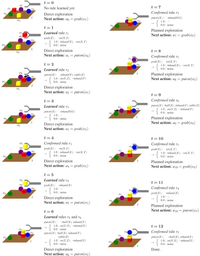
a policy with a sufficiently high value), planned exploration to unknown states is undertaken; otherwise (if the current statest is not known), direct exploration is performed. Like in the original non-relationalE3, the decision for exploitation in relationalE3assumes knowledge of the optimal values. To remove this assumption, the relational explorer can instead attempt planned exploration first along the lines described by Kearns and Singh for the originalE3. In the case of relational R-MAX, a single model is built in which all unknown states according to the estimated counts lead to the absorbing special state ˜swith rewardRmax.
4. Finally, the actionatis executed, the resulting statest+1observed and added to the experiences
E
, and the process repeated.The estimation of relational count functions for known states and actions,κ(s)andκ(s,a), and the resulting generalization over states, actions and objects play a crucial role at several places in the algorithm; for instance, in the case of relationalE3,
• to decide whether the current state is considered known or novel;
• to determine the set of known states where to try to exploit;