Statistical Analysis of Rice Husk Ash as a Construction Material in Building Production Process

(1)

_____________________________________________________________________________________________________

Statistical Analysis of Rice Husk Ash as a

Construction Material in Building Production

Process

John U. Ezeokonkwo

1

,

Chukwuemeka D. Ezeliora

2*

and Echefuna C. Mbanusi

1

1_{Department of Building, Nnamdi Azikiwe University, Awka, Anambra State, Nigeria.}

2

Department of Mechanical Engineering, Nnamdi Azikiwe University, Awka, Anambra State, Nigeria.

Authors’ contributions

This work was carried out in collaboration among all authors. All authors read and approved the final manuscript.

Article Information

DOI: 10.9734/JERR/2019/v5i416931 Editor(s): (1) Dr. Djordje Cica Associate Professor, Faculty of Mechanical Engineering, University of Banja Luka, Bosnia and Herzegovina. Reviewers: (1) Qiang Li, School of Electronic Automaton, Weifang University of Science and Technology, Shandong, China.

(2)J. Dario Aristizabal-Ochoa, Civil Engineering National University of Colombia Medellin, Colombia. (3)Grienggrai Rajchakit, Maejo University, Thailand. Complete Peer review History:http://www.sdiarticle3.com/review-history/47661

Received 20 December 2018 Accepted 03 March 2019 Published 17 June 2019

ABSTRACT

This study considers the statistical analysis of rice husk ash as a construction material in building production process. The quality of concrete mixture is of inevitable concern to all stakeholders in the construction industry in the zone when the climatic conditions of the zone are considered. The mix ratio is examined and all the prevailing construction/production practices are considered statistically. The statistical tools employed are descriptive, normality, process statistical summary and confidence estimation methods of statistics. The tools portrays the necessary information in the data to understand what the data information for further production process analysis.

Keywords: Concrete; quality; production; process; statistics; rice husk; ash.

1. INTRODUCTION

The construction sector plays an active role in the formation of fixed assets in any economy. It

(2)

product. From the above, it has a very high capacity to generate growth and induce multiplier effects in the economy of a nation.

However, current developments in the construction industry in Nigeria are inducing negative effects within the industry. For example, the problem of the collapse of buildings has been persistent in the country in recent times and the need to offer solutions to avoid future events becomes evident. In the last ten years, the incidence of the collapse of buildings has become so alarming and worrisome that it shows no signs of diminishing. Each collapse has tremendous effects that none of its victims can easily forget. These effects include the loss of human lives, economic waste, loss of jobs, income, loss of confidence, dignity and the exasperation of crisis among stakeholders and environmental disasters [2]. It is believed that any search in human life has its cost, but the cost paid in the southeast of Nigeria due to incessant incidents of collapse of buildings cannot be understood or quantified.

Buildings are structures that provide shelter for man, his properties and activities. As such, they must be planned, designed and constructed properly to obtain the desired environmental satisfaction. The main factors observed during the construction of the building include; the functional performance requirements of durability, adequate stability to avoid structural failures, discomfort for users, resistance to weather conditions and use of good quality materials. Building styles of buildings are constantly changing with the introduction of new materials and construction techniques. Consequently, the work involved in the design and construction stages are, to a large extent, those of selection of materials, components and structures that will comply with the standards and aesthetics of construction expected on an economic basis [3].

A general survey shows that most modern buildings in southeastern Nigeria have concrete as their main component. Then, it becomes pertinent that the quality of the concrete materials required for the concrete used in the construction process must be of the utmost importance. Many building failures are mainly related to the use of substandard materials, poor workmanship and inefficient management in the production process. Experts have examined the evaluation of the quality of the materials and the level of labor used in the production of concrete

at the project sites. According to Amana, [4] it is also necessary to make an accurate assessment of the quality, strength and variability of the materials used to form the structural components [5].

Furthermore, he noted that a good example of how quality, resistance and variability play in our environment is the great variability in the quality of the concrete used on our construction sites.

Imaga, [6] believes that companies in developing countries do not pay sufficient attention to the areas of quality standards, the definition and adequate inspection of the products produced in their organization. A critical look at this now reminds us that the quality of a product is determined by the character it has. It therefore becomes imperative that producers and professionals involved in the construction process have to decide in advance what the characteristics of their product should be and integrate them into the project and into the concrete quality specifications that should be used in the projects.

Therefore, quality is defined as a set of predetermined (basic) standards to ensure a minimum level of requirements for a obtainable result. These predetermined standards are seen as an agreed and reliable way to do something. It is a published document that contains a technical specification or other precise criteria designed to be used consistently as a rule, guideline or definition [7].

In addition, standards help simplify your life and increase the reliability and effectiveness of many of the products and services we use. Standards are created by bringing together the experience of all stakeholders, such as manufacturers, sellers, users and regulators of a particular material, product, process or service. Through these, the quality of any product can now be achieved in the actual production process at construction sites. This study is therefore an effort to evaluate the quality control management of concrete works in building construction projects within the study area [8].

2. THE RESEARCH METHODS

(3)

slumps (workability) of concrete, density and compressive strength for each climatic season conditions, quasi or mono factorial models were obtained. From the analysis, it is possible to make the subsequent deductions on the control of the dissimilar factors over the workability density and strength of concrete.

3. ANALYSIS OF THE EXPERIMENTAL RESULTS FROM THE TWO ZONES

After experimentally generating data on Table 1, the data was subjected to electronic

manipulation with Statistical Packages for Social Science (SPSS) software and the following results with appropriates tables were obtained.

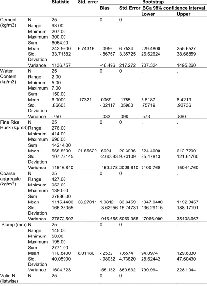
Table 2 shows the descriptive statistical analysis which was used to portray information in the data. It analysis the data statistically, reveals and details the information in the data. It also emphasis the data mean, median, sum, range, variance standard deviations, confidence level, residual errors in the data and the standard error in the data.

Table 1. Variables of results from hot moist zones (Awka) [9]

Level of factors and test

X1 = C cement kg/m3

X2= w water content kg/m3

X3 = Fa fine rice husk kg/m3

X4 = Ca coarse Aggregate kg/m0

Slump Swet (mm)

Xnar Highest level (+) Xim Lowest level (-) Xer Central Level (0) average

Interval of Change Δ 300 207 254

46

7 5 6

1

690 414 552

138

1380 953 1167

213

Test No X1 X2 X3 X4 Y1

1 207 5 414 953 88

2 207 7 690 953 109

3 207 5 690 953 160

4 207 5 690 953 156

5 300 7 414 953 65

6 300 5 690 1380 81

7 207 7 690 1380 99

8 207 7 690 1380 50

9 207 6 552 1167 67

10 300 7 552 1167 62

11 254 5 552 1167 82

12 254 7 552 1167 93

13 254 6 414 953 166

14 300 5 690 953 157

15 207 7 414 1380 110

16 254 6 552 1167 179

17 207 5 414 953 105

18 207 5 690 953 101

19 254 7 552 1167 95

20 254 5 552 1167 90

21 254 7 690 953 89

22 254 6 414 1167 102

23 254 6 552 1380 105

24 254 6 552 953 195

25 254 6 552 1167 165

(4)

Table 2. Descriptive statistics analysis

Statistic Std. error Bootstrap

Bias Std. Error BCa 98% confidence interval Lower Upper

Cement (kg/m3)

N 25 0 0 . .

Range 93.00

Minimum 207.00 Maximum 300.00

Sum 6064.00

Mean 242.5600 6.74316 -.0956 6.7534 229.4800 255.6527

Std. Deviation

33.71582 -.86767 3.35725 26.62624 38.66859

Variance 1136.757 -46.496 217.272 707.324 1495.260

Water Content (kg/m3)

N 25 0 0 . .

Range 2.00

Sum 150.00

Mean 6.0000 .17321 .0069 .1755 5.6187 6.4213

Std. Deviation

.86603 -.02117 .05960 .75719 .92736

Variance .750 -.033 .098 .573 .860

Fine Rice Husk(kg/m3)

N 25 0 0 . .

Range 276.00

Sum 14214.00

Mean 568.5600 21.55629 .6624 20.3936 524.4000 612.7200

Std. Deviation

107.78145 -2.60083 9.73109 85.47813 121.61760

Variance 11616.840 -459.278 2026.610 7109.760 15044.760

Coarse aggregate (kg/m3)

N 25 0 0 . .

Range 427.00

Sum 27886.00

Mean 1115.4400 33.27011 1.9812 33.3459 1047.0400 1192.3457

Std. Deviation

166.35055 -3.62956 15.74731 136.29115 188.17191

Variance 27672.507 -946.655 5066.358 17966.090 35408.667

Slump (mm) N 25 0 0 . .

Range 145.00

Sum 2771.00

Mean 110.8400 8.01180 -.2532 7.6574 94.0974 129.6330

Std. Deviation

40.05900 -.98032 4.73820 28.62442 47.60430

Variance 1604.723 -55.152 360.532 799.994 2281.044

Valid N (listwise)

(5)

Coarse Aggregate (kg/m3)

Table 3. Case processing summary

Coarse aggregate (kg/m3)

Cases

Valid Missing Total

N Percent N Percent N Percent

Slump (mm)

953.00 11 100.0% 0 0.0% 11 100.0%

1167.00 9 100.0% 0 0.0% 9 100.0%

1380.00 5 100.0% 0 0.0% 5 100.0%

Table 4. Coarse aggregate M-Estimators

Coarse aggregate (kg/m3) Statistic Bootstrap

Bias Std. error BCa 98% confidence interval Lower Upper

Slump (mm)

953.00

Huber's M-Estimator 125.6317 -.3535i 19.0402i 89.7525i 160.2611i Tukey's Biweight 125.8833 -1.5816i 22.1158i 88.4845i 162.9755i Hampel's M-Estimator 126.4545 -.7262i 19.6975i 88.8551i 162.6822i

Andrews' Wave 125.8787 -1.6135i 22.1574i 88.4890i 162.9655i

1167.00

Huber's M-Estimator 92.4295 2.4849j 14.4906j 67.4795j 162.6503j

Tukey's Biweight 86.0199 6.2427j 16.8065j .j .j

Hampel's M-Estimator 86.0148 7.9399j 15.8676j .j .j

Andrews' Wave 86.0156 6.2076j 16.8339j .j .j

1380.00

Huber's M-Estimator 95.0578 -.9595k 10.1189k 65.6282k 107.5000k

Tukey's Biweight 99.4180 -3.5515k 10.9710k 68.4169k 108.4724k

Hampel's M-Estimator 94.6979 -.1041k 10.6841k 65.5000k 108.7500k

Andrews' Wave 99.6441 -3.7565k 10.9742k 68.4245k 108.4839k

Table 5. Tests of normality

Coarse aggregate (kg/m3) Kolmogorov-Smirnov Shapiro-Wilk Statistic df Sig. Statistic df Sig.

Slump (mm) 953.00 .216 11 .160 .924 11 .351

1167.00 .296 9 .022 .826 9 .041

1380.00 .259 5 .200* .876 5 .290

Fine Rice Husk (kg/m3)

Table 6. Fine M-Estimators

Fine (kg/m3) Statistic Bootstrap

Bias Std. Error BCa 98% confidence interval Lower Upper

Slump (mm)

414.00

Huber's M-Estimator 101.3111 1.4796i 10.8098i 77.7682i 135.5000i

Tukey's Biweight 98.4511 3.1955i 11.4013i .i .i

Hampel's M-Estimator 98.8138 3.7421i 10.9845i .i .i

Andrews' Wave 98.4261 3.1892i 11.4333i .i .i

552.00

Huber's M-Estimator 98.0502 5.0902j 19.8758j 69.5201j 174.0098j

Tukey's Biweight 86.0940 13.3154j 23.0046j .j .j

Hampel's M-Estimator 96.8503 5.8041j 21.1481j 66.8653j 175.2135j

Andrews' Wave 85.7565 13.5551j 23.0681j .j .j

690.00

Huber's M-Estimator 106.3838 4.4396k 19.3970k 81.0441k 156.4626k

Tukey's Biweight 107.4876 2.2151k 21.0520k 84.2190k 157.9911k

Hampel's M-Estimator 109.2851 1.6786k 20.2975k 85.0286k 158.0000k

(6)

Fine (kg/m3) Kolmogorov-Smirnov Shapiro-Wilk Statistic df Sig. Statistic df Sig.

Slump (mm)

414.00 .286 6 .137 .904 6 .396

552.00 .269 10 .039 .850 10 .057

690.00 .210 9 .200* .903 9 .269

Water Content (kg/m3)

Water content (kg/m3)

Cases

Valid Missing Total

N Percent N Percent N Percent

Slump (mm)

5.00 9 100.0% 0 0.0% 9 100.0%

6.00 7 100.0% 0 0.0% 7 100.0%

7.00 9 100.0% 0 0.0% 9 100.0%

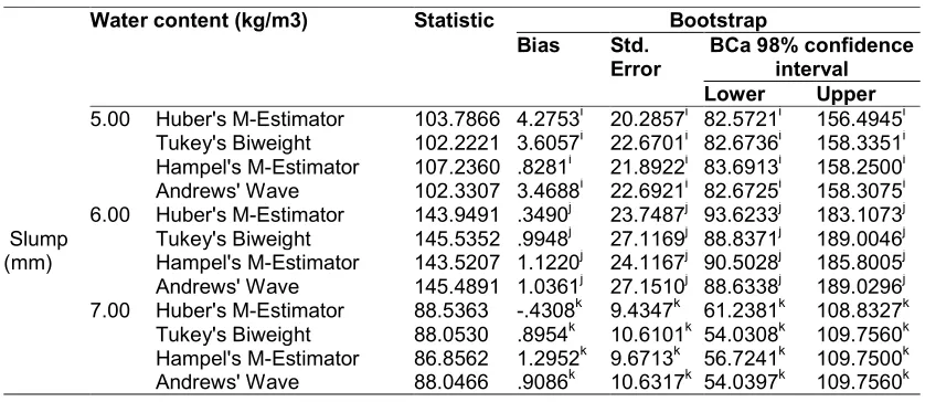
Table 9. Water content (kg/m3) M-Estimators

Water content (kg/m3) Statistic Bootstrap Bias Std.

Error

BCa 98% confidence interval Lower Upper

Slump (mm)

5.00 Huber's M-Estimator 103.7866 4.2753i 20.2857i 82.5721i 156.4945i Tukey's Biweight 102.2221 3.6057i 22.6701i 82.6736i 158.3351i Hampel's M-Estimator 107.2360 .8281i 21.8922i 83.6913i 158.2500i

Andrews' Wave 102.3307 3.4688i 22.6921i 82.6725i 158.3075i

6.00 Huber's M-Estimator 143.9491 .3490j 23.7487j 93.6233j 183.1073j Tukey's Biweight 145.5352 .9948j 27.1169j 88.8371j 189.0046j Hampel's M-Estimator 143.5207 1.1220j 24.1167j 90.5028j 185.8005j

Andrews' Wave 145.4891 1.0361j 27.1510j 88.6338j 189.0296j

7.00 Huber's M-Estimator 88.5363 -.4308k 9.4347k 61.2381k 108.8327k

Tukey's Biweight 88.0530 .8954k 10.6101k 54.0308k 109.7560k

Hampel's M-Estimator 86.8562 1.2952k 9.6713k 56.7241k 109.7500k

Andrews' Wave 88.0466 .9086k 10.6317k 54.0397k 109.7560k

Water Content (kg/m3) Kolmogorov-Smirnov Shapiro-Wilk Statistic df Sig. Statistic df Sig.

Slump (mm) 5.00 .263 9 .073 .787 9 .014

6.00 .271 7 .129 .901 7 .338

7.00 .226 9 .200* .899 9 .246

Cement (kg/m3)

Cement (kg/m3)

Cases

Valid Missing Total N Percent N Percent N Percent

Slump (mm) 207.00 10 100.0% 0 0.0% 10 100.0%

254.00 11 100.0% 0 0.0% 11 100.0%

(7)

Tables 3, 8 and 11 reveal the validity of a data and the missing values in the data using a method that is known as case processing summary. This method reveals the number of values in the lower boundary, mean boundary and upper boundary in the data system and the possibility of valid data in the boundaries. However, it also reveals the possible missing data in the lower boundary, mean boundary and upper boundary in the data system.

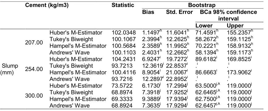
Tables 4, 6, 9 and 12 shows that some M Estimators cannot be computed in one or more split files because of the highly centralized distribution around the median. Some results could not be computed from jackknife samples or

Table 12

Cement (kg/m3)

Slump (mm)

207.00

Huber's M-Estimator Tukey's Biweight Hampel's M-Estimator Andrews' Wave

254.00

300.00

Generalized

Tables 3, 8 and 11 reveal the validity of a data and the missing values in the data using a method that is known as case processing summary. This method reveals the number of mean boundary and upper boundary in the data system and the possibility of valid data in the boundaries. However, it also reveals the possible missing data in the lower boundary, mean boundary and upper boundary in the data system.

shows that some M-Estimators cannot be computed in one or more split files because of the highly centralized distribution around the median. Some results could not be computed from jackknife samples or

the estimators, so this confidence interval is computed by the percentile method rather than the BCa method. M-Estimators is a method used to determine the average estimated confidence level of the data using several estimation methods to achieve more effective results. The estimation methods developed their

methods around the lower value, mean value and the upper value of the used data. However, it will be noted that the estimated confidence level in this research is 98 percent (%), this is used because of the economic importance and its necessity to construction. The superscript of I, j k and h express the concrete mix component variations using different selected estimators.

Table 12. Cement (kg/m3) M-Estimators

Statistic Bootstrap

Bias Std. Error BCa 98% confidence interval Lower Upper

Estimator 102.0348 1.1497h 11.6041h 71.4591h 155.2357 100.1067 2.3994h 12.2625h 58.2672h 159.1125 Estimator 100.5684 2.3589h 11.9952h 70.2221h 158.9132 100.1103 2.4031h 12.2662h 58.1394h 159.1173 Estimator 104.2431 6.9247i 19.7272i 89.6182i 169.8525

93.7213 12.3619i 22.8537i .i .

Estimator 100.4116 8.9054i 21.0067i 86.6663i 173.9062

93.7216 12.2897i 22.8952i .i .

Estimator 73.5722 6.1730j 17.2994j 63.5000j,k 119.0000 68.8974 7.3918j 17.9252j 62.6465j,k 119.0000 Estimator 69.3333 9.3889j 17.9394j 62.7500j,k 119.0000 68.8924 7.3635j 17.9294j 62.6457j,k 119.0000

Generalized linear mixed models

the estimators, so this confidence interval is d by the percentile method rather than Estimators is a method used to determine the average estimated confidence level of the data using several estimation methods to achieve more effective results. The estimation methods developed their confidence methods around the lower value, mean value and the upper value of the used data. However, it will be noted that the estimated confidence level in this research is 98 percent (%), this is

used because of the economic importance and its necessity to construction. The superscript

of I, j k and h express the concrete mix component variations using different selected

confidence interval

Upper

155.2357h 159.1125h 158.9132h 159.1173h 169.8525i .i

173.9062i .i

(8)

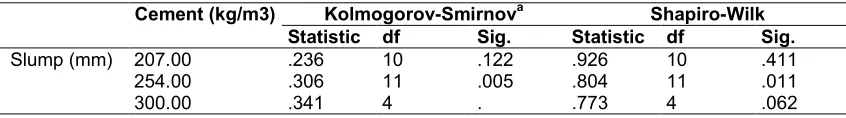
Table 13. Tests of normalityc

Cement (kg/m3) Kolmogorov-Smirnova Shapiro-Wilk Statistic df Sig. Statistic df Sig.

Slump (mm) 207.00 .236 10 .122 .926 10 .411

254.00 .306 11 .005 .804 11 .011

300.00 .341 4 . .773 4 .062

Tables 5, 7, 10 and 13 investigates and reveals tests of normality using Kolmogorov-Smirnov and Shapiro-Wilk which shows that statistically, the data is not normally distributed along the upper and lower boundaries of the data mean except at the mean. The cement data is significance along the mean of slump data but is not significance at the upper and lower boundary of the slump wet data. This is applicable in the two normality test methods applied.

4. CONCLUSION

On the basis of the statistical analysis, the derived mathematical model for the slumps (workability) and strength of concrete in a hot humid zone as functions of quantity of cement, water-cement ratio and quantity of aggregates, it is possible to evaluate the composition of the concrete mix by varying the independent factors (variables) for various seasons. The rice ash husk used will improve and strengthen the concrete mixture of the component although it can decompose within a long period of time. The statistical results developed will help to understand the data and what the data portrays.

COMPETING INTERESTS

Authors have declared that no competing interests exist.

REFERENCES

1. Ezeokonkwo JU. Quality control in construction, project. Effective Building

Procurement and Delivery in Nigerian Construction Industry. Rex Charles and Patrick Ltd. Nimo Anambra State. 2002;85-101.

2. Edeh et al. Analysis of environmental risk factors affecting rice farming in Ebonyi State, South Eastern Nigeria; 2011. 3. Obiegbu ME. The professional builder.

Magazine Published by Nigerian Institute of Building; 2007.

4. Aman A. Assessment of the quality strength and variability of the construction materials. Nigerian Institute of Structural Engineers Conference. 2010;10-12. 5. Dhir RK, Green JW. Protection of concrete

processing. Paper presented at

International Conference held at the University of Dundes Scotland, UK; 1990. 6. Imaga. Theory and practice of production

management. Afritrade International Limited Publishers. 8/10 Broad Street 10th Floor Western House; 1994.

7. Heiseman. Concrete characteristics. Sweet Haven Publishers; 2007.

8. Ezeokonkwo JU. Assessment of quality control of concrete production works in

Nigeria. Publisher: LAP LAMBERT

Academic Publishing, Deutschland, Germany; 2015.

[ISBN: 9783659389306]

9. Ezeokonkwo J, Uche Ikechukwu F.

Factorial analysis of concrete production in hot and warm humid zones in South East Nigeria. Advances in Engineering & Scientific Research. 2015;1(1):1-16.

© 2019 Ezeokonkwo et al.; This is an Open Access article distributed under the terms of the Creative Commons Attribution License (http://creativecommons.org/licenses/by/4.0), which permits unrestricted use, distribution, and reproduction in any medium, provided the original work is properly cited.

Peer-review history: