The Constrained Dantzig Selector with Enhanced
Consistency
∗Yinfei Kong [email protected]
Department of Information Systems and Decision Sciences Mihaylo College of Business and Economics
California State University at Fullerton Fullerton, CA 92831, USA
Zemin Zheng [email protected]
Department of Statistics and Finance
University of Science and Technololgy of China Hefei, Anhui 230026, China
Jinchi Lv [email protected]
Data Sciences and Operations Department Marshall School of Business
University of Southern California Los Angeles, CA 90089, USA
Editor:Sara van de Geer
Abstract
The Dantzig selector has received popularity for many applications such as compressed sensing and sparse modeling, thanks to its computational efficiency as a linear program-ming problem and its nice sampling properties. Existing results show that it can recover sparse signals mimicking the accuracy of the ideal procedure, up to a logarithmic factor of the dimensionality. Such a factor has been shown to hold for many regularization meth-ods. An important question is whether this factor can be reduced to a logarithmic factor of the sample size in ultra-high dimensions under mild regularity conditions. To provide an affirmative answer, in this paper we suggest the constrained Dantzig selector, which has more flexible constraints and parameter space. We prove that the suggested method can achieve convergence rates within a logarithmic factor of the sample size of the oracle rates and improved sparsity, under a fairly weak assumption on the signal strength. Such improvement is significant in ultra-high dimensions. This method can be implemented effi-ciently through sequential linear programming. Numerical studies confirm that the sample size needed for a certain level of accuracy in these problems can be much reduced.
Keywords: Sparse Modeling, Compressed Sensing, Ultra-high Dimensionality, Dantzig Selector, Regularization Methods, Finite Sample
1. Introduction
Due to the advances of technologies, big data problems appear increasingly common in the domains of molecular biology, machine learning, and economics. It is appealing to design procedures that can provide a recovery of important signals, among a pool of potentially huge number of signals, to a desired level of accuracy. As a powerful tool for producing interpretable models, sparse modeling via regularization has gained popularity for analyzing large-scale data sets. A common feature of the theories for many regularization methods is that the rates of convergence under the prediction or estimation loss usually involve the logarithmic factor of the dimensionality logp; see, for example, Bickel et al. (2009), van de Geer et al. (2011), and Fan and Lv (2013), among many others. From the asymptotic point of view, such a factor may be negligible or insignificant when p is not too large. It can, however, become no longer negligible or even significant in finite samples with large dimensionality, particularly when a relatively small sample size is considered or preferred. In such cases, the recovered signals and sparse models may tend to be noisy. Another consequence of this effect is that many noise variables tend to appear together with recovered important ones (Cand`es et al., 2008). An important and interesting question is whether such a factor can be reduced, say, to a logarithmic factor of the sample size logn, from ultra-high dimensions under mild regularity conditions.
In high-dimensional variable selection, there is a fast growing literature for different kinds of regularization methods with well established rates of convergence under the estimation and prediction losses. For instance, Cand`es and Tao (2007) proposed theL1-regularization
approach of the Dantzig selector by relaxing the normal equation to allow for correlation between the residual vector and all the variables, which can recover sparse signals as accu-rately as the ideal procedure, knowing the true underlying sparse model, up to a logarithmic factor logp. Later, Bickel et al. (2009) showed that the popularly used Lasso estimator (Tib-shirani, 1996) exhibits similar behavior as the Dantzig selector with a logp factor in the oracle inequalities for the prediction risk and bounds on the estimation losses in general nonparametric regression models. Furthermore, it has been proved in Raskutti et al. (2011) that the minimax rates of convergence for estimating the true coefficient vector in the high-dimensional linear regression model involve a logarithmic factor logp in the L2-loss and
prediction loss, under some regularity conditions on the design matrix. Other work for desired properties such as the oracle property on the L1 and more general regularization
includes Fan and Li (2001), Fan and Peng (2004), Zou and Hastie (2005), Zou (2006), van de Geer (2008), Lv and Fan (2009), Antoniadis et al. (2010), St¨adler et al. (2010), Fan and Lv (2011), Negahban et al. (2012), Chen et al. (2013), and Fan and Tang (2013), among many others.
constrained on that event will give a factor logninstead of logpin the rates of convergence under various estimation and prediction losses. However, to obtain model selection consis-tency it usually requires a uniform signal strength condition that the minimum magnitude of nonzero coefficients is at least of order {s(logp)/n}1/2 ((Fan and Lv, 2013) and (Zheng
et al., 2014)), where s stands for the size of the low-dimensional parameter vector. We doubt the necessity of the model selection consistency and the uniform signal strength of order{s(logp)/n}1/2 for achieving the logarithmic factor lognin ultra-high dimensionality.
In this paper, we suggest the constrained Dantzig selector to study the rates of conver-gence with weaker signal strength assumption. The constrained Dantzig selector replaces the constant Dantzig constraint on correlations between the variables and the residual vector by a more flexible one, and considers a constrained parameter space distinguishing between zero parameters and significantly nonzero parameters. The main contributions of this paper are threefold. First, the convergence rates for the constrained Dantzig selector are shown to be within a factor of lognof the oracle rates instead of logp, a significant improvement in the case of ultra-high dimensionality and relatively small sample size. It is appealing that such an improvement is made with a fairly weak assumption on the signal strength without requiring model selection consistency. To the best of our knowledge, this assumption seems to be the weakest one in the literature of similar results; see, for example, Bickel et al. (2009) and Zheng et al. (2014). Two parallel theorems, under the uniform uncertainty principle condition and the restricted eigenvalue assumption, are established on the properties of the constrained Dantzig selector for compressed sensing and sparse modeling, respectively. Second, compared to the Dantzig selector, theoretical results of this paper show that the number of falsely discovered signs of our new selector, with an explicit inverse relation-ship to the signal strength, is controlled as a possibly asymptotically vanishing fraction of the true model size. Third, an active-set based algorithm is introduced to implement the constrained Dantzig selector efficiently. An appealing feature of this algorithm is that its convergence can be checked easily.
The rest of the paper is organized as follows. In Section 2, we introduce the constrained Dantzig selector. We present its compressed sensing and sampling properties in Section 3. In Section 4, we discuss the implementation of the method and present several simulation and real data examples. We provide some discussions of our results and some possible ex-tensions of our method in Section 5. All technical details are relegated to the Appendix.
2. The Constrained Dantzig selector
To simplify the technical presentation, we adopt the model setting in Cand`es and Tao (2007) and present the main ideas focusing on the linear regression model
y=Xβ+ε, (1)
or light-tailed error distributions without much difficulty. See, for example, the technical analysis in Fan and Lv (2011) and Fan and Lv (2013).
In both problems of compressed sensing and sparse modeling, we are interested in recovering the support and nonzero components of the true regression coefficient vector
β0 = (β0,1, . . . , β0,p)T, which we assume to be sparse with s nonzero components, for the case when the dimensionality p may greatly exceed the sample size n. Throughout this paper, p is implicitly understood as max{n, p} and s ≤ min{n, p} to ensure model iden-tifiability. To align the scale of all covariates, we assume that each column of X, that is, each covariate vector xj, is rescaled to haveL2-norm n1/2, matching that of the constant
covariate vector1. The Dantzig selector (Cand`es and Tao, 2007) is defined as
b
βDS= argminβ∈
Rp kβk1 subject to kn
−1XT(y−Xβ)k
∞≤λ1, (2)
whereλ1 ≥0 is a regularization parameter. The above constant Dantzig selector constraint
on correlations between all covariates and the residual vector may not be flexible enough to differentiate important covariates and noise covariates. We introduce an extension of the Dantzig selector, the constrained Dantzig selector, defined as
b
βcds=argminβ∈B λ kβk1
subject to |n−1xTj(y−Xβ)| ≤λ01{|βj|≥λ}+λ11{|βj|=0} forj= 1, . . . , p,
(3)
where λ0 ≥ 0 is a regularization parameter and Bλ = {β ∈ Rp : βj = 0 or|βj| ≥
λfor each j} is the constrained parameter space for some λ≥ 0. When we choose λ= 0 and λ0 = λ1, the constrained Dantzig selector becomes the Dantzig selector.
Through-out this paper, we choose the regularization parameters λ0 and λ1 asc0{(logn)/n}1/2 and c1{(logp)/n}1/2, respectively, withλ0≤λ1as well asc0andc1two sufficiently large positive
constants, and assume that λis a parameter greater thanλ1. The two parametersλ0 and λ1differentially bound two types of correlations: on the support of the constrained Dantzig
selector, the correlations between covariates and residuals are bounded, up to a common scale, by λ0; on its complement, however, the correlations are bounded through λ1. In the
ultra-high dimensional case, meaning logp = O(nα) for some 0 < α < 1, the constraints involving λ0 are tighter than those involving λ1, in which λ1 is a universal regularization
parameter for the Dantzig selector; see Cand`es and Tao (2007) and Bickel et al. (2009). We now provide more insights into the new constraints in the constrained Dantzig se-lector. First, it is worthwhile to notice that if β0 ∈ Bλ, β0 can satisfy new constraints
The threshold λ inBλ distinguishes between important covariates with strong effects and noise covariates with weak effects. As shown in Fan and Lv (2013), this feature can lead to improved sparsity and effectively prevent overfitting by making it harder for noise covariates to enter the model.
3. Main results
In this section, two parallel theoretical results are introduced based on the uniform uncer-tainty principle (UUP) condition and restricted eigenvalue assumption, respectively. Al-though the UUP condition may be relatively stringent in some applications, we still present one theorem for our method under this condition in Section 3.1 for the purpose of compar-ison with the original Dantzig selector.
3.1 Nonasymptotic compressed sensing properties
Since the Dantzig selector was introduced partly for applications in compressed sensing, we first study the nonasymptotic compressed sensing properties of the constrained Dantzig selector by adopting the theoretical framework in Cand`es and Tao (2007). They introduced the uniform uncertainty principle condition defined as follows. Denote byXT a submatrix of X consisting of columns with indices in a setT ⊂ {1, . . . , p}. For the true model size s, define thes-restricted isometry constant of X as the smallest constantδs such that
(1−δs)khk22≤n−1kXThk22 ≤(1 +δs)khk22
for any set T with size at mosts and any vectorh. This condition requires that each sub-matrix of Xwith at mostscolumns behaves similarly as an orthonormal system. Another constant, the s-restricted orthogonality constant, is defined as the smallest quantity θs,2s such that
n−1|hXTh,XT0h0i| ≤θs,2skhk2kh0k2
for all pairs of disjoint sets T, T0 ⊂ {1, . . . , p} with |T| ≤ sand |T0| ≤ 2s and any vectors
h,h0. The uniform uncertainty principle condition is simply stated as
δs+θs,2s<1. (4) For notational simplicity, we drop the subscripts and denote these two constants by δ and
θ, respectively. Without loss of generality, assume that supp(β0) = {1 ≤ j ≤ p : β0,j 6= 0}={1, . . . , s}hereafter. To evaluate the sparse recovery accuracy, we consider the number of falsely discovered signs defined as FS(βb) =|{j = 1, . . . , p: sgn(βbj) 6= sgn(β0,j)}| for an
estimator βb = (βb1, . . . ,βbp)T. Now we are ready to present the nonasymptotic compressed
sensing properties of the constrained Dantzig selector.
1−O(n−c) for c= (c20∧c21)/(2σ2)−1, the constrained Dantzig selector βb satisfies that
kβb−β0k1 ≤2
√
5(1−δ−θ)−1c0s
p
(logn)/n,
kβb−β0k2 ≤
√
5(1−δ−θ)−1c0
p
s(logn)/n,
FS(βb)≤Cc21s(logp)/(nλ2).
If in addition λ > √5(1−δ−θ)−1c0
p
s(logn)/n, then with the same probability, it also holds thatsgn(βb) = sgn(β0)and kβb−β0k∞≤2c0k(n−1XT1X1)−1k∞
p
(logn)/n, where X1 is an n×ssubmatrix of X corresponding to s nonzero β0,j’s.
The constant c in the above probability bound can be sufficiently large since both constantsc0 andc1 are assumed to be large, while the constantCcomes from Theorem 1.1
in Cand`es and Tao (2007); see the proof in the Appendix for details. In the above bound on the L∞-estimation loss, it holds that k(n−1XT1X1)−1k∞ ≤ s1/2k(n−1XT1X1)−1k2 ≤
(1−δ)−1s1/2. See Section 3.2 for more discussion on this quantity.
From Theorem 1, we see improvements of the constrained Dantzig selector over the Dantzig selector, which has a convergence rate, in terms of theL2-estimation loss, up to a
factor logp of that for the ideal procedure. However, the sparsity property of the Dantzig selector was not investigated in Cand`es and Tao (2007). In contrast, the constrained Dantzig selector is shown to have an inverse quadratic relationship between the number of falsely discovered signs and the threshold λ, revealing that its model selection accuracy increases with the signal strength. The number of falsely discovered signs can be controlled below or as an asymptotically vanishing fraction of the true model size, since FS(βb)≤Cs(λ1/λ)2≤
(1 +λ1/λ)−2s < s by assuming λ > C1/2(1 +λ1/λ0)λ1.
Another advantage of the constrained Dantzig selector lies in its convergence rates. In the case of ultra-high dimensionality which is typical in compressed sensing applications, its prediction and estimation losses can be reduced from the logarithmic factor logp to logn
with overwhelming probability. In particular, only a fairly weak assumption on the signal strength is imposed to attain such improved convergence rates. In fact, it has been shown in Raskutti et al. (2011) that without any condition on the signal strength, the minimax convergence rate ofL2 risk has an upper bound of orderO{s1/2(logp)/n}. Especially, they
claimed that the Dantzig selector can achieve such minimax rate, but requires a relatively stronger condition on the design matrix than nonconvex optimization algorithms to deter-mine the minimax upper bounds. We push a step forward that the constrained Dantzig selector, with additional signal strength conditions, can attain the L2-estimation loss of a
smaller order than O{s1/2(logp)/n} in ultra-high dimensions.
There exist other methods which have been shown to enjoy convergence rates of the same order as well, for example, in Zheng et al. (2014) for high-dimensional thresholded regression. However, these results usually rely on a stronger condition on signal strength, such as, the minimum signal strength is at least of order{s(logp)/n}1/2. In another work,
Fan and Lv (2011) showed that the nonconcave penalized estimator can have a consistency rate of Op(s1/2n−γlogn) for some γ ∈(0,1/2] under the L2-estimation loss, which can be
a smaller number of observations will be needed for the constrained Dantzig selector to attain the same level of accuracy in compressed sensing, as the Dantzig selector, which is demonstrated in Section 4.2.
3.2 Sampling properties
The properties of the Dantzig selector have also been extensively investigated in Bickel et al. (2009). They introduced the restricted eigenvalue assumption with which the oracle inequalities under various prediction and estimation losses were derived. We adopt their theoretical framework and study the sampling properties of the constrained Dantzig selector under the restricted eigenvalue assumption stated below. A positive integermis said to be in the same order ofsifm/scan be bounded from both above and below by some positive constants.
Condition 1 For some positive integermin the same order ofs, there exists some positive constant κ such that kn−1/2Xδk
2 ≥κmax{kδ1k2,kδ01k2} for all δ∈Rp satisfying kδ2k1 ≤ kδ1k1, where δ = (δT1,δT2)T, δ1 is a subvector of δ consisting of the first s components, and δ01 is a subvector of δ2 consisting of the max{m, Cms(λ1/λ)2} largest components in magnitude, with Cm some positive constant.
Condition 1 is a basic assumption on the design matrix X for deriving the oracle in-equalities of the Dantzig selector. Since we assume that supp(β0) = {1, . . . , s}, Condition 1 indeed plays the same role as the restricted eigenvalue assumption RE(s, m,1) in Bickel et al. (2009), which assumes the inequality in Condition 1 holds for any subset with size no larger thansto cover all possibilities of supp(β0). See (10) in the Appendix for insights into the basic inequalitykδ2k1≤ kδ1k1 and Bickel et al. (2009) for more detailed discussions on
this assumption.
Theorem 2 Assume that Condition 1 holds and β0 ∈ Bλ with λ ≥ Cm1/2(1 +λ1/λ0)λ1. Then the constrained Dantzig selector βb satisfies with the same probability as in Theorem
1 that
n−1/2kX(βb−β0)k2=O(κ−1 p
s(logn)/n), kβb−β0k1 =O(κ−2s p
(logn)/n),
kβb−β0k2=O(κ−2 p
s(logn)/n), FS(βb)≤Cmc21s(logp)/(nλ2).
If in addition λ > 2√5κ−2c0s1/2
p
(logn)/n, then with the same probability it also holds thatsgn(βb) = sgn(β0) and kβb−β0k∞=O{k(n−1XT1X1)−1k∞
p
(logn)/n}.
Theorem 2 establishes asymptotic results on the sparsity and oracle inequalities for the constrained Dantzig selector under the restricted eigenvalue assumption. This assumption, which is an alternative to the uniform uncertainty principle condition, has also been widely employed in high-dimensional settings. In Bickel et al. (2009), an approximate equivalence of the Lasso estimator (Tibshirani, 1996) and Dantzig selector was proved under this as-sumption, and the Lasso estimator was shown to be sparse with sizeO(φmaxs), whereφmax
of falsely discovered signs FS(βb)≤Cms(λ1/λ)2=o(s) whenλ1 =o(λ). Similar as in
Theo-rem 1, the constrained Dantzig selector improves over both Lasso and the Dantzig selector in terms of convergence rates, a reduction of the logpfactor to logn.
Let us now take a closer look at the relationship between the faster rates of convergence and the assumptions on the signal strength and sparsity. Observe that the enhanced consis-tency results require the minimum signal strength to be at least of order (logp)/√nlogn, in view of the assumption λ ≥ Cm1/2(1 +λ1/λ0)λ1. Assume for simplicity that kβ0k2 is
bounded away from both zero and ∞. Then the order of the minimum signal strength yields an upper bound on the sparsity levels=O{n(logn)/(logp)2}, which means that the
sparsitysis required to be smaller when the dimensionality pbecomes larger. In the ultra-high dimensional setting of logp=O(nα) with 0< α <1, we then haves=O(n1−2αlogn). Thus the classical convergence rates involving s(logp)/n = O(n−αlogn) still go to zero asymptotically, while the rates established in our paper are improved with s(logp)/n re-placed bys(logn)/n=O{n−2α(logn)2}. We see a gain on the convergence rate of a factor
nα/(logn) at the cost of the aforementioned signal strength and sparsity assumptions. One can see that results in Theorems 1 and 2 are approximately equivalent, while the latter presents an additional oracle inequality on the prediction loss. An interesting phenomenon is that if adopting a simpler version, that is, the Dantzig selector equipped with the thresholding constraint only, we can also obtain similar results as in Theorems 1 and 2, but with a stronger condition on signal strength such as λ s1/2λ1. In this
sense, the constrained Dantzig selector is also an extension of the Dantzig selector equipped with the thresholding constraint only, but enjoys better properties. Some comprehensive results on the prediction and variable selection properties have also been established in Fan and Lv (2013) for various regularization methods, revealing their asymptotic equivalence in the thresholded parameter space. However, as mentioned in Section 3.1, improved rates as in Theorem 2 commonly require a stronger assumption on the signal strength, which is
β0 ∈ Bλ withλs1/2λ1; see, for example, Theorem 2 of Fan and Lv (2013).
For the quantity k(n−1XT1X1)−1k∞ in the above bound on the L∞-estimation loss, if
X1 takes the form of a common correlation matrix (1−ρ)Is+ρ1s1Ts for some ρ∈[0,1), it is easy to check that k(n−1XT1X1)−1k∞= (1−ρ)−1{1 + (2s−3)ρ}/{1 + (s−1)ρ}, which is bounded regardless of the value of s.
3.3 Asymptotic properties of computable solutions
The nonasymptotic and sampling properties of the constrained Dantzig selector, as the global minimizer, have been established in Sections 3.1 and 3.2, respectively. However, it is not guaranteed that the global minimizer can be generated by a computational algorithm. Moreover, a computable solution, generated by any algorithm, may only be a local minimizer in many cases. Under certain regularity conditions, we demonstrate that the local minimizer of our method can still share the same nice asymptotic properties as the global one.
Theorem 3 Let βb be a computable local minimizer of (3). Assume that there exist some
positive constantsc2,κ0 and sufficiently large positive constantc3 such thatkβbk0 ≤c2sand
minkδk
2=1,kδk0≤c3sn
−1/2kXδk
2 ≥κ0. Then under conditions of Theorem 2, βb enjoys the
In Section 4.1, we introduce an efficient algorithm that gives us a local minimizer. The-orem 3 indicates that the obtained solution can also enjoy the asymptotic properties in Theorem 2 under the extra assumptions that βb is a sparse solution with the number of
nonzero components comparable with s and the design matrix X satisfies a sparse eigen-value condition. Similar results for the computable solution can be found in Fan and Lv (2013, 2014), where the local minimizer is additionally assumed to satisfy certain constraint on the correlation between the residual vector and all the covariates.
4. Numerical studies
In this section, we first introduce an algorithm which can efficiently implement the con-strained Dantzig selector. Then several simulation studies and two real data examples are presented to evaluate the performance of our method.
4.1 Implementation
The constrained Dantzig selector defined in (3) depends on tuning parametersλ0,λ1, andλ.
We suggest some fixed values for λ0 and λto simplify the computation, since the proposed
method is generally not that sensitive to λ0 and λ as long as they fall in certain ranges.
In simulation studies to be presented, a value around {(logp)/n}1/2 for λ and a smaller
value for λ0, say 0.05{(logp)/n}1/2 or 0.1{(logp)/n}1/2, can provide us nice prediction and
estimation results. The value of λ0 is chosen to be smaller than {(logp)/n}1/2 to mitigate
the selection of noise variables and facilitate sparse modeling. The performance of our method with respect to different values of λ0 and λ is shown in simulation Example 2
in Section 4.2, which is a typical example that illustrates the robustness of the proposed method with respect to λ0 and λ.
For fixed λ0 and λ, we exploit the idea of sequential linear programming to produce
the solution path of the constrained Dantzig selector asλ1 varies. Choose a grid of values
for the tuning parameter λ1 in decreasing order with the first one being kn−1XTyk∞. It is easy to check that β = 0 satisfies all the constraints in (3) for λ1 = kn−1XTyk∞, and thus the solution isβb
cds=0 in this case. For eachλ1 in the grid, we use the solution from the previous one in the grid as an initial value to speed up the convergence. For a given
λ1, we define an active set, iteratively update this set, and solve the constrained Dantzig
selector problem. We name this algorithm as the CDS algorithm which is detailed in four steps below.
1. For a fixed λ1 in the grid, denote by βb
(0)
λ1 the initial value. Let βb
(0)
λ1 be zero when
λ1 =kn−1XTyk∞, and the estimate from previousλ1 in the grid otherwise.
2. Denote by βb
(k)
λ1 the estimate from the kth iteration. Define the active set A as the support ofβb
(k)
λ1 and A
cits complement. Let b be a vector with constant components
A. Solve the following linear program on the new set A:
b
βA= argmin kβAk1 subject to |n−1XTA(y−XAβA)| bA, (5) where is understood as componentwise no larger than and the subscript A also indicates a submatrix with columns corresponding toA. For the solution obtained in (5), set all its components smaller than λin magnitude to zero.
3. Update the active setAas the support ofβbA. Solve the Dantzig selector problem on
this active set withλ0 as the regularization parameter:
b
βA= argmin kβAk1 subject to kn−1XAT(y−XAβA)k∞≤λ0. (6)
Letβb
(k+1)
A =βbA and βb
(k+1)
Ac =0, which give the solution for the (k+ 1)th iteration.
4. Repeat steps 2 and 3 until convergence for a fixed λ1 and record the estimate from
the last iteration as βbλ
1. Jump to the next λ1 if βbλ1 ∈ Bλ, and stop the algorithm otherwise.
With the solution path produced, we use the cross-validation to select the tuning pa-rameterλ1. One can also tuneλ0 and λsimilarly as forλ1, but as suggested before, some
fixed values for them suffice to obtain satisfactory results.
The rationales of the constrained Dantzig selector algorithm are as follows. Step 1 defines the initial value (0th iteration) for each λ1 in the grid. In step 2, starting with a
smaller active set, we add variables that violate the constrained Dantzig selector constraints to eliminate such conflict. As a consequence, some components of bA are of value λ1
instead of λ0. Therefore, we need to further solve (6) in step 3 by noting that restricted on
its support, the constrained Dantzig selector should be a solution to the Dantzig selector problem with parameter λ0. An early stopping of the solution path is imposed in step 4 to
make this algorithm computationally more efficient.
An appealing feature of this algorithm is that its convergence can be checked easily. Once there are no more variables violating the constrained Dantzig selector constraints, that is, {j ∈ Ac : |n−1xT
j(y−XβbA)| > λ1} = ∅, the iteration stops and the algorithm
converges. In other words, the convergence of the algorithm is equivalent to that of the active set which can be checked directly. When the algorithm converges, the solution lies in the feasible set of the constrained Dantzig selector problem and is a global minimizer restricted on the active set, and is thus a local minimizer.
In simulation Example 2 of Section 4.2, we tracked the convergence property of the algorithm on 100 data sets forp= 1000, 5000, and 10000, respectively. In all cases, we ob-serve that the algorithm always converged over all 100 simulations, indicating considerable stability of this algorithm. Another advantage of the algorithm is that it is built upon the Dantzig selector in lower dimensions, so it inherits the computational efficiency.
4.2 Simulation studies
of the constrained Dantzig selector in comparison with the Dantzig selector, thresholded Dantzig selector, Lasso, elastic net (Zou and Hastie, 2005), and adaptive Lasso (Zou, 2006). Two simulation studies were considered, with the first one investigating sparse recovery for compressed sensing and the second one examining sparse modeling.
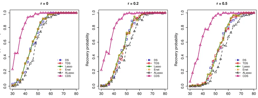
The setting of the first simulation example is similar to that of the sparse recov-ery example in Lv and Fan (2009). The noiseless sparse recovrecov-ery example is considered here since the Dantzig selector problem originated from compressed sensing. We want to evaluate the capability of our constrained Dantzig selector in recovering sparse signals as well. We generated 100 data sets from model (1) without noise, that is, the linear equa-tion y = Xβ0 with (s, p) = (7,1000). The nonzero components of β0 were set to be (1, −0.5, 0.7, −1.2, −0.9, 0.3, 0.55)T lying in the first seven components, andnwas cho-sen to be even integers between 30 and 80. The rows of the design matrix Xwere sampled as independent and identically distributed (i.i.d.) copies from N(0,Γr), with Γr a p×p matrix with diagonal elements being 1 and off-diagonal elements being r, and then each column was rescaled to have L2-norm
√
n. Three levels of population collinearity, r = 0, 0.2, and 0.5, were considered. Letλ0 and λbe in two small grids{0.001, 0.005, 0.01, 0.05,
0.1} and{0.05, 0.1, 0.15, 0.2}, respectively. We chose two grids of values for them since in the literature of compressed sensing, it is desirable to have the true support included among a set of estimates. The value 0.2 was chosen because it is close to{(logp)/n}1/2, which is
about {(log 1000)/80}1/2 in this example. Smaller values for λand λ
0 are also included in
the grid for conservativeness. We set the grid of values for λ1 as described in Section 4.1.
If any of the solutions in the path had exactly the same support as β0, it is counted as successful recovery. This criterion was applied to all other methods in this example for fair comparison.
Figure 1 presents the probabilities of exact recovery of sparseβ0based on 100 simulations by all methods. We see that all methods performed well in relatively large samples and had lower probability of successful sparse recovery when the sample size becomes smaller. The constrained Dantzig selector performed better than other methods over different sample sizes and three levels of population collinearity. In particular, the thresholded Dantzig selector performed similarly to the Dantzig selector, revealing that simple thresholding alone, instead of flexible constraints as in the constrained Dantzig selector, does not help much on signal recovery in this case.
The second simulation example adopts a similar setting to that in Zheng et al. (2014). We generated 100 data sets from the linear regression model (1) with Gaussian error
ε ∼ N(0, σ2In). The coefficient vector β0 = (vT, . . . ,vT,0T)T with the pattern v =
(βTstrong,βTweak)T repeated three times, where βstrong = (0.6,0,0,−0.6,0,0)T and βweak = (0.05,0,0,−0.05,0,0)T. The coefficient subvectors βstrong and βweak stand for the strong signals and weak signals in β0, respectively. The sample size and noise level were chosen as (n, σ) = (100,0.4), while the dimensionalityp was set to be 1000, 5000, and 10000. The rows of then×pdesign matrixXwere sampled as i.i.d. copies from a multivariate normal distribution N(0,Σ) with Σ = (0.5|i−j|)1≤i,j≤p. We applied all methods as in simulation example 1 and set λ0 = 0.01 and λ= 0.2 for our method. Similarly as before, the value of
0.2 was selected since it is close to {(log 1000)/100}1/2. The ideal procedure, which knows
30 40 50 60 70 80 0.0 0.2 0.4 0.6 0.8 1.0
r = 0
Reco ver y probability DS TDS Lasso Enet ALasso CDS
30 40 50 60 70 80
0.0 0.2 0.4 0.6 0.8 1.0
r = 0.2
Reco ver y probability DS TDS Lasso Enet ALasso CDS
30 40 50 60 70 80
0.0 0.2 0.4 0.6 0.8 1.0
r = 0.5
Reco ver y probability DS TDS Lasso Enet ALasso CDS
Figure 1: Probabilities of exact sparse recovery for the Dantzig selector (DS), thresholded Dantzig selector (TDS), Lasso, elastic net (Enet), adaptive Lasso (ALasso), and constrained Dantzig selector (CDS) in simulation example 1 of Section 4.2.
To compare these methods, we considered several performance measures: the prediction error, theLq-estimation loss withq = 1,2,∞, number of false positives, and number of false negatives for strong or weak signals. The prediction error is defined as E(Y −xTβb)2 with b
βan estimate and (xT, Y) an independent observation, and the expectation was calculated using an independent test sample of size 10000. A false positive means a falsely selected noise covariate in the model, while a false negative means a missed true covariate. Table 1 summarizes the comparison results by all methods. We observe that most weak covariates were missed by all methods. This is reasonable since the weak signals are around the noise level, making it difficult to distinguish them from the noise covariates. However, the constrained Dantzig selector outperformed other methods in terms of other prediction and estimation measures, and followed very closely the ideal procedure in all cases of p= 1000, 5000, and 10000. In particular, the L∞-estimation loss for the constrained Dantzig selector was similar to that for the oracle procedure, confirming tight bounds on this loss in Theorems 1 and 2. As the dimensionality grows higher, the constrained Dantzig selector performed similarly, while other methods suffered from high dimensionality. In particular, the thresholded Dantzig selector has been shown to improve over the Dantzig selector, but was still outperformed by the adaptive Lasso and constrained Dantzig selector in this example, revealing the necessity to introduce more flexible constraints instead of simple thresholding.
Recall that we have fixed λ0 = 0.01 and λ= 0.2 in the simulation example 2 across all
Table 1: Means and standard errors (in parentheses) of different performance measures by all methods in simulation example 2 of Section 4.2.
Measure DS TDS Lasso Enet ALasso CDS Oracle
p= 1000
PE (×10−2) 30.8 (0.6) 28.5 (0.5) 30.3 (0.5) 32.9 (0.7) 19.1 (0.1) 18.5 (0.1) 18.2 (0.1)
L1(×10−2) 201.9 (5.4) 137.2 (3.4) 186.1 (5.0) 211.1 (6.0) 58.0 (1.1) 51.3 (0.6) 41.5 (0.9)
L2(×10−2) 40.1 (0.7) 37.2 (0.7) 39.8 (0.7) 43.0 (0.8) 18.3 (0.3) 16.3 (0.2) 14.7 (0.3)
L∞ (×10−2) 19.0 (0.5) 18.6 (0.4) 19.3 (0.5) 20.7 (0.5) 9.1 (0.3) 7.5 (0.2) 8.4 (0.2) FP 44.4 (1.8) 5.5 (3.8) 36.3 (1.6) 44.1 (1.9) 0.5 (0.1) 0 (0) 0 (0) FN.strong 0 (0) 0 (0) 0 (0) 0 (0) 0 (0) 0 (0) 0 (0) FN.weak 5.3 (0.1) 5.9 (0.4) 5.4 (0.1) 5.3 (0.1) 6.0 (0.0) 6.0 (0.0) 0 (0)
p= 5000
PE (×10−2) 45.1 (1.1) 39.3 (1.1) 44.8 (1.1) 44.9 (1.1) 21.3 (0.6) 18.4 (0.1) 18.3 (0.1)
L1(×10−2) 289.3 (6.4) 184.6 (4.5) 270.8 (6.8) 273.2 (6.9) 71.2 (2.1) 50.4 (0.7) 41.7 (1.1)
L2(×10−2) 56.3 (1.1) 50.6 (1.1) 56.1 (1.1) 56.2 (1.1) 22.9 (0.9) 16.0 (0.2) 14.9 (0.4)
L∞ (×10−2) 27.4 (0.7) 25.1 (0.6) 27.8 (0.7) 27.8 (0.7) 12.7 (0.7) 7.3 (0.2) 8.8 (0.3) FP 60.6 (1.7) 7.0 (3.5) 53.5 (2.3) 53.8 (2.1) 1.0 (0.1) 0 (0) 0 (0) FN.strong 0 (0) 0 (0) 0 (0) 0 (0) 0 (0) 0 (0) 0 (0) FN.weak 5.2 (0.1) 6.0 (0.1) 5.4 (0.1) 5.3 (0.1) 5.9 (0.0) 6.0 (0.0) 0 (0)
p= 10000
PE (×10−2) 54.4 (16.2) 54.8 (17.4) 56.7 (23.1) 63.3 (21.7) 32.4 (32.3) 19.0 (0.5) 18.3 (0.1)
L1(×10−2) 322.3 (67.9) 218 (60.3) 296.3 (72.7) 334.8 (79.9) 86.6 (67.6) 51.9 (1.6) 41.3 (0.9)
L2(×10−2) 62.7 (14.1) 63.5 (14.9) 64.2 (17.7) 70.3 (16.8) 29.1 (26.3) 16.6 (0.6) 14.7 (0.3)
L∞ (×10−2) 30.5 (8.2) 32.5 (8.5) 31.8 (9.5) 34.4 (9.3) 15.8 (13.2) 7.8 (0.6) 8.5 (0.2) FP 69.9 (14.3) 6.9 (4.6) 56.89 (20.66) 64.06 (18.64) 0.78 (1.25) 0.01 (0.10) 0 (0) FN.strong 0 (0.1) 0 (0.1) 0.02 (0.14) 0.02 (0.14) 0.21 (0.95) 0.01 (0.10) 0 (0) FN.weak 6 (0.2) 6 (0.1) 5.98 (0.14) 5.97 (0.17) 6 (0) 6 (0) 0 (0)
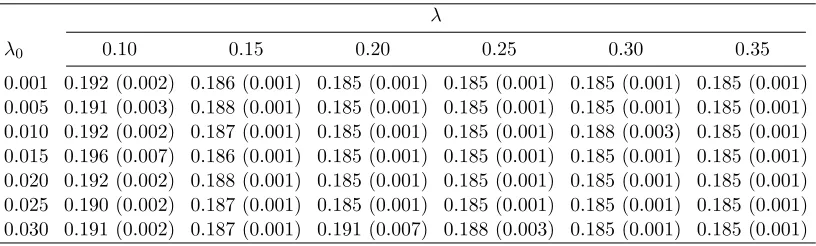
evaluate the robustness. The same performance measures were calculated. Here we only present the prediction error results to save space, and the other results are available upon request. The tuning parameter λ1 was chosen by cross-validation, similar as in Example
2. We can see from Table 2 that for all λ≥ 0.15 and all λ0 in the grids, the means and
standard errors of the prediction error are very close or even identical to those forλ0 = 0.01
and λ= 0.2. The prediction error in the case of λ= 0.1 is slightly higher since when the threshold becomes lower, some noise variables can be included. For the results on estimation losses as well as false positives and false negatives, we observe similar patterns confirming the robustness of our method with respect to the choices ofλ0 and λ.
4.3 Real data analyses
Table 2: Means and standard errors (in parentheses) of prediction error of the constrained Dantzig selector for different choices ofλ0 andλin simulation example 2 with p= 1000.
λ
λ0 0.10 0.15 0.20 0.25 0.30 0.35
0.001 0.192 (0.002) 0.186 (0.001) 0.185 (0.001) 0.185 (0.001) 0.185 (0.001) 0.185 (0.001) 0.005 0.191 (0.003) 0.188 (0.001) 0.185 (0.001) 0.185 (0.001) 0.185 (0.001) 0.185 (0.001) 0.010 0.192 (0.002) 0.187 (0.001) 0.185 (0.001) 0.185 (0.001) 0.188 (0.003) 0.185 (0.001) 0.015 0.196 (0.007) 0.186 (0.001) 0.185 (0.001) 0.185 (0.001) 0.185 (0.001) 0.185 (0.001) 0.020 0.192 (0.002) 0.188 (0.001) 0.185 (0.001) 0.185 (0.001) 0.185 (0.001) 0.185 (0.001) 0.025 0.190 (0.002) 0.187 (0.001) 0.185 (0.001) 0.185 (0.001) 0.185 (0.001) 0.185 (0.001) 0.030 0.191 (0.002) 0.187 (0.001) 0.191 (0.007) 0.188 (0.003) 0.185 (0.001) 0.185 (0.001)
The real PCR data set, originally studied in Lan et al. (2006), examines the genetics of two inbred mouse populations. This data set is comprised of n = 60 samples with 29 males and 31 females. Expression levels of 22,575 genes were measured. Following Song and Liang (2015), we study the linear relationship between the numbers of Phosphoenolpyruvate carboxykinase (PEPCK), a phenotype measured by quantitative real-time PCR, and the gene expression levels. Both the phenotype and predictors are continuous. As suggested in Song and Liang (2015), we only picked p = 2000 genes having the highest marginal correlations with PEPCK as predictors. The response was standardized to have zero mean and unit variance before we conducted the analysis. The 2000 predictors were standardized to have zero mean andL2-norm
√
nin each column. Then the data set was randomly split into a training set of 55 samples and a test set with the remaining 5 samples for 100 times. We setλ0 = 0.001 andλ= 0.02 in this real data analysis as well as the other one below for
conservativeness. Methods under comparison are the same as in the simulation studies.
Table 3 reports the means and standard errors of the prediction error on the test data as well as the median model size for each method. We see that the method CDS gave the lowest mean prediction error. Paired t-tests were conducted for the prediction errors of CDS versus DS, TDS, Lasso, ALasso, and Enet, respectively, to test the differences in performance across various methods. The corresponding p-values were 0.0243, 0.0014, 0.0081, 0.0001, and 0.0102, respectively, indicating significantly different prediction error from that for CDS.
Table 3: Means and standard errors of the prediction error and median model size over 100 random splits for the real PCR data set.
Method PE Model Size DS 0.773 (0.040) 54 TDS 0.897 (0.063) 14 Lasso 0.802 (0.043) 58 ALasso 0.922 (0.056) 5
Enet 0.793 (0.041) 58 CDS 0.660 (0.036) 21
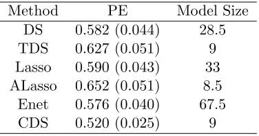
Similarly as in the analysis of the first real data set, we standardized the response and predictors beforehand. The training set contains 100 samples and was sampled randomly 100 times from the full data set. The remaining 20 samples at each time served as the test set. Results of prediction errors and median model sizes are presented in Table 4. It is clear that the proposed method CDS enjoys the lowest prediction error with a small model size. We conducted the same paired t-tests as in the real PCR data set for comparison. The corresponding p-values were 0.0351, 0.0058, 0.0164, 0.0004, and 0.0344, respectively, showing significant improvement.
Table 4: Means and standard errors of the prediction error and median model size over 100 random splits for the gene expression data set of rat eyes.
Method PE Model Size DS 0.582 (0.044) 28.5 TDS 0.627 (0.051) 9 Lasso 0.590 (0.043) 33 ALasso 0.652 (0.051) 8.5
Enet 0.576 (0.040) 67.5 CDS 0.520 (0.025) 9
5. Discussion
We have shown that the suggested constrained Dantzig selector can achieve convergence rates within a logarithmic factor of the sample size of the oracle rates in ultra-high dimen-sions under a fairly weak assumption on the signal strength. Our work provides a partial answer to an interesting question of whether convergence rates involving a logarithmic fac-tor of the dimensionality are optimal for regularization methods in ultra-high dimensions. It would be interesting to investigate such a phenomenon for more general regularization methods.
Our formulation of the constrained Dantzig selector uses the L1-norm of the
parameter to allow for different regularization on different covariates, as is in the adaptive Lasso (Zou, 2006). It would be interesting to investigate the behavior of these methods in more general model settings including generalized linear models and survival analysis. These problems are beyond the scope of the current paper and will be interesting topics for future research.
Appendix: Proofs of main results
Proof of Theorem 1
High probability event E. Recall that λ0 = c0
p
(logn)/n and λ1 = c1
p
(logp)/n. All the results in Theorems 1 and 2 will be shown to hold on a key event
E =kn−1XT1εk∞≤λ0 and kn−1XT2εk∞≤λ1 , (7)
where X1 is a submatrix of X consisting of columns corresponding to supp(β0) and X2
consists of the remaining columns. Thus we will have the same probability bound in both theorems. The probability bound on the event E in (7) can be easily calculated, using the classical Gaussian tail probability bound (see, for example, (Dudley, 1999)) and the Bonferroni inequality, as
pr(E)≥1−
pr(kn−1XT1εk∞> λ0) + pr(kn−1XT2εk∞> λ1)
= 1−
s(2/π)1/2σλ0−1n−1/2e−λ20n/(2σ2)+ (p−s)(2/π)1/2σλ−1
1 n
−1/2e−λ2 1n/(2σ2) = 1−Os n−c20/(2σ2)(logn)−1/2+ (p−s)p−c21/(2σ2)(logp)−1/2 , (8) where the last equality follows from the definitions ofλ0 andλ1. Letc= (c20∧c21)/(2σ2)−1
be a sufficiently large positive constant, since the two positive constantsc0andc1are chosen
large enough. Recall that p is understood implicitly as max{n, p} throughout the paper. Thus it follows from (8),s≤n, and n≤p that
pr(E) = 1−O n−c. (9)
From now on, we derive all the bounds on the event E. In particular, in light of (7) and
β0 ∈ Bλ it is easy to verify that conditional on E, the true regression coefficient vector β0
satisfies the constrained Dantzig selector constraints; in other words, β0 lies in the feasible set in (3).
Nonasymptotic properties of βb. We first make a simple observation on the
con-strained Dantzig selector βb = (βb1, . . . ,βbp)T. Recall that without loss of generality, we
assume supp(β0) = {1, . . . , s}. Let β0 = (βT1,0T)T with each component of β
1 being
nonzero, and βb = (βb
T
1,βb
T
2)T with βb1 a subvector of βb consisting of its first scomponents.
Denote by δ= (δT1,δ2T)T =βb−β0 the estimation error, whereδ1 =βb1−β1 and δ2 =βb2.
It follows from the global optimality of βb that kβb1k1+kβb2k1 = kβbk1 ≤ kβ0k1 = kβ1k1,
which entails that
We will see that this basic inequality kδ2k1 ≤ kδ1k1 plays a key role in the technical
derivations of both Theorem 1 and 2. Equipped with this inequality and conditional onE, we are now able to start the derivation of all results in Theorem 1 as follows.
The main idea is to first prove its sparsity property which will be presented in the next paragraph. Then, with the control on the number of false positives and false negatives, we derive an upper bound for the L2-estimation loss using the conclusion in Lemma 3.1 of
Cand`es and Tao (2007). Results on other types of losses follow accordingly.
(1) Sparsity. Recall that under the assumption of Theorem 1, β0 lies in its feasible set conditional on E. Since λ0 ≤λ1, by the definition of the constrained Dantzig selector, we
have |n−1XT(y−Xβb)| λ1, where is understood as componentwise no larger than.
Conditional on the eventE, substitutingybyXβ0+εand applying the triangle inequality yield
kn−1XTXδk∞≤2λ1. (11)
Furthermore, Lemma 3.1 in Cand`es and Tao (2007) still applies forδas long as the uniform uncertainty principle condition (4) holds. Together with (10) and (11), by applying the same argument as in the proof of Theorem 1.1 in Cand`es and Tao (2007), we obtain an
L2-estimation loss bound of kδk2 ≤ (Cs)1/2λ1 with C = 42/(1−δ−θ)2 some positive
constant.
Since both the true regression coefficient vector β0 and the constrained Dantzig selector
b
β lie in the constrained parameter space Bλ, the magnitude of any nonzero component in both β0 and βb is no smaller than λ. It follows that on the set of falsely discovered
signs, the component of δ = βb−β0 will be no smaller than λ. Then making use of the
obtained L2-estimation loss bound kδk2 ≤ (Cs)1/2λ1, it is immediate that the number of
falsely discovered signs is bounded from above by Cs(λ1/λ)2. Under the assumption of λ≥C1/2(1 +λ1/λ0)λ1, we have Cs(λ1/λ)2≤s(1 +λ1/λ0)−2 ≤s.
(2) L2-estimation loss. We further exploit the technical tool of Lemma 3.1 in Cand`es
and Tao (2007) to analyze the behavior of the estimation error δ = βb−β0. Let δ01 be a
subvector of δ2 consisting of the s largest components in magnitude, δ3 = (δT1,(δ
0
1)T)T,
and X3 a submatrix of X consisting of columns corresponding to δ3. We emphasize that
δ3 covers all nonzero components ofδsince the number of falsely discovered signs is upper
bounded bys, as showed in the previous paragraph. Therefore, kδ3kq=kδkq for all q >0. In view of the uniform uncertainty principle condition (4), an application of Lemma 3.1 in Cand`es and Tao (2007) results in
kδ3k2 ≤(1−δ)−1kn−1XT3Xδk2+θ(1−δ)−1s−1/2kδ2k1. (12)
On the other hand, from the basic inequality (10) it is easy to see that s−1/2kδ2k1 ≤ s−1/2kδ1k1 ≤ kδ3k2. Substituting it into (12) leads to
kδk2=kδ3k2 ≤(1−δ−θ)−1kn−1XT3Xδk2 (13)
Hence, to develop a bound for theL2-estimation loss it suffices to find an upper bound for kn−1XT3Xδk2.
Denote by A1, A2, and A3 the index sets of correctly selected variables, missed true
obtain from the definition of the constrained Dantzig selector along with its thresholding feature that|n−1XTA1(y−Xβb)| λ0,|n−1XTA
2(y−Xβb)| λ1, and|n
−1XT
A3(y−Xβb)| λ0.
Conditional on E, substitutingyby Xβ0+εand applying the triangle inequality give
kn−1XTA1Xδk∞≤2λ0 and kn−1XTA23Xδk∞≤λ0+λ1. (14) We now make use of the technical result on sparsity. SinceA23denotes the index set of false
positives and false negatives, its cardinality is also bounded by Cs(λ1/λ)2 with probability
at least 1−O(n−c). Therefore, by (14) we have
kn−1XT3Xδk22 ≤ kn−1XTA1Xδk22+kn−1XTA23Xδk22
≤skn−1XAT1Xδk2∞+Cs(λ1/λ)2kn−1XTA23Xδk
2
∞
≤4sλ20+Cs(λ1/λ)2(λ0+λ1)2.
Substituting this inequality into (13) yields
kδk2 ≤(1−δ−θ)−1
4sλ20+Cs(λ1/λ)2(λ0+λ1)2 1/2
.
Since we assumeλ≥C1/2(1+λ1/λ0)λ1, it follows thatC(λ1/λ)2(λ0+λ1)2≤λ20. Therefore,
we conclude that kδk2 ≤(1−δ−θ)−1(5sλ20)1/2.
(3) Other losses. Applying the basic inequality (10), we establish an upper bound for theL1-estimation loss
kδk1 =kδ1k1+kδ2k1 ≤2kδ1k1 ≤2s1/2kδ1k2 ≤2s1/2kδk2 ≤2(1−δ−θ)−1s(5λ20)1/2.
For the L∞-estimation loss, we additionally assume that λ > (1−δ −θ)−1(5sλ20) which can lead to the sign consistency, sgn(βb) = sgn(β0), in view of the L2-estimation loss
inequality above. Therefore, by the constrained Dantzig selector constraints we have
kn−1XT1(y −X1βb1)k∞ ≤ λ0 and thus kn−1XT1(ε−X1δ1)k∞ ≤ λ0. Then conditional
on E, it follows from the triangle inequality that kn−1XT1X1δ1k∞ ≤ 2λ0. Hence, kδk∞ =
kδ1k∞≤2k(n−1XT1X1)−1k∞λ0, which completes the proof.
Proof of Theorem 2
We continue to use the technical setup and notation introduced in the proof of Theorem 1. Results are parallel to those in Theorem 1 but presented in the asymptotic manner. The similarity lies in the rationale of the proof as well. The key element is to derive the sparsity and then construct an inequality for L2-estimation loss through the bridge n−1kXδk2
2. Inequalities for other types of losses are built upon this bound.
{1, . . . , s}, an application of similar arguments as in the proof of Theorem 7.1 in Bickel et al. (2009) yields the L2 oracle inequality kδk2 ≤ (Cms)1/2λ1 with Cm some positive constant dependent on m. Therefore, by the same arguments as in the proof of Theorem 1, it can be shown that the number of falsely discovered signs is bounded from above by
Cms(λ1/λ)2 and further by s(1 +λ1/λ0)−2 since λ≥Cm1/2(1 +λ1/λ0)λ1. Next we will go
through the proof of Theorem 7.1 in Bickel et al. (2009) in a more cautious manner and make some improvements in some steps with the aid of the obtained bound on the number of false positives and false negatives.
(2)L2-estimation loss. By Condition 1, we have a lower bound forn−1kXδk22. It is also
natural to derive an upper bound for it and build an inequality related to theL2-estimation
loss. It follows from (14) that
n−1kXδk22 ≤ kn−1XAT1Xδk∞kδA1k1+kn
−1XT
A23Xδk∞kδA23k1
≤2λ0kδA1k1+ (λ0+λ1)kδA23k1.
(15)
Since the cardinality of A23 is bounded by Cms(λ1/λ)2, applying the Cauchy-Schwarz
in-equality to (15) leads to n−1kXδk2
2 ≤ 2λ0kδA1k1+ (λ0 +λ1)kδA23k1 ≤ 2λ0s
1/2kδ
A1k2+
Cm1/2(λ0+λ1)s1/2λ1/λkδA23k2. This gives an upper bound for n
−1kXδk2
2. Combining this
with Condition 1 results in
2−1κ2(kδA1k
2
2+kδA23k
2
2)≤2λ0s1/2kδA1k2+C
1/2
m (λ0+λ1)s1/2λ1/λkδA23k2. (16)
Consider (16) in a two-dimensional space with respect to kδA1k2 and kδA23k2. Then the quadratic inequality (16) defines a circular area centered at (2κ−2λ0s1/2, κ−2Cm1/2(λ0 + λ1)s1/2λ1/λ). The term kδA1k
2
2 +kδA23k
2
2 is nothing but the squared distance between
the point in this circular area and the origin. One can easily identify the largest squared distance which is also the upper bound for the L2-estimation loss
kδk22=kδA1k
2
2+kδA23k
2 2 ≤4κ
−4
2λ0s1/2
2
+
Cm1/2(λ0+λ1)s1/2λ1/λ
2
.
With the assumption ofλ≥Cm1/2(1+λ1/λ0)λ1, we can show that
Cm1/2(λ0+λ1)s1/2λ1/λ 2≤ sλ20 and thuskδk2=O(κ−2s1/2λ0). This bound has significance improvement with the
fac-tor logp reduced to lognin the ultra-high dimensional setting.
(3) Other losses. With the L2 oracle inequality at hand, one can derive the L1 oracle
inequality kδk1 ≤s1/2kδk2 =O(κ−2sλ0) in a straightforward manner. For the prediction
loss, it follows from (15) that
n−1kXδk22 ≤2λ0s1/2kδA1k2+C
1/2
m (λ0+λ1)s1/2λ1/λkδA23k2.
Consider the problem of minimizing 2λ0s1/2kδA1k2+C
1/2
m (λ0+λ1)s1/2λ1/λkδA23k2 subject to (16). It is simply a two-dimensional linear optimization problem with a circular area as its feasible set. One can easily solve this minimization problem and obtain
n−1kXδk22≤2κ−2 2λ0s1/2
2
+Cm1/2(λ0+λ1)s1/2λ1/λ 2
Finally, for the L∞ oracle inequality, it follows from similar arguments as in the proof of Theorem 1 that kδk∞ ≤ 2k(n−1XT1X1)−1k∞λ0 = O{k(n−1X1TX1)−1k∞λ0}, which
con-cludes the proof.
Proof of Theorem 3
Denote by βbglobal the global minimizer of (3). Under the conditions of Theorem 2,
b
βglobal enjoys the same oracle inequalities and properties as in Theorem 2 conditional on
the event defined in (7). In particular, we have F S(βbglobal) =O(s). It follows that
kβbglobalk0≤ kβb0k0+F S(βbglobal) =O(s).
Letβb be a computable local minimizer of (3) produced by any algorithm satisfyingkβbk0≤
c2s. Denote by A= supp(βb)∪supp(βbglobal). Then we have
|A| ≤ kβbk0+kβbglobalk0=O(s)≤c3s
for some large enough positive constantc3.
We next analyze the difference between the two estimators, that is, δ =βb −βbglobal.
LetXA be a submatrix ofXconsisting of columns inA andδA a subvector ofδ consisting of components inA. SincekXT(y−Xβb)k∞=O(λ1) andkXT(y−Xβbglobal)k∞=O(λ1),
we can show that
kn−1XTAXAδAk2 ≤ |A|1/2kn−1XTAXAδAk∞=O(s1/2λ1).
By the assumption that minkδk
2=1,kδk0≤c3sn
−1/2kXδk
2 ≥κ0, the smallest singular value of n−1/2XAis bounded from below byκ0. Thus we havekδk2=kδAk2=O(s1/2λ1). Together
with the thresholding feature of the constrained Dantzig selector, it follows that the number of different indices between supp(βb) and supp(βbglobal) is bounded by O{s(λ1/λ)2}. This
sparsity property is essential for our proof and similar sparsity results can be found in Theorem 2.
Based on the aforementioned sparsity property and by the facts thatkXT
e
A1Xδk∞≤2λ0
and kXT
e
A23Xδk∞ ≤ λ0 +λ1 with
e
A1 = supp(βb)∩supp(βbglobal) and Ae23 = [supp(βb)\
supp(βbglobal)]∪[supp(βbglobal)\supp(βb)], the same arguments as in the proof of Theorem
2 apply to show thatkδk2=O(κ−2s1/2λ0). It is clear that this bound is of the same order
as that for the difference between βbglobal andβ0 in Theorem 2. Thus βb enjoys the same
asymptotic bound on theL2-estimation loss. Similarly, the asymptotic bounds for the other
losses in Theorem 2 also apply to βb, since those inequalities are rooted on the bounds for
the sparsity andL2-estimation loss. This completes the proof.
References
P. J. Bickel, Y. Ritov, and A. B. Tsybakov. Simultaneous analysis of lasso and dantzig selector. The Annals of Statistics, pages 1705–1732, 2009.
E. J. Cand`es and T. Tao. The dantzig selector: Statistical estimation when p is much larger than n. The Annals of Statistics, pages 2313–2351, 2007.
E. J. Cand`es, M. B. Wakin, and S. P. Boyd. Enhancing sparsity by reweighted 1 minimiza-tion. Journal of Fourier analysis and applications, 14(5-6):877–905, 2008.
K. Chen, H. Dong, and K.-S. Chan. Reduced rank regression via adaptive nuclear norm penalization. Biometrika, pages 1–20, 2013.
R. M. Dudley. Uniform central limit theorems, volume 23. Cambridge Univ Press, 1999.
J. Fan and R. Li. Variable selection via nonconcave penalized likelihood and its oracle properties. Journal of the American statistical Association, 96(456):1348–1360, 2001.
J. Fan and J. Lv. Nonconcave penalized likelihood with np-dimensionality. IEEE Transac-tions on Information Theory, 57(8):5467–5484, 2011.
Y. Fan and J. Lv. Asymptotic equivalence of regularization methods in thresholded param-eter space. Journal of the American Statistical Association, 108(503):1044–1061, 2013.
Y. Fan and C.-Y. Tang. Tuning parameter selection in high dimensional penalized likelihood.
Journal of the Royal Statistical Society: Series B (Statistical Methodology), 75(3):531– 552, 2013.
J. Huang, S. Ma, and C.-H. Zhang. Adaptive lasso for sparse high-dimensional regression models. Statistica Sinica, pages 1603–1618, 2008.
H. Lan, M. Chen, et al. Combined expression trait correlations and expression quantitative trait locus mapping. PLoS Genet, 2(1):e6, 2006.
J. Lv and Y. Fan. A unified approach to model selection and sparse recovery using regu-larized least squares. The Annals of Statistics, pages 3498–3528, 2009.
S. N. Negahban, P. Ravikumar, M. J. Wainwright, and B. Yu. A unified framework for high-dimensional analysis of m-estimators with decomposable regularizers. Statistical Science, 27(4):538–557, 2012.
G. Raskutti, M. J. Wainwright, and B. Yu. Minimax rates of convergence for high-dimensional regression under `q-ball sparsity. IEEE transactions on information theory, 57(10):6976–6994, 2011.
T. E. Scheetz, K.-Y. Kim, et al. Regulation of gene expression in the mammalian eye and its relevance to eye disease. Proceedings of the National Academy of Sciences, 103(39): 14429–14434, 2006.
Q. Song and F. Liang. High-dimensional variable selection with reciprocal l 1-regularization.
R. Tibshirani. Regression shrinkage and selection via the lasso. Journal of the Royal Statistical Society. Series B (Methodological), pages 267–288, 1996.
S. van de Geer. High-dimensional generalized linear models and the lasso. The Annals of Statistics, pages 614–645, 2008.
S. van de Geer, P. B¨uhlmann, S. Zhou, et al. The adaptive and the thresholded lasso for potentially misspecified models (and a lower bound for the lasso). Electronic Journal of Statistics, 5:688–749, 2011.
M. J. Wainwright. Sharp thresholds for noisy and high-dimensional recovery of sparsity using 1-constrained quadratic programming (lasso). IEEE Transactions on Information Theory, 55(5):2183–2202, 2009.
C.-H. Zhang. Nearly unbiased variable selection under minimax concave penalty. The Annals of statistics, pages 894–942, 2010.
T. Zhang. Adaptive forward-backward greedy algorithm for learning sparse representations.
IEEE transactions on information theory, 57(7):4689–4708, 2011.
P. Zhao and B. Yu. On model selection consistency of lasso. Journal of Machine Learning Research, 7(Nov):2541–2563, 2006.
Z. Zheng, Y. Fan, and J. Lv. High dimensional thresholded regression and shrinkage effect.
Journal of the Royal Statistical Society: Series B (Statistical Methodology), 76(3):627– 649, 2014.
H. Zou. The adaptive lasso and its oracle properties. Journal of the American statistical association, 101(476):1418–1429, 2006.