Large Scale Visual Recognition through Adaptation using
Joint Representation and Multiple Instance Learning
Judy Hoffman [email protected]
Deepak Pathak [email protected]
Eric Tzeng [email protected]
Jonathan Long [email protected]
Sergio Guadarrama∗ [email protected]
Trevor Darrell [email protected]
Department of Electrical Engineering and Computer Science University of California
Berkeley, CA 94720, USA
Kate Saenko [email protected]
Department of Computer Science University of Massachusetts Lowell, Massachusetts 01854, USA
Editor:Kevin Murphy
Abstract
A major barrier towards scaling visual recognition systems is the difficulty of obtaining labeled images for large numbers of categories. Recently, deep convolutional neural net-works (CNNs) trained used 1.2M+ labeled images have emerged as clear winners on object classification benchmarks. Unfortunately, only a small fraction of those labels are avail-able with bounding box localization for training the detection task and even fewer pixel level annotations are available for semantic segmentation. It is much cheaper and easier to collect large quantities of image-level labels from search engines than it is to collect scene-centric images with precisely localized labels. We develop methods for learning large scale recognition models which exploit joint training over both weak (image-level) and strong (bounding box) labels and which transfer learned perceptual representations from strongly-labeled auxiliary tasks. We provide a novel formulation of a joint multiple instance learning method that includes examples from object-centric data with image-level labels when available, and also performs domain transfer learning to improve the underlying de-tector representation. We then show how to use our large scale dede-tectors to produce pixel level annotations. Using our method, we produce a>7.6K category detector and release code and models atlsda.berkeleyvision.org.
Keywords: Computer Vision, Deep Learning, Transfer Learning, Large Scale Learning
1. Introduction
It is well known that contemporary visual models thrive on large amounts of training data, especially those that directly include labels for the desired tasks. Many real world set-tings contain labels with varying specificity, e.g., “strong” bounding box detection labels,
and “weak” labels indicating presence somewhere in the image. We tackle the problem of joint detector and representation learning, and develop models which cooperatively exploit heterogeneous sources of training data, where some classes have no “strong” annotations. Our model optimizes a latent variable multiple instance learning model over image regions while simultaneously transferring a shared representation from detection-domain models to classification-domain models. The latter provides a key source of automatic and accurate initialization for latent variable optimization, which has heretofore been unavailable in such methods.
Both classification and detection are key visual recognition challenges, though his-torically very different architectures have been deployed for each. Recently, the R-CNN model (Girshick et al., 2014) showed how to adapt an ImageNet classifier into a detector, but required bounding box data for all categories. We ask, is there something generic in the transformation from classification to detection that can be learned on a subset of categories and then transferred to other classifiers?
One of the fundamental challenges in training object detection systems is the need to collect a large of amount of images with bounding box annotations. The introduction of detection challenge datasets, such as PASCAL VOC (Everingham et al., 2010), has propelled progress by providing the research community a dataset with enough fully annotated images to train competitive models although only for 20 classes. Even though the more recent ILSVRC13 detection dataset (Russakovsky et al., 2014) has extended the set of annotated images, it only contains data for 200 categories. The larger ImageNet dataset contains some localization information for around 3000 object categories, though these are not exhaustively labeled. As we look forward towards the goal of scaling our systems to human-level category detection, it becomes impractical to collect a large quantity of bounding box labels for tens or hundreds of thousands of categories.
In contrast, image-level annotation is comparatively easy to acquire. The prevalence of image tags allows search engines to quickly produce a set of images that have some correspondence to any particular category. ImageNet (Berg et al., 2012), for example, has made use of these search results in combination with manual outlier detection to produce a large classification dataset comprised of over 20,000 categories. While this data can be effectively used to train object classifier models, it lacks the supervised annotations needed to train state-of-the-art detectors.
Previous methods employ varying combinations of weak and strong labels of the same object category to learn a detector. Such methods seldom exploit available strong-labeled data of different, auxiliary categories, despite the fact that such data is very often available in many practical scenarios. Deselaers et al. (2012) uses auxiliary data to learn generic objectness information just as an initial step, but doesn’t optimize jointly for weakly labeled data.
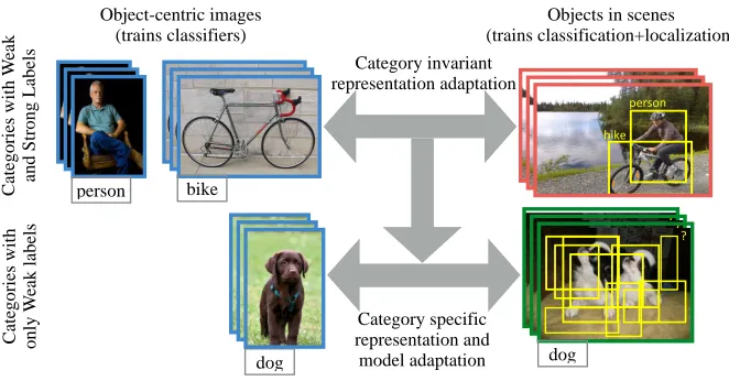
person' bike' ?" person' bike' person' bike' ?"?" Ca te gori es w it h W ea k and S trong L abe ls Ca te gori es w it h onl y W ea k l abe ls dog dog person bike Category invariant representation adaptation Category specific representation and model adaptation Object-centric images (trains classifiers)
Objects in scenes (trains classification+localization)
Figure 1: We learn detectors (models which classify and localize) for categories with only weak labels (bottom row). We use auxiliary categories with available paired strong and weak annotations (top row) to learn to adapt a visual representation from whole image classification to localized region detection. We then use the adapted representation to transform the classifiers trained for the categories with only weak labels and jointly solve an MIL problem to mine localized training data from the weakly labeled scene-centric training data (green – bottom right).
using the auxiliary strong labels to improve the feature representation for detection tasks, and uses the improved representation to learn a stronger detector from weak labels in a deep architecture.
We cast the task as a domain adaptation problem, considering the data used to train classifiers (images with category labels) as our source domain, and the data used to train detectors (images with bounding boxes and category labels) as our target domain. We then seek to find a general transformation from the source domain to the target domain, that can be applied to any image classifier to adapt it into a object detector (see Figure 1). R-CNN (Girshick et al., 2014) demonstrated that adaptation, in the form of fine-tuning, is very important for transferring deep features from classification to detection and partially inspired our approach. However, the R-CNN algorithm uses classification data only to pre-train a deep network and then requires a large number of bounding boxes to pre-train each detection category.
We additionally show that our large-scale detection models can be directly converted into models which produce pixel-level localization for each category. Following the recent result of Long et al. (2015), we run our models fully-convolutionally and directly use the learned detection weights to predict per-pixel labels.
We evaluate our detection model empirically on the largest set of available ground-truth visual data labeled with bounding box annotations, the ILSVRC13 detection dataset. Our method outperforms the previous best MIL-based approaches for weakly labeled detector learning (Wang et al., 2014) on ILSVRC13 (Russakovsky et al., 2014) by 200%. Our model is directly applicable to learning improved “detectors in the wild”, including categories in ImageNet but not in the ILSVRC13 detection dataset, or categories defined ad-hoc for a particular user or task with just a few training examples to fine-tune a new classification model. Such models can be promoted to detectors with no (or few) labeled bounding boxes. The article builds on two conference publications. The generic feature adaptation for transforming a classifier into a detector was first presented in Hoffman et al. (2014). Hoffman et al. (2015) presented a further category specific detector and representation refinement with mined localization labels. In this work, we present and compare the two works and ad-ditionally present a novel extension for further producing per-pixel predictions for adapting to the semantic segmentation task.
2. Related Work
Since its inception, the multiple instance learning (MIL) problem (Dietterich et al., 1997), or learning from a set of labels that specify at least one instance in a bag of instances, has been attempted in several frameworks, including Noisy-OR and boosting (Ali and Saenko, 2014; Zhang et al., 2005). However, most commonly, it has been framed as a max-margin classifi-cation problem (Andrews et al., 2002), with latent parameters optimized using alternating optimization (Felzenszwalb et al., 2010; Yu and Joachims, 2009).
While these approaches are promising, they often underperform on the full detection task in more challenging settings such as the PASCAL VOC dataset (Everingham et al., 2010), where objects only cover small portions of images, and many candidate bounding boxes contain no objects whatseover. The major challenges faced by solutions to the MIL problem are the limitations of fixed feature representations and poor initializations, particularly in non-object centric images. Our algorithm provides solutions to both of these issues. We also provide an evaluation on the large-scale ILSVRC13 detection dataset, which many previous methods have not been evaluated on.
Deep convolutional neural networks (CNNs) have emerged as state of the art on popular object classification benchmarks such as ILSVRC (Krizhevsky et al., 2012) and MNIST. In fact, “deep features” extracted from CNNs trained on the object classification task are also state of the art on other tasks such as subcategory classification, scene classification, domain adaptation (Donahue et al., 2014), and even image matching (Fischer et al., 2014). Unlike the previously dominant features (SIFT (Lowe, 2004), HOG (Dalal and Triggs, 2005)), deep CNN features can be learned for each specific task, but only if sufficient labeled training data is available. R-CNN (Girshick et al., 2014) showed that fine-tuning deep features, pre-trained for classification, on a large amount of bounding box labeled data significantly improves detection performance.
Domain adaptation methods aim to reduce dataset bias caused by a difference in the statistical distributions between training and test domains. In this paper, we treat the transformation of classifiers into detectors as a domain adaptation task. Many approaches have been proposed for classifier adaptation, such as feature space transformations (Saenko et al., 2010; Kulis et al., 2011; Gong et al., 2012; Fernando et al., 2013), model adaptation approaches (Yang et al., 2007a; Aytar and Zisserman, 2011), and joint feature and model adaptation (Hoffman et al., 2013a; Duan et al., 2012). However, even the joint learning models are not able to modify the feature extraction process and so are limited to shallow adaptation techniques. Additionally, these methods only adapt between visual domains, keeping the task fixed, while we adapt both from a large visual domain to a smaller visual domain and from a classification task to a detection task.
However, domain adaptation techniques have seen recent success through the merger with deep CNNs. Hoffman et al. (2013b) showed that, when training data in the target domain is severely limited or unavailable, domain adaptation techniques as applied to CNNs can be more effective than the standard practice of fine-tuning. More recent works have seen success in augmenting deep architectures with additional regularization layers that are robust to the negative effects of domain shift (Ghifary et al., 2014; Tzeng et al., 2014; Long and Wang, 2015; Ganin and Lempitsky, 2015). However, all of these methods focus on the standard visual domain adaptation problem, where one adapts between two versions of the same task with different statistics, and do not investigate the task adaptation setting.
an-notations for all object categories, both in the source and target domains, which is absent in our scenario.
Other methods have been proposed that use the underlying semantic hierarchy of Im-ageNet to transfer localization information to classes for strong labels are available (Guil-laumin and Ferrari, 2012; Vezhnevets and Ferrari, 2014). However, this necessarily limits their approaches to settings in which additional semantic information is available.
2.1 Background: MIL
We begin by briefly reviewing a standard solution to the multiple instance learning problem, Multiple Instance SVMs (MI-SVMs) (Andrews et al., 2002) or Latent SVMs (Felzenszwalb et al., 2010; Yu and Joachims, 2009). In this setting, each weakly labeled image is considered a collection of bounding boxes which form a positive ‘bag’. For a binary classification problem, the task is to maximize the bag margin which is defined by the instance with highest confidence. For each weakly labeled imageI ∈ W, we collect a set of bounding boxes and define the index set of those boxes as RI. We next define a bag as BI ={xi|i∈RI},
with label YI, and let theith instance in the bag be (xi, yi)∈ Rp× {−1,+1}.
For an image with a negative image-level label, YI =−1, we label all bounding boxes
in the image as negative. For an image with a positive image-level label, YI = 1, we create
a constraint that at least one positive instance occurs in the image bag.
In a typical detection scenario, RI corresponds to the set of possible bounding boxes
inside the image, and maximizing overRIis equivalent to discovering the bounding box that
contains the positive object. We define a representationφ(xi)∈ Rdfor each instance, which
is the feature descriptor for the corresponding bounding box, and formulate the MI-SVM objective as follows:
min
w∈Rd
1 2kwk
2 2+α
X
I
`YI,max i∈RI
wTφ(xi)
(1)
where αis a hyper-parameter and `(y,yˆ) is the hinge loss. Interestingly, for negative bags i.e. YI = −1, the knowledge that all instances are negative allows us to unfold the max
operation into a sum over each instance. Thus, Equation (1) reduces to a standard QP with respect tow. For the case of positive bags, this formulation reduces to a standard SVM if the maximum scoring instance is known.
Based on this idea, Equation (1) is optimized using a classic concave-convex proce-dure (Yuille and Rangarajan, 2003), which decreases the objective value monotonically with a guarantee to converge to a local minima or saddle point. Due to this reason, weakly trained MIL detectors are sensitive to the feature representation and initial detector weights (i.e. initialization in MIL) (Cinbis et al., 2014; Song et al., 2014a). With our algorithm we mitigate these sensitivities by learning a representation that works well for detection and by proposing an initialization technique for the weakly trained detectors which proves to avoid many of the pitfalls of prior MIL techniques (see Fig 7).
3. Large Scale Detection through Adaptation
is to cast the shift from tasks that require weak labels to tasks that require strong labels as a domain adaptation problem. We then consider transforming the models for the weakly labeled task into the models for the strongly labeled task. For concreteness, we will present our algorithm applied to the specific task shift of classification to detection, called Large Scale Detection through Adaptation (LSDA). In the following section, we will explain how to shift to a different strongly labeled task of semantic segmentation.
Let the set of images with only weak labels be denoted as W and the set of images with strong labels (bounding box annotations) from auxiliary tasks be denoted as S. We assume that the set of object categories that appear in the weakly labeled set,CW, do not
overlap with the set of object categories that appear in the strongly labeled set, CS. For
each image in the weakly labeled set, I ∈ W, we have an image-level label per category,
k: Yk
I ∈ {1,−1}. For each image in the strongly labeled set, I ∈ S, we have a label per
category,k, per region in the image,i∈RI: yik∈ {1,−1}. We seek to learn a representation,
φ(·) that can be used to train detectors for all object categories, C = {CW ∪ CS}. For a
category k ∈ C, we denote the category specific detection parameter as wk and compute
our final detection scores per region,x, asscorek(x) =wTkφ(x).
We propose a joint optimization algorithm which learns a feature representation, φ(·), and detection model parameters,wk, using the combination of strongly labeled scene-centric
data, S, with weakly labeled object and scene-centric data, W. For a fixed representation, one can directly train detectors for all categories represented in the strongly labeled set,
k∈CS. Additionally, for the same fixed representation, we reviewed in the previous section
techniques to train detectors for the categories in the weakly labeled data set, k ∈ CW.
Our insight is that the knowledge from the strong label set can be used to help guide the optimization for the weak labeled set, and we can explicitly adapt our representation for the categories of interest and for the generic detection task.
Below, we state our overall objective:
min
wk,φ
k∈C
X
k
Γ(wk) +α1 X
I∈W
X
p∈CW
F(YIp,wp) +α2 X
I∈S
X
i∈RI
X
q∈CS
`(yiq,wqTφ(xi)) (2)
where `(.) is the cross-entropy loss function, F is the region-based loss function over weak categories,α1, α2 are scalar hyper-parameters and Γ(.) is a regularization over the detector weights. We use convolutional neural networks (CNNs) to define our representationφ and thus the last layer weights serve as detection weightsw. We adopt the CNN architecture of Krizhevsky et al. (2012) (referred to as AlexNet).
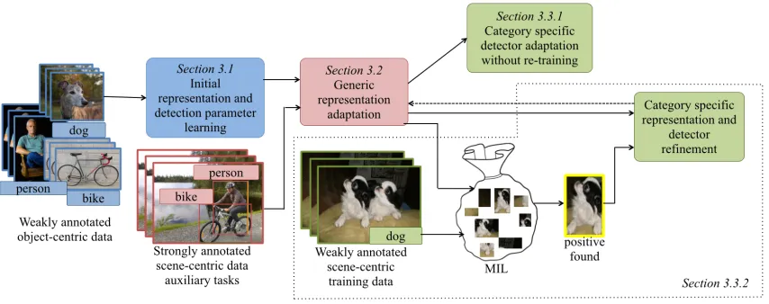
This formulation is difficult to optimize directly, so we propose to solve this objective by sequentially optimizing easier sub-problems which are less likely to diverge (see Figure 2).
Figure 2: Our method (LSDA) jointly optimizes a representation and category specific detection parameters for categories with only weakly labeled data. We first learn a feature representation conducive to adaptation by initializing all parameters with weakly labeled data. We then collectively refine the feature space with strongly labeled data from auxiliary tasks to adapt the category invariant representation from classification to detection (red boxes). Finally, we perform category specific adaptation (green boxes) either without re-training or by solving MIL in our detection feature space and using the discovered bounding boxes to further refine the representation and detection weights.
strongly labeled data from auxiliary tasks to jointly optimize all parameters corresponding to feature representation and detection weights. We now describe each of these steps in detail in the follow subsections.
3.1 Initializing representation and detection parameters
As mentioned earlier, we use the AlexNet architecture to describe representation φ and detection weights w. Since this network requires a large amount of data and time to train its approximately 60 million parameters, we start by pre-training on the ILSVRC2012 classification dataset, which we refer to as auxiliary weakly labeled data. It contains 1.2 million weakly labeled images of 1000 categories. Pre-training on this dataset has been shown to be a very effective technique (Donahue et al., 2014; Sermanet et al., 2013; Girshick et al., 2014), both in terms of performance and in terms of limiting the amount of in-domain labeled data needed to successfully tune the network. This data is usually object centric and is therefore effective for training a network that is able to discriminate between different categories. Next, we replace the last weight layer (1000 linear classifiers) with K = |C|
randomly initialized linear classifiers, one for each category in our task.
We next learn initial values for all of the detection parameters for our particular cat-egories of interest, wk, ∀k ∈ C. We obtain such initialization by solving the simplified
learning problem of image-level classification. The image, I ∈ S, is labeled as positive for a category kif any of the regions in the image are labeled as positive for k and is labeled as negative otherwise, we denote the image level label as in the weakly labeled case: Yk
I.
parameters that can be used per region proposal to produce detection scores:
min
wk,φ
k∈C
X
k
Γ(wk) +α
X
I∈{W∪S}
`(Yk
I,wTkφ(I))
(3)
We optimize Equation (3) through fine-tuning our CNN architecture with a newK-way last fully connected layer, whereK =|C|. This serves as our initialization for solving sequential sub-problems to optimize overall objective (2). We find that even using the net trained on weakly labeled data in this way produces a strong baseline. We will refer this baseline as ‘Classification Network’ in the experiments; see Table 2.
3.2 Learning category specific representation and detection parameters
We next transform our classification network into a detection network and learn a represen-tation which makes it possible to separate objects of interest from background and makes it easy to distinguish different object categories. We proceed by modifying the representation (layers 1-7),φ(·), through finetuning, using the available strongly labeled data for categories in setCS. Following the Regions-based CNN (R-CNN) (Girshick et al., 2014) algorithm, we
collect positive bounding boxes for each category in set CS as well as a set of background
boxes using a region proposal algorithm, such as selective search (Uijlings et al., 2013). We use each labeled region as a fine-tuning input to the CNN after padding and warping it to the CNN’s input size. Note that the R-CNN fine-tuning algorithm requires bounding box annotated data for all categories and so can not directly be applied to train all K
detectors. Fine-tuning transforms all network weights (except for the linear classifiers for categories in CW) and produces a softmax detector for categories in set CS, which includes
a weight vector for the new background class. We find empirically that fine-tuning induces a generic, category invariant transformation of the classification network into a detection network. That is, even though fine-tuning sees no strongly labeled data for categories in set
CW, the network transforms in a way that automatically makes the original set CW image
classifiers much more effective at detection (see Figure 9). Fine-tuning for detection also learns a background weight vector that encodes a generic “background” category,wb. This
background model is important for modeling the task shift from image classification, which does not include background distractors, to detection, which is dominated by background patches. This detector explicitly attempts to recognize all data labeled as negative in our bags. Since we initialize this detector with the strongly labeled data, we know precisely which regions correspond to background.
This can be summarized as the following intermediate sub-problem for objective (2):
min
wq,φ
q∈{CS,b}
X
q
"
Γ(wq) +α
X
I∈S
X
i∈RI
`(yiq,wTqφ(xi))
#
(4)
3.3 Adapting category specific representation and detection parameters
Finally, we seek to adapt the category dependent representation and model parameters for the categories in our weakly labeled set,CW. We will present two approaches to this problem
of learning detection weights for weak categories. Specifically, we aim to update the weakly labeled category specific parameters. Section 3.3.1 presents a heuristic adaptation approach that requires no further CNN training with gradient descent and updates only the weakly labeled classification parameters. Section 3.3.2 describes a separate adaptation approach that directly optimizes a subproblem of our overall objective (2). It uses multiple instance learning to discover localized labeled regions in the weakly labeled training data and uses the discovered labels to adapt both the representation and the classification parameters for categories in the weakly labeled set.
3.3.1 K-nearest neighbors based adaptation
In this section, we describe a technique for adapting the category specific parameters of the classifier model into the detector model parameters that are better suited for use with the detection feature representation based on a k-NN heuristic. We will determine a simi-larity metric between each category in the weakly labeled set, CW, to the strongly labeled
categories,CS.
For simplicity, we separate the category specific output layer (8th layer of the network
-f c8) of the classification model into two componentsf cS andf cW, corresponding to model
parameters for the categories in the strongly labeled set CS and the weakly labeled set
CW, respectively. During our generic category adaptation of Section 3.1, we trained a new
background prediction layer, f cb.
For categories in set CS, adaptation to detectors can be learned directly through
fine-tuning the category specific model parameters f cS. This is equivalent to fixing f cS and
learning a new layer, zero initialized, δS, with equivalent loss to f cS, and adding together
the outputs of δS and f cS.
Let us define the weights of the output layer of the original classification network asWc,
and the weights of the output layer of the adapted detection network asWd. We know that
for a category i∈ CS, the final detection weights should be computed as Wid=Wic+δSi.
However, since there is no strongly labeled data for categories in CW, we cannot directly
learn a corresponding δW layer during tuning. Instead, we can approximate the fine-tuning that would have occurred to f cW had strongly labeled data been available. We do
this by finding the nearest neighbors categories in set CS for each category in set CW and
applying the average change. We assume that there are categories in setCS that are similar
to those in setCW and therefore have similar weights and similar gradient descent updates.
Here we define nearest neighbors as those categories with the nearest (minimal Euclidean distance) `2-normalizedf c8 parameters in the classification network. This corresponds to the classification model being most similar and hence, we assume, the detection model should be most similar. We denote the kth nearest neighbor in setC
S of category j ∈ CW
asNS(j, k), then we compute the final output detection weights for categories in setCW as:
∀j∈ CW :Wjd = Wjc+
1
k
k
X
i=1
Thus, we adapt the category specific parameters even without bounding boxes for categories in set CW. In section 5 we experiment with various values of k, including taking the full
average: k=|CS|. We will now refer to this method as ‘LSDA rep+kNN’ in our experiments.
3.3.2 MIL training based adaptation
The previous section provides a technique for adapting the category specific model param-eters for the weakly labeled categories without any further CNN training. However, we may want to modify our representation and model parameters by explicitly retraining with the weakly labeled data. To do this, we need to discover localization information from the image-level labels. Therefore, we will begin by solving a multiple instance learning (MIL) problem to discover the portion of each image most likely corresponding to the weak image-level label.
With the representation, φ, that has now been directly tuned for detection, we fix the parameter weights, φ(·) and solve for the regions of interest in each weak labeled image. This corresponds to solving the following objective:
min
wp
p∈{CW,b}
X
p
"
Γ(wp) +α
X
I∈W
F(YIp,wp)
#
(6)
F = max
i∈RI
wTpφ(xi) (7)
Note, we can decouple this optimization problem and independently solve for each category in our weakly labeled data set, p ∈ CW. Let’s consider a single category p. Our goal is to
minimize the loss for category p over images I ∈ W. We will do this by considering two cases. First, ifpis not in the weak label set of an image (YIp =−1), then all regions in that image should be considered negative for categoryp. Second, ifYIp = 1, then we positively label a region xi if it has the highest confidence of containing object and negatively label
all other regions. We perform the discovery of this top region in two steps. At first, we narrow down the set of candidate bounding boxes using the score,wT
pφ(xi), from our fixed
representation and detectors from the previous optimization step. This set is then refined to estimate the most likely region to contain a positive instance in a Latent SVM formulation. The implementation details are discussed section 5.4.
Our final optimization step is to use the discovered bounding boxes from our weak dataset to refine our detectors and feature representation from the previous optimization step. This amounts to the subsequent step for minimization of the joint objective described in Equation (2). We collectively utilize the strong labels of images in S and estimated bounding boxes for the weakly labeled set,W, to optimize for detector weights and feature representation, as follows:
min
wk,φ
k∈{C,b}
X
k
"
Γ(wk) +α
X
I∈{W∪S}
X
i∈RI
`(yki,wTkφ(xi))
#
(8)
Thus, the overall non-convex objective (2) is first approximated through initialization in (3). This initialization is then used to solve the sequential optimization problems defined in (4) and (6). Further, we present two ways to solve (6): k-NN based heuristic approach in (5) and MIL-based re-training approach in (7).
The sub-problem defined in (4) decreases the loss for strongly labeled categories and (8) decreases the loss for both weak-strong categories. Thus, this ensures that the overall objective (2) decreases. The refined detector weights and representation can be used to discover the bounding box annotations for weakly labeled data again, and this process can be iterated over (see Figure 2). We discuss re-training strategies and evaluate the contribution of this final optimization step in Section 5.5.
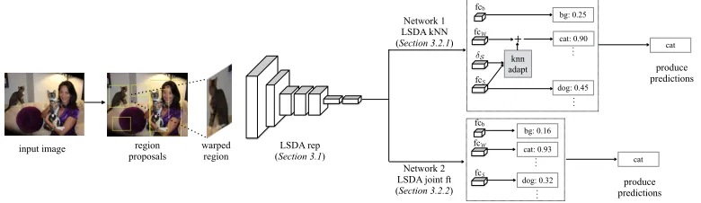
3.4 Detection with LSDA models
We now describe how our adapted network is used for detection at test time (depicted in Figure 3). For each test image we extract region proposals and generateK+ 1 scores per region (similar to the R-CNN (Girshick et al., 2014) pipeline), one score for each category and an additional score for the background category. The score is generated by passing the properly warped image patch through our adapted representation layers and then through one of our proposed category specific adapted layers (described in the previous sections). Finally, for a given region, the score for category i is computed by linearly combining the per category score with the background score: scorei−scorebg.
input image region
proposals warped region (Section 3.1)LSDA rep
fcb fcW knn adapt fcS S cat: 0.90 dog: 0.45 + bg: 0.25 fcb fcW fcS bg: 0.16 cat: 0.93 dog: 0.32 Network 1 LSDA kNN (Section 3.2.1) Network 2 LSDA joint ft (Section 3.2.2) … … … … produce predictions cat produce predictions cat
Figure 3: Detection with the LSDA network (test time). Given an image, extract region proposals, reshape the regions to fit into the network size and pass through our adapted network. Use the adapted representation and the category specific adaptation either through the no retraining nearest neighbor method or by retraining with our MIL based method. Finally produce detection scores per category for the region by considering background and category scores.
4. Recognition Beyond Detection
In the previous section we outline an algorithm for producing weakly supervised detection models which label and coarsely localize objects in scene-centric images. While a bounding box around an object offers significantly more information than an image-level label, it is not sufficiently localized for tasks such as robotic manipulation and full scene parsing. Instead, we would like to produce semantic segmentation models which are capable of labeling each pixel in an image with the object category or background label.
Prior work has shown that convolutional networks can also be applied to arbitrary-sized inputs to allow for per-pixel spatial output. For example, Matan et al. (1992) augmented the LeNet digit classification model (LeCun et al., 1989), enabling recognition of strings of digits, and Wolf and Platt (1994) use networks to output 2-dimensional maps in order to identify the locations of postal address blocks. This technique has been used to produce semantic segmentation outputs of C. elegans (Ning et al., 2005) and more recently for generic object categories (Long et al., 2015). These “fully convolutional” networks can also be finetuned end-to-end on segmentation ground truth to produce fully supervised segmentation models (Long et al., 2015).
As we would like to produce pixel level labels from our LSDA model, we will build off of our recent work for object category semantic segmentation (Long et al., 2015). However, Long et al. (2015) requires full semantic segmentation (pixel-level) annotations to train the corresponding fully connected network. This form of supervision is particularly expensive to collect and in general very few data sources exist with these annotations.
Instead, we argue that much of the knowledge gained through training with pixel-level annotations can be transferred from the much weaker bounding box annotations. There-fore, we demonstrate that a reasonable semantic segmentation is possible by directly using detection parameters in a fully convolutional framework. Further, we show that even our weakly supervised detection models presented in the previous section are able to localize objects more precisely than a bounding box, despite never receiving pixel-level annotations and for many categories never even receiving bounding box annotations.
To produce such a network we take our final adapted LSDA model, which for the purpose of our experiments was trained using an AlexNet basic architecture (Krizhevsky et al., 2012), and we convert the model into the corresponding fully convolutional 32 stride network (FCN-32s) presented by Long et al. (2015). This amounts to relatively few changes to the network architecture. First, each input image is paded with 100 pixels before features are extracted. Next each of the three fully connected layers are converted into convolutional layers, where layer 6 has 4096 convolutions with 6×6 sized kernels, layer 7 has 4096 convolutions with 1×1 sized kernels, and the final score layer hasK+ 1 convolutions with 1×1 sized kernels (where
5. Experiments
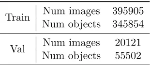
To demonstrate the effectiveness of our approach we present quantitative results on the ILSVRC2013 detection dataset. The dataset offers images exhaustively labeled with bound-ing box annotations for 200 relevant object categories. The trainbound-ing set has∼400K labeled images and on average 1.534 object classes per image. The validation set has 20K labeled images with ∼50K labeled objects. We simulate having access to weak labels for all 200 categories and having strong labels for only the first 100 categories (alphabetically sorted).
5.1 Experiment Setup & Implementation Details
We start by separating our data into classification and detection sets for training and a validation set for testing. Since the ILSVRC2013 training set has on average fewer objects per image than the validation set, we use this data as our classification data. To balance the categories we use ≈1000 images per class (200,000 total images). Note: for classification data we only have access to a single image-level annotation that gives a category label. In effect, since the training set may contain multiple objects, this single full-image label is a weak label, even compared to other classification training data sets. Next, we split the ILSVRC2013 validation set in half as (Girshick et al., 2014) did, producing two sets: val1 and val2. To construct our detection training set, we take the images with bounding box labels from val1 for only the first 100 categories (≈ 5000 images). Since the validation set is relatively small, we augment our detection set with 1000 bounding box labeled images per category from the ILSVRC2013 training set (following the protocol of (Girshick et al., 2014)). Finally we use the second half of the ILSVRC2013 validation set (val2) for our evaluation.
We implemented our CNN architectures and execute all fine-tuning using the open source software package Caffe (Jia et al., 2014) and have made our model definitions weights publicly available.
Train Num images 395905 Num objects 345854
Val Num images 20121 Num objects 55502
Table 1: Statistics of the ILSVRC13 detection dataset. Training set has fewer objects per image than validation set.
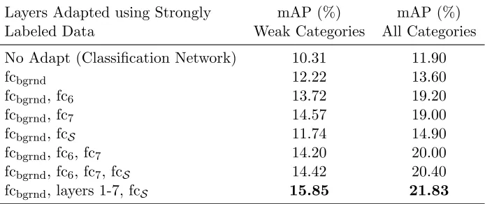
Layers Adapted using Strongly mAP (%) mAP (%) Labeled Data Weak Categories All Categories
No Adapt (Classification Network) 10.31 11.90
fcbgrnd 12.22 13.60
fcbgrnd, fc6 13.72 19.20
fcbgrnd, fc7 14.57 19.00
fcbgrnd, fcS 11.74 14.90
fcbgrnd, fc6, fc7 14.20 20.00
fcbgrnd, fc6, fc7, fcS 14.42 20.40
fcbgrnd, layers 1-7, fcS 15.85 21.83
Table 2: Ablation study for different techniques for category independent adaptation of our model (LSDA rep only). We consider training with the first 100 (alphabetically) categories of the ILSVRC2013 detection validation set (on val1) and report mean average precision (mAP) over the 100 weakly labeled categories (on val2). We find the best improvement is from fine-tuning all layers.
5.2 Quantitative Analysis of Adapted Representation
We evaluate the importance of each component of our algorithm through an ablation study. As a baseline, we consider training the network with only the weakly labeled data (no adaptation) and applying the network to the region proposals.
In Table 2, we present a detailed analysis of the different category independent adap-tation techniques we could use to train the network. We call this method LSDA rep only. We find that the best category invariant adaptation approach is to learn the background category layer and adapt all convolutional and fully connected layers, bringing mAP on the weakly labeled categories from 10.31% up to 15.85% i.e. this achieves a 54% relative mAP boost over the classification only network. We later observe that the most important step of our algorithm proved to be adapting the feature representation, while the least important was adapting the category specific parameter. This fits with our intuition that the main benefit of our approach is to transfer category invariant information from categories with known bounding box annotation to those without the bounding box annotations.
We find that one of the biggest reasons our algorithm improves is from reducing local-ization error. For example, in Figure 4, we show that while the classification only trained net tends to focus on the most discriminative part of an object (ex: face of an animal) after our adaptation, we learn to localize the whole object (ex: entire body of the animal).
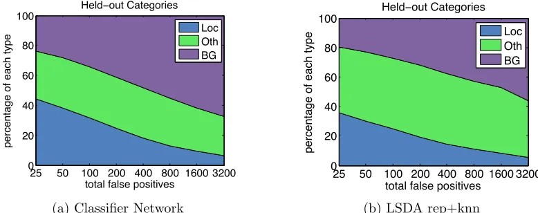
5.3 Error Analysis on Weakly Labeled Categories
Figure 4: We show example detections on weakly labeled categories, for which we have no detection training data, where LSDA (shown with green box) correctly localizes and labels the object of interest, while the classification network baseline (shown in red) incorrectly localizes the object. This demonstrates that our algorithm learns to adapt the classifier into a detector which is sensitive to localization and background rejection.
of errors found in each type as you look at the top scoring 25-3200 false positives.1 We con-sider the baseline of starting with the classification only network and show the false positive breakdown in Figure 5a. Note that the majority of false positive errors are confusion with background and localization errors. In contrast, after adapting the network using LSDA we find that the errors found in the top false positives are far less due to localization and background confusion (see Figure 5b). Arguably one of the biggest differences between clas-sification and detection is the ability to accurately localize objects and reject background. Therefore, we show that our method successfully adapts the classification parameters to be more suitable for detection.
total false positives
percentage of each type
Held−out Categories
25 50 100 200 400 800 1600 3200
0 20 40 60 80 100
Loc Oth BG
(a) Classifier Network
total false positives
percentage of each type
Held−out Categories
25 50 100 200 400 800 1600 3200
0 20 40 60 80 100
Loc Oth BG
(b) LSDA rep+knn
Figure 5: Comparison of error type breakdown on the categories which have no training bounding boxes available (weakly labeled data). After adapting all the layers in the network (LSDA), the percentage of false positive errors due to localization and background confusion is reduced (b) as compared to directly using the classification network for detection (a).
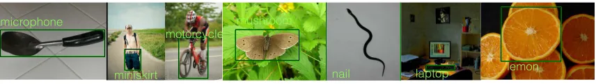
In Figure 6, we show examples of the top scoringOth error types for LSDA on the weakly labeled data. This means the detector localizes an incorrect object type. For example, the motorcycle detector localized and mislabeled bicycle and the lemon detector localized and mislabeled an orange. In general, we noticed that many of the top false positives from the
Oth error type were confusion with very similar categories. This is discussed in detail in next subsection.
microphone (sim): ov=0.00 1−r=−3.00
microphone
miniskirt (sim): ov=0.00 1−r=−1.00 miniskirt
motorcycle (sim): ov=0.00 1−r=−6.00 motorcycle
mushroom (sim): ov=0.00 1−r=−8.00
mushroom
nail (sim): ov=0.00 1−r=−4.00
nail
laptop (sim): ov=0.00 1−r=−3.00
laptop
lemon (sim): ov=0.00 1−r=−5.00 lemon
Figure 6: Examples of the top scoring false positives from our LSDA rep+knn network. Many of our top scoring false positives come from confusion with other categories.
5.4 Analysis of Discovered Boxes
We now analyze the quality of boxes discovered using adaptation of all layers including the background class. One of the key components of our system is using strong labels from auxiliary tasks to learn a representation where it’s possible to discover bounding boxes that correspond to the objects of interest in our weakly labeled data source. We begin our analysis by studying the bounding box discovery that our feature space enables, using selective search (Uijlings et al., 2013) to produce candidate regions. We optimize the bounding box discovery (Equations (6),(7)) using a one vs all Latent SVM formulation and optimize the formulation for AUC criterion (Bilen et al., 2014). This ensures that the top candidate regions chosen for joint fine-tuning have high precision. The feature descriptor used is the output of the fully connected layer,f c7, of the CNN which is produced after fine-tuning the feature representation with strongly labeled data from auxiliary tasks. Following our alternating minimization approach, these discovered top boxes are then used to re-estimate the weights and feature representations of our CNN architecture.
CorLoc over full dataset Localization mAP (%) ov=0.3 ov=0.5 ov=0.7 ov=0.9 ov=0.5
Classification Network 29.63 26.10 24.28 23.43 13.13 LSDA rep only 32.69 28.81 26.27 24.78 22.81
Table 3: CorLoc over dataset and localization mAP (i.e. given the labels) performance of discovered bounding boxes in our weakly labeled training set (val1) of ILSVRC13 detection dataset. Comparison with varying amount of overlap with ground truth box. About 25% of our discovered boxes have an overlap of at least 0.9. Our method is able to significantly improve the quality of discovered boxes after incorporating strong labels from auxiliary tasks.
metric. Table 3 reports the CorLoc for varying overlapping thresholds. CorLoc across full dataset is defined as the accuracy of discovered boxes i.e. the accuracy that the box is correctly localized per image at different thresholds. Our optimization approach produces one positive bounding box per image with a weak label, and a discovered box is considered a true positive if it overlaps sufficiently with the ground truth box that corresponds to that label. Since each bounding box, once discovered, is considered an equivalent positive (regardless of score) for the purpose of retraining the ‘LSDA rep only’ model, this simple CorLoc metric is a good indication of the usefulness of our discovered bounding boxes. We note here that after re-training with our mined boxes the CorLoc will further improved, as indicated in the detection mAP reported in the next section. It is interesting that a significant fraction of discovered boxes have high overlap with the ground truth regions. For reference, we also computed the standard mean average precision over the discovered boxes for localization task i.e. when label is known. It is important to note that the improvement in localization mAP is much more significant than the CorLoc. This is because mAP is obtained by averaging over recall values, and the ‘LSDA rep only’ model achieves better overall recall than the ‘Classification Network’ model.
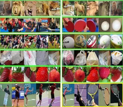
It is important to understand not only that our new feature space improves the quality of the resulting bounding boxes, but also what type of errors our method reduces. In Figure 7, we show the top 5 scoring discovered bounding boxes before and after modifying the feature space with strong labels from auxiliary tasks. We find that in many cases the improvement comes from better localization. For example without auxiliary strong labels we mostly discover the face of a lion rather than the body that we discover after our algorithm. Interestingly, there is also an issue with co-occurring classes. We are better able to localize “lion” body rather than the face. Most amazing results are for the “ping-pong” and “rugby” (second and third row) category where we are actually able to mine boxes for the racket and ball, while the classification net could only get the person boxes which is incorrect. Once we incorporate strong labels from auxiliary tasks we begin to be able to distinguish the person playing from the racket/ball itself. In the bottom row of Figure 7, we show the top 5 discovered bounding boxes for “tennis racket” where we are partially able to correct the images. Finally, there are some example discovered bounding boxes where we reduce quality after incorporating the strong labels from auxiliary tasks. For example, one of our strongly labeled categories is “computer keyboard”. Due to the strong training with keyboard images, some of our discovered boxes for “laptop” start to have higher scores on the keyboard rather than the whole laptop (see Figure 8). Also for the “water-craft” category, our adapted network ignores the mast but better localizes the boat itself. which slightly decreases the IOU of obtained box.
5.5 Detection Performance on ILSVRC13
Figure 7: Example discovered bounding boxes learned using our method. Left side shows the discovered boxes after fine-tuning with images in classification settings only, and right side shows the discovered boxes after fine-tuning with auxiliary strongly labeled dataset. We show top 5 discovered boxes across the dataset for corresponding category. Examples with a green outline are categories for which our algorithm was able to correctly discover bounding boxes of the object, while the feature space with only weak label training was not able to produce correct boxes. After incorporating the strong labels from auxiliary tasks, our method starts discovering “ping-pong” racket/ball and “rugby” ball, though still has some confusion with the person playing tennis. None of the discovered boxes from the original feature space correctly located racket/ball and instead included the person as well.
Inyellow we highlight the specific example of “tennis racket”, where some of the boxes get
(a) Non-adapted representation (b) Adapted representation (LSDA rep only)
Figure 8: Example discovered boxes of the category “laptop” where using auxiliary strongly labeled data causes bounding box discovery to diverge. Left: The discovered boxes obtained after fine-tuning with images in classification settings only. Right: The discovered boxes obtained after fine-tuning with the auxiliary strongly labeled dataset that contains the category “computer keyboard”. These boxes were low scoring examples, but we show them here to demonstrate a potential failure case – specifically, when one of the strongly labeled classes is a part of one of the weakly labeled classes. In the second example, adapted network better localizes the “water-craft” but misses the mast which decreases the IOU slightly.
LCL* Classification
Net
LSDA rep only
LSDA rep+kNN
LSDA rep+joint ft (all layers)
mAP (%)
0 2 4 6 8 10 12 14 16 18 20
6.00
10.31
15.85 16.15
18.08
*
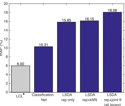
Figure 9: Comparison of mAP (%) for categories without any bounding box annotations (101-200 of val2) of ILSVRC13. The Joint representation and category-specific learning using MIL outperforms all other approaches. *As a reference we report the performance of LCL (Wang et al., 2014) which was computed across all 200 categories of the full validation set (val1+val2).
validation set. Our experiments indicate that the first 100 categories are easier on average then the second 100 categories, therefore the 6.0% mAP may actually be an upper bound of the performance of this approach. We also compare our algorithm against the scenario when the class-specific layer is adapted using nearest neighbors across all categories (LSDA rep+knn). The joint representation and multiple instance learning approach achieves the highest results (LSDA rep+joint ft).
Category Specific mAP (%) mAP (%) Adaptation Strategy Weak Categories All Categories
LSDA rep only 15.85 21.83
LSDA rep+kNN (k=5) 15.97 22.05
LSDA rep+kNN (k=10) 16.15 22.05
LSDA rep+kNN (k=100=|fcS|) 15.96 21.94
LSDA rep+joint ft (fcW) 17.01 22.43
LSDA rep+joint ft (all layers) 18.08 22.74
Baseline: Classification Network 10.31 11.90 Oracle: RCNN Full Detection Network 26.25 28.00
Table 4: Comparison of different ways to re-train after discovery of bounding boxes. We show mAP on val2 set from ILSVRC13. We find that the most effective way to re-train with discovered boxes is to modify the detectors and the feature representation.
mean average precision (mAP) percentage for no re-training (directly using the feature space learned after incorporating the strong labels), LSDA rep only, no retraining but last layer weights of weak categories adapted using nearest neighbors, LSDA rep+knn, re-training only the category-specific detection parameters, LSDA rep+joint ft (fcW), and retraining feature
representations jointly with category-specific weights, LSDA rep+joint ft (all layers). In our experiments the improved performance is due to the first iteration of the overall algorithm. We find that the best approach is to jointly learn to refine the feature representation and the category-specific detection weights. More specifically, we learn a new feature representation by fine-tuning all fully connected layers in the CNN architecture. The last row shows the performance achievable by our detection network if it had access to bounding box annotated data for all 200 categories, and serves as a performance upper bound.2 Our method achieves 18.08% mAP on weakly labeled categories as compared to 10.31% of baseline, but it is still significantly lower than fully-supervised oracle which gives 26.25%.
We finally analyze examples where our full algorithm which jointly learns representa-tion and class-specific layer using MIL (LSDA rep+joint ft) outperforms the previous ap-proach where only representation is adapted without joint learning over weak labels (LSDA rep+knn). Figure 10 shows a sample of the types of errors our algorithm improves on. These include localization errors, confusion with other categories, and interestingly, confu-sion with co-occurring categories. In particular, our algorithm provides improvement when searching for a small object (ball or helmet) in a sports scene. Training only with weak labels causes the previous state-of-the-art to confuse the player and the object, resulting in a detection that includes both. Our algorithm is able to localize only the small object and recognize that the player is a separate object of interest.
miniskirt rabbit
volleyball
watercraft soccerball
swine
monkey
lion mallot
rabbit
swine
volleyball
watercraft
monkey
volleyball
Figure 10: Examples where our algorithm after joint MIL adaptation (LSDA rep+joint ft) outperforms the representation only adaptation (LSDA rep only). We show the top scoring detection from LSDA rep only with aRedbox and label, and the top scoring detection from LSDA rep+joint ft, as a Green box and label. Our algorithm improves localization (ex: rabbit, lion etc), confusion with other categories (ex: miniskirt vs maillot), and confusion with co-occurring classes (ex: volleyball vs volleyball player)
5.6 Large Scale Detection
To showcase the capabilities of our technique we produced a 7604 category detector. The first categories correspond to the 200 categories from the ILSVRC2013 challenge dataset which have bounding box labeled data available. The other 7404 categories correspond to leaf nodes in the ImageNet database and are trained using the available full image weakly labeled classification data. We trained a full detection network using the 200 strongly labeled categories and trained the other 7404 last layer nodes using only the weak labels. Note, the ImageNet dataset does contain other non-exhausitvely labeled images for around 3000 object categories, 1825 of which overlap with the 7404 leaf node categories in our model. We do not use these labels during training of our large scale model. Quantitative evaluation for these categories is difficult to compute since they are not exhaustively labeled, however a followup work by Mrowca et al. (2015) evaluated F1 score of our model for the few object instances labeled per image to be 9.59%. Also note that while we have no bounding box annotations for the 7404 fine-grained categories, some may be related to the 200 basic level categories for which we use bounding box data to train – for example a particular breed of dog from 7404 weakly labeled data while ‘dog’ appears in the 200 strongly labeled categories.
We show qualitative results of our large scale detector by displaying the top detections per image in Figure 11. The results are filtered using non-max suppression across categories to only show the highest scoring categories.
American bison: 7.0
taillight: 0.9
wheel and axle: 1.0car: 6.0
whippet: 2.0
dog: 4.1
sofa: 8.0
Figure 11: Example top detections from our 7604 category detector. Detections from the 200 categories that have bounding box training data available are shown in blue. Detections from the remaining 7404 categories for which only weakly labeled data is available are shown in red.
computation. We have therefore also implemented and released a version of our algorithm running with fast region proposals (Kr¨ahenb¨uhl and Koltun, 2014) on a spatial pyramid pooling network (He et al., 2014), reducing our detection time down to half a second per image (from 4s per image) with nearly the same performance. We hope that this will allow the use of our 7.6K model on large data sources such as videos. We have released the 7.6K model and code to run detection (both the way presented in this paper and our faster version) atlsda.berkeleyvision.org.
5.7 Fully Convolutional LSDA for Semantic Segmentation
Bounding boxes localize objects to an inherently limited degree. While the system presented so far produces remarkably accurate bounding boxes from weak training labels, it does not address the ultimate goal of knowing exactly which pixels correspond to which objects.
Segmentation ground truth is unavailable for all but a few of the 7604 categories in our large scale detector, and segmentations are even more costly to annotate than bounding boxes. Nevertheless, as described in Section 5.7, we can convert our detection-adapted network into a fully-convolutional model following Long et al. (2015) and produce dense outputs for each of the 7604 categories plus 1 for background. We call this model LSDA7k FCN-32s since we use the 32 stride version of the fully convolutional networks proposed in Long et al. (2015). We next evaluate our semantic segmentation model using the PASCAL dataset Everingham et al. (2010) and the following metrics.
Metrics We compute both the commonly used mean intersection over union (mean IU) metric for semantic segmentation as well as three other metrics used by Long et al. (2015). The metrics are defined below, wherenij denotes the number of pixels from classipredicted
to belong to class j so that the number of pixels belonging to class iaremi =Pjnij, and
K denotes the number of classes.
• pixel accuracy: P
inii/Pimi
• mean accuracy: 1/KP
inii/ti
• mean IU: 1/KP
inii/(mi+
P
• frequency weighted IU: (P
lml)−1Piminii/(mi+Pjnji−nii)
We would like to understand how well our model can localize weakly trained objects so for each of the PASCAL 20 object categories we manually find the set of fine-grained categories from the 7404 weakly labeled leaf nodes in ImageNet that correspond to that category. Since layer 8 of our LSDA7k FCN-32s network produces 7605 outputs per region of the image, we insert an additional mapping layer which for each categorycis the maximum score across all weakly labeled categories which correspond to that PASCAL category. Next, this reduced score map where each image region now has 21 scores is run through the deconvolution layer to produce the corresponding PASCAL per pixel scores. Finally, for each pixel we choose a label based on which of the categories or background has the highest pixel score.
We report results on both the PASCAL 2011 and 2012 validation sets. Note, our method was not trained on any PASCAL images and in general was trained for classification of 7404 fine-grained categories and then adapted using our algorithm for detection. Additionally, our model is trained using the AlexNet architecture while most state-of-the-art semantic segmentation models are trained using the larger VGG network (Simonyan and Zisserman, 2014).
For the PASCAL 2011 validation set, shown in Table 5, we first compare against the classification model trained for the 7404 category full image labels. We run this model fully convolutionally using the FCN-32s approach (AlexNet) and report the segmentation performance in the first row as Classification 7K FCN-32s (AlexNet). This method gives a baseline for our LSDA approach which uses this model as the initialization prior to our adaptation approach. Next, we compare against the reported performance of the weakly trained models of Pathak et al. (2014) and for reference, the fully supervised AlexNet and VGG FCN-32s presented by Long et al. (2015). We report all four metrics for our work and report all available metrics for competing works. We see that our weakly trained model outperforms the baseline classification model run fully convolutionally and almost reaches the performance of the MIL-FCN method which uses the higher capacity VGG model and trains specifically for the segmentation task.
The per-category results of our method on the PASCAL 2012 validation set as compared to two state-of-the-art weakly trained semantic segmentation models is shown in Table 6. Not surprisingly, our LSDA7k FCN-32s underperforms these methods. No doubt adding the multiple instance loss of Pathak et al. (2014) or the object constraints of Pathak et al. (2015), while training directly on the PASCAL dataset would further improve our method. The purpose of these experiments is to give the reader an accurate picture of how well our large scale model performs at pixel level annotation without any tuning to the new situation.
We next show qualitative segmentation segmentation results across the fine-grained 7404 categories of our LSDA7k FCN-32s network in Figure 123 and compare against the baseline Classification 7K FCN-32s network. We find that often the segmentation masks from our LSDA network are more precise (see “American egret” example) and the top scoring predicted class is often more accurately labeled. For example, the bottom image is labeled as “air conditioner” by the classification network and correctly as “venetian blind” by our network. These category models were trained without ever seeing any associated
Scottish deerhound
Scotch terrier
American egret
American egret
iron horse
steam locomotive
catboat
lugger
Great Dane
levee
air conditioner
Venetian blind
Method pixel acc mean acc mean IU f.w. IU
Classification 7k FCN-32s (AlexNet) 13.3 43.2 11.6 6.7
MIL-FCN (VGG) (Pathak et al., 2014) - - 25.0
-LSDA7k FCN-32s (AlexNet) 70.6 35.5 21.3 59.2
FCN-32s (supervised AlexNet)(Long et al., 2015) 85.8 61.7 48.0 76.5
FCN-32s (supervised VGG)(Long et al., 2015) 89.1 73.3 59.4 81.4
Table 5: Semantic Segmentation Results for PASCAL 2011 validation set.
Method bgrnd aero bik
e
bird boat bottle bus car cat chair co
w
table dog horse mbik
e
p
e
rson
plan
t
sheep sofa train tv mean
EM Adapt (VGG) (Papandreou et al., 2015) 65.0 27.9 17.0 26.5 21.2 29.2 48.0 44.8 43.8 15.0 33.8 25.0 39.9 34.0 41.3 31.8 22.9 35.2 23.2 39.3 30.4 33.1
CCNN (VGG) (Pathak et al., 2015) 65.9 23.8 17.6 22.8 19.4 36.2 47.3 46.9 47.0 16.3 36.1 22.2 43.2 33.7 44.9 39.8 29.9 33.4 22.2 38.8 36.3 34.5
LSDA7k FCN-32s (AlexNet) 74.6 17.1 16.1 9.6 7.7 18.5 10.4 27.3 20.8 7.3 9.9 5.5 19.0 12.7 8.5 19.3 14.8 15.2 12.7 20.5 15.2 17.3
Table 6: Semantic Segmentation Results (mean IU%) for PASCAL 2012 validation set.
pixel-level annotations and only potentially see bounding box annotations for related classes (ex: a “dog” bounding box may be used in training but not a “dalmation”). We expect that further adaptation with a multiple instance loss or given a small amount of pixel-level semantic segmentation training data would further refine our models producing tigher object localization.
6. Conclusion
We have presented an algorithm that is capable of transforming a classifier into a detector. Our multi-stage algorithm uses corresponding weakly labeled (image-level annotated) and strongly labeled (bounding box annotated) data to learn the change from a classification CNN network to a detection CNN network, and applies that difference to future classi-fiers for which there is no available strongly labeled data. We then further demonstrate that our adapted detection models can be run fully convolutionally to produce a semantic segmentation model.
Our method jointly trains a feature representation and detectors for categories with only weakly labeled data. We use the insight that strongly labeled data from auxiliary tasks can be used to train a feature representation that is conducive to discovering bounding boxes in weakly labeled data. We demonstrate using a standard detection dataset (ILSVRC13 detection) that our method of incorporating the strongly labeled data from auxiliary tasks is very effective at improving the quality of the discovered bounding boxes. We then use all strong labels along with our discovered bounding boxes to further refine our feature representation and produce our final detectors. We show that our full detection algorithm significantly outperforms both the previous state-of-the-art methods which uses only weakly labeled data, as well as the algorithm which uses strongly labeled data from auxiliary tasks, but does not incorporate any MIL for the weak tasks.
adaptation algorithm. Given the significant improvement on the weakly labeled categories, our algorithm enables detection of tens of thousands of categories. We produce a 7.6K category detector and have released both code and models atlsda.berkeleyvision.org. Our approach significantly reduces the overhead of producing a high quality detector. We hope that in doing so we will be able to minimize the gap between having strong large-scale classifiers and strong large-large-scale detectors. Further we show that large-large-scale detectors can be used to produce large-scale semantic segmenters. We present semantic segmentation performance for the large scale model on PASCAL VOC with a manual mapping from the 7404 weakly labeled object categories to the 20 categories in the PASCAL dataset. For future work we would like to experiment with incorporating some pixel-level annotations for a few object categories. Our intuition is that by doing so we will be able to further improve our large-scale models with minimal extra supervision.
References
B. Alexe, T. Deselaers, and V. Ferrari. What is an object? InProc. CVPR, 2010.
K. Ali and K. Saenko. Confidence-rated multiple instance boosting for object detection. In IEEE Conference on Computer Vision and Pattern Recognition, 2014.
S. Andrews, I. Tsochantaridis, and T. Hofmann. Support vector machines for multiple-instance learning. InProc. NIPS, pages 561–568, 2002.
Y. Aytar and A. Zisserman. Tabula rasa: Model transfer for object category detection. In ICCV, 2011.
Y. Aytar and A. Zisserman. Enhancing exemplar svms using part level transfer regularization. In British Machine Vision Conference, 2012.
Y. Bengio, J. Louradour, R. Collobert, and J. Weston. Curriculum learning. In In Proc. ICML, 2009.
A. Berg, J. Deng, and L. Fei-Fei. ImageNet Large Scale Visual Recognition Challenge, 2012. URL http://www.image-net.org/challenges/LSVRC/2012/.
H. Bilen, V. P. Namboodiri, and L. J. Van Gool. Object and action classification with latent window parameters. IJCV, 106(3):237–251, 2014.
D. Borth, R. Ji, T. Chen, T. Breuel, and S. F. Chang. Large-scale visual sentiment ontology and detectors using adjective nown paiars. InACM Multimedia Conference, 2013.
R. G. Cinbis, J. Verbeek, C. Schmid, et al. Multi-fold mil training for weakly supervised object localization. InCVPR, 2014.
N. Dalal and B. Triggs. Histograms of oriented gradients for human detection. InIn Proc. CVPR, 2005.
T. Deselaers, B. Alexe, and V. Ferrari. Weakly supervised localization and learning with generic knowledge. IJCV, 2012.
J. Donahue, J. Hoffman, E. Rodner, K. Saenko, and T. Darrell. Semi-supervised domain adaptation with instance constraints. InComputer Vision and Pattern Recognition (CVPR), 2013.
J. Donahue, Y. Jia, O. Vinyals, J. Hoffman, N. Zhang, E. Tzeng, and T. Darrell. DeCAF: A Deep Convolutional Activation Feature for Generic Visual Recognition. InProc. ICML, 2014.
L. Duan, D. Xu, and I. W. Tsang. Learning with augmented features for heterogeneous domain adaptation. InProc. ICML, 2012.
M. Everingham, L. Van Gool, C. K. I. Williams, J. Winn, and A. Zisserman. The pascal visual object classes (voc) challenge. IJCV, 88(2):303–338, June 2010.
P. F. Felzenszwalb, R. B. Girshick, D. McAllester, and D. Ramanan. Object detection with discrim-inatively trained part-based models. IEEE Tran. PAMI, 32(9):1627–1645, 2010.
B. Fernando, A. Habrard, M. Sebban, and T. Tuytelaars. Unsupervised visual domain adaptation using subspace alignment. In Proc. ICCV, 2013.
P. Fischer, A. Dosovitskiy, and T. Brox. Descriptor matching with convolutional neural networks: a comparison to sift. ArXiv e-prints, abs/1405.5769, 2014.
C. Galleguillos, B. Babenko, A. Rabinovich, and S. Belongie. Weakly supervised object localization with stable segmentations. InECCV, 2008.
Y. Ganin and V. Lempitsky. Unsupervised Domain Adaptation by Backpropagation. In ICML, 2015.
M. Ghifary, W. B. Kleijn, and M. Zhang. Domain adaptive neural networks for object recognition. CoRR, abs/1409.6041, 2014. URLhttp://arxiv.org/abs/1409.6041.
R. Girshick, J. Donahue, T. Darrell, and J. Malik. Rich feature hierarchies for accurate object detection and semantic segmentation. In In Proc. CVPR, 2014.
D. Goehring, J. Hoffman, E. Rodner, K. Saenko, and T. Darrell. Interactive adaptation of real-time object detectors. InICRA, 2014.
B. Gong, Y. Shi, F. Sha, and K. Grauman. Geodesic flow kernel for unsupervised domain adaptation. InProc. CVPR, 2012.
M. Guillaumin and V. Ferrari. Large-scale knowledge transfer for object localization in imagenet. InCVPR, pages 3202–3209, June 2012. doi: 10.1109/CVPR.2012.6248055.
M. Guillaumin, D. Kttel, and V. Ferrari. Imagenet auto-annotation with segmentation propagation. IJCV, 110(3):328–348, 2014. ISSN 0920-5691. doi: 10.1007/s11263-014-0713-9. URL http: //dx.doi.org/10.1007/s11263-014-0713-9.
K. He, X. Zhang, S. Ren, and J. Sun. Spatial pyramid pooling in deep convolutional networks for visual recognition. InIn Proc. ECCV, 2014.
D. Hoeim, Y. Chodpathumwan, and Q. Dai. Diagnosing error in object detectors. InIn Proc. ECCV, 2012.
J. Hoffman, E. Tzeng, J. Donahue, Y. Jia, K. Saenko, and T. Darrell. One-shot adaptation of supervised deep convolutional models. CoRR, abs/1312.6204, 2013b. URL http://arxiv.org/ abs/1312.6204.
J. Hoffman, S. Guadarrama, E. Tzeng, R. Hu, J. Donahue, R. Girshick, T. Darrell, and K. Saenko. LSDA: Large scale detection through adaptation. In Neural Information Processing Systems (NIPS), 2014.
J. Hoffman, D. Pathak, T. Darrell, and K. Saenko. Detector discovery in the wild: Joint multiple instance and representation learning. InCVPR, 2015.
Y. Jia, E. Shelhamer, J. Donahue, S. Karayev, J. Long, R. Girshick, S. Guadarrama, and T. Darrell. Caffe: Convolutional architecture for fast feature embedding. arXiv preprint arXiv:1408.5093, 2014.
P. Kr¨ahenb¨uhl and V. Koltun. Geodesic object proposals. In In Proc. ECCV, 2014.
A. Krizhevsky, I. Sutskever, and G. E. Hinton. ImageNet classification with deep convolutional neural networks. InProc. NIPS, 2012.
B. Kulis, K. Saenko, and T. Darrell. What you saw is not what you get: Domain adaptation using asymmetric kernel transforms. In Proc. CVPR, 2011.
M. P. Kumar, B. Packer, and D. Koller. Self-paced learning for latent variable models. InIn Proc. NIPS, 2010.
Y. LeCun, B. Boser, J. Denker, D. Henderson, R. Howard, W. Hubbard, and L. Jackel. Backprop-agation applied to handwritten zip code recognition. Neural Computation, 1989.
J. Long, E. Shelhamer, and T. Darrell. Fully convolutional networks for semantic segmentation. CVPR, November 2015.
M. Long and J. Wang. Learning transferable features with deep adaptation networks. In ICML, 2015.
D. G. Lowe. Distinctive image features from scale-invariant key points. IJCV, 2004.
O. Matan, C. J. Burges, Y. L. Cun, and J. S. Denker. Multi-digit recognition using a space dis-placement neural network. In Neural Information Processing Systems, pages 488–495. Morgan Kaufmann, 1992.
D. Mrowca, M. Rohrbach, J. Hoffman, R. Hu, K. Saenko, and T. Darrell. Spatial semantic regular-isation for large scale object detection. InICCV, 2015.
F. Ning, D. Delhomme, Y. LeCun, F. Piano, L. Bottou, and P. E. Barbano. Toward automatic phenotyping of developing embryos from videos. In IEEE Transactions on Image Processing, pages 14(9):1360–1371, 2005.
M. Pandey and S. Lazebnik. Scene recognition and weakly supervised object localization with deformable part-based models. InProc. ICCV, 2011.
G. Papandreou, L.-C. Chen, K. Murphy, and A. L. Yuille. Weakly-and semi-supervised learning of a dcnn for semantic image segmentation. CoRR, abs/1502.02734, 2015.