Large Margin Semi-supervised Learning

Large Margin Semi-supervised Learning

Junhui Wang [email protected]

Xiaotong Shen [email protected]

School of Statistics University of Minnesota Minneapolis, MN 55455, USA

Editor: Tommi Jaakkola

Abstract

In classification, semi-supervised learning occurs when a large amount of unlabeled data is avail-able with only a small number of labeled data. In such a situation, how to enhance predictability of classification through unlabeled data is the focus. In this article, we introduce a novel large margin semi-supervised learning methodology, using grouping information from unlabeled data, together with the concept of margins, in a form of regularization controlling the interplay between labeled and unlabeled data. Based on this methodology, we develop two specific machines in-volving support vector machines andψ-learning, denoted as SSVM and SPSI, through difference convex programming. In addition, we estimate the generalization error using both labeled and unlabeled data, for tuning regularizers. Finally, our theoretical and numerical analyses indicate that the proposed methodology achieves the desired objective of delivering high performance in generalization, particularly against some strong performers.

Keywords: generalization, grouping, sequential quadratic programming, support vectors

1. Introduction

In many classification problems, a large amount of unlabeled data is available, while it is costly to obtain labeled data. In text categorization, particularly web-page classification, a machine is trained with a small number of manually labeled texts (web-pages), as well as a huge amount of unlabeled texts (web-pages), because manually labeling is impractical; compare with Joachims (1999). In spam detection, a small group of identified e-mails, spam or non-spam, is used, in conjunction with a large number of unidentified e-mails, to train a filter to flag incoming spam e-mails, compare with Amini and Gallinari (2003). In face recognition, a classifier is trained to recognize faces with scarce identified and enormous unidentified faces, compare with Balcan et al. (2005). In a situation as such, one research problem is how to enhance accuracy of prediction in classification by using both unlabeled and labeled data. The problem of this sort is referred to as semi-supervised learning, which differs from a conventional “missing data” problem in that the size of unlabeled data greatly exceeds that of labeled data, and missing occurs only in response. The central issue that this article addresses is how to use information from unlabeled data to enhance predictability of classification.

In semi-supervised learning, a sample_{Zi= (Xi,Yi)}i=nl1is observed with labeling Yi∈ {−1,1},

in addition to an independent unlabeled sample_{Xj}nj=nl+1with n=nl+nu, where Xk= (Xk1,···,

independently and identically distributed from distribution P(x)that may not be the marginal distri-bution of P(x,y).

A number of semi-supervised learning methods have been proposed through some assumptions relating P(x)to the conditional distribution P(Y=1_|X=x). These methods include, among others, co-training (Blum and Mitchell, 1998), the EM method (Nigam, McCallum, Thrun and Mitchell, 1998), the bootstrap method (Collins and Singer, 1999), information-based regularization (Szummer and Jaakkola, 2002), Bayesian network (Cozman, Cohen and Cirelo, 2003), Gaussian random fields (Zhu, Ghahramani and Lafferty, 2003), manifold regularization (Belkin, Niyogi and Sindhwani, 2004), and discriminative-generative models (Ando and Zhang, 2004). Transductive SVM (TSVM; Vapnik, 1998) uses the concept of margins.

Despite progress, many open problems remain. Essentially all existing methods make various assumptions about the relationship between P(Y =1_|X=x)and P(x)in a way for an improvement to occur when unlabeled data is used. Note that an improvement of classification may not be ex-pected when simply imputing labels of X through an estimated P(Y =1_|X=x)from labeled data, compare with Zhang and Oles (2000). In other words, the potential gain in classification stems from an assumption, which is usually not verifiable or satisfiable in practice. As a consequence, any departure from such an assumption is likely to degrade the “alleged” improvement, and may yield worse performance than classification with labeled data alone.

The primary objective of this article is to develop a large margin semi-supervised learning methodology to deliver high performance of classification by using unlabeled data. The method-ology is designed to adapt to a variety of situations by identifying as opposed to specifying a rela-tionship between labeled and unlabeled data from data. It yields an improvement when unlabeled data can reconstruct the optimal classification boundary, and yields a no worse performance than its supervised counterpart otherwise. This is in contrast to the existing methods.

Through three key ingredients, our objective is achieved, including (1) comparing all possible grouping boundaries from unlabeled data for classification, (2) using labeled data to determine label assignment for classification as well as a modification of the grouping boundary, and (3) interplay between (1) and (2) through tuning to connect grouping to classification for seeking the best classification boundary. These ingredients are integrated in a form of regularization involving three regularizers, each controlling classification with labeled data, grouping with unlabeled data, and interplay between them. Moreover, we introduce a tuning method using unlabeled data for tuning the regularizers.

Through the proposed methodology and difference convex programming, we develop two spe-cific machines based on support vector machines (SVM; Cortes and Vapnik, 1995) andψ-learning (Shen, Tseng, Zhang and Wong, 2003), denoted as SSVM and SPSI. Numerical analysis indicates that SSVM and SPSI achieve the desired objective, particularly against TSVM and a graphical method in simulated and benchmark examples. Moreover, a novel learning theory is developed to quantify SPSI’s generalization error as a function of complexity of the class of candidate decision functions, the sample sizes(nl,nu), and the regularizers. To our knowledge, this is the first attempt

to relate a classifier’s generalization error to(nl,nu) and regularizers in semisupervised learning.

This theory not only explains SPSI’s performance, but also supports our aforementioned discus-sion concerning the interplay between grouping and classification, as evident from Section 5 that SPSI can recover the optimal classification performance at a speed in nu because of grouping from

This article is organized in eight sections. Section 2 introduces the proposed semi-supervised learning methodology. Section 3 treats non-convex minimization through difference convex pro-gramming. Section 4 proposes a tuning methodology that uses both labeled and unlabeled data to enhance of accuracy of estimation of the generalization error. Section 5 presents some numerical ex-amples, followed by a novel statistical learning theory in Section 6. Section 7 contains a discussion, and the appendix is devoted to technical proofs.

2. Methodology

In this section, we present our proposed margin-based semi-supervised learning method as well its connection to other existing popular methodologies.

2.1 Proposed Methodology

We begin with our discussion in linear margin classification with labeled data (Xi,Yi)ni=l1 alone. Given a class of linear decision functions of the form f(x) =w˜T_fx+wf,0≡(1,xT)wf, a cost function

C∑nl

i=1L(yif(xi)) +J(f)is minimized with respect to f ∈

F

, a class of candidate decision functions, to obtain the minimizer ˆf yielding a classifier Sign(_fˆ_{), where J(f) =kw˜fk}2_{/2 is the reciprocal of} the L2 geometric margin, and L(·) is a margin loss defined by functional margins zi =yif(xi);

i=1,_···,nl.

Different learning methodologies are defined by different margin losses. Margin losses include, among others, the hinge loss L(z) = (1₋z)+ for SVM with its variants L(z) = (1₋z)q₊ for q>

1; compare with Lin (2002); the ρ-hinge loss L(z) = (ρ₋z)+ for nu-SVM (Sch ¨olkopf, Smola,

Williamson and Bartlett, 2000) withρ>0 to be optimized; theψ-loss L(z) =ψ(z), withψ(z) =

1−Sign(z)if z≥1 or z<0, and 2(1−z)otherwise, compare with Shen et al. (2003), the logistic loss L(z) =log(1+e−z), compare with Zhu and Hastie (2005); the sigmoid loss L(z) =1₋tanh(cz); compare with Mason, Baxter, Bartlett and Frean (2000). A margin loss L(z)is said to be a large margin if L(z)is nonincreasing in z, which penalizes small margin values.

In order to extract useful information about classification from unlabeled data, we construct a loss U(_·)for a grouping decision function g(x) = (1,xT)wg≡w˜Tgx+wg,0, with Sign(g(x))indicating grouping. Towards this end, we let U(z) =min_{y=±1}L(yz)by minimizing y in L(·)to remove its

dependency of y. As shown in Lemma 1, U(z) =L(_|z_|), which is symmetric in z and indicates that it can only determine the grouping boundary that occurs near in an area with low value of U(z)but provide no information regarding labeling.

While U can be used to extract the grouping boundary, it needs to yield the Bayes decision function f∗=arg minf∈FEL(Y f(X))in order for it to be useful for classification, where E is the

expectation with respect to(X,Y). More specifically, it needs f∗=arg ming∈FEU(g(X)).

How-ever, it does not hold generally since arg ming_∈F EU(g(X))can be any g∈

F

satisfying|g(x)| ≥1.

Generally speaking, U gives no information about labeling Y . To overcome this difficulty, we reg-ularize U and introduce our regreg-ularized loss for semi-supervised learning to induce a relationship between classification f and grouping g:

S(f,g;C) =C1L(y f(x)) +C2U(g(x)) +C3

2 kwf−wgk 2₊1

2kw˜gk

2_{, (1)}

data, U(g(x))controls the information extracted from unlabeled data, andkwf−wgk2penalizes the

disagreement between f and g, specifying a loose relationship between f and g. The interrelation between f and g is illustrated in Figure 3. Note that in (1) the geometric margin 2

kw˜fk2 does not enter

as it is regularized implicitly through 2

kwf−wgk2 and

2

kw˜gk2.

In nonlinear learning, a kernel K(_·,_·)that maps from S_×S to

R

1is usually introduced for flex-ible representations: f(x) = (1,K(x,x1),_···,K(x,xn))wf and g(x) = (1,K(x,x1),···,K(x,xn))wg

with wf = (w˜f,wf,0)and wg=w˜g+wg,0. Then nonlinear surfaces separate instances of two classes, implicitly defined by K(_·,_·), where the reproducing kernel Hilbert spaces (RKHS) plays an impor-tant role; compare with Wahba (1990) and Gu (2000). The forgoing treatment for the linear case is applicable when the Euclidean inner product_hxi,xjiis replaced by K(xi,xj). In this sense, the linear

case may be regarded as a special case of nonlinear learning.

Lemma 1 says that the regularized loss (1) allows U to yield precise information about the Bayes decision function f∗when after tuning. Specifically, U targets at the Bayes decision function in classification when C1 and C3 are large, and grouping can differ from classification at other C values.

Lemma 1 For any large margin loss L(z), U(z) =miny∈{−1,1}L(yz) =L(|z|), where y=Sign(z) =

arg miny_∈{−1,1}L(yz)for any given z. Additionally, (f_C∗,g_C∗) =arg inf

f,g∈FES(f,g;C)→(f

∗_,f∗_{) as C1,C3→∞.}

In the case that(f_C∗,g_C∗)is not unique, we choose it as any minimizer of ES(f,g;C). Through (1), we propose our cost function for semi-supervised learning:

s(f,g) =C1

nl

∑

i=1

L(yif(xi)) +C2 n

∑

j=nl+1

U(g(xj)) +

C3

2 kf−gk 2₊1

2kgk 2

−, (2)

where in the linear case, _kg_k− =_kw˜gkandkf−gk=kwf −wgk; in the nonlinear case kgk2₋=

˜

wT_gK ˜wg,kf−gk2= (w˜f−w˜g)TK(w˜f−w˜g)+(w˜f,0−w˜g,0)2is the RKHS norm, with an n×n matrix K whose i jth element is K(xi,xj). Minimization of (2) with respect to(f,g) yields an estimated

decision function ˆf thus classifier Sign(fˆ). The constrained version of (2), after introducing slack variables_{ξk≥0; k=1,···,n}, becomes

C1

nl

∑

i=1 ξi+C2

n

∑

j=nl+1

ξj+

C3

2 kf−gk 2₊1

2kgk 2

−, (3)

subject toξi−L(yif(xi))≥0; i=1,···,nl;ξj−U(g(xj))≥0; j=nl+1,···,n. Minimization of

(2) with respect to(f,g), equivalently, minimization of (3) with respect to(f,g,ξk; k=1,···,n)

subject to the constraints gives our estimated decision function(_fˆ_{,gˆ), where ˆf is for classification.} Two specific machines SSVM and SPSI will be further developed in what follows. In (2), SSVM uses L(z) = (1₋z)+and U(z) = (1− |z|)+, and SPSI uses L(z) =ψ(z)and U(z) =2(1− |z|)+.

2.2 Connection Between SSVM and TSVM

To better understand the proposed methodology, we now explore the connection between SSVM and TSVM. In specific, TSVM uses a cost function in the form of

C1

nl

∑

i=1

(1₋yif(xi))++C2

n

∑

j=nl+1

(1₋yjf(xj))++

1 2kfk

2

where minimization with respect to(yj: j=nl+1,···,n; f)yields the estimated decision function

ˆ

f . It can be thought of as the limiting case of SSVM as C3_→∞forcing f =g in (2).

SSVM in (3) stems from grouping and interplay between grouping and classification, whereas TSVM focuses on classification. Placing TSVM in the framework of SSVM, we see that SSVM relaxes TSVM in that it allows grouping (g) and classification (f) to differ, whereas f_≡g for TSVM. Such a relaxation yields that_|e(_fˆ_,f∗_)|=|GE(fˆ_)−GE(f∗_{)|is bounded by|e(f}ˆ_{,gˆ)|+|e(gˆ,g}∗

C)|+

|e(g∗_C,f∗)_|, with_|e(_fˆ_{,gˆ)|controlled by C3, the estimation error|e(gˆ,g}∗

C)|controlled by C2n−u1and

the approximation error_|e(g∗_C,f∗)_|controlled by C1and C3. As a result, all these error terms can be reduced simultaneously with a suitable choice of(C1,C2,C3), thus delivering better generalization. This aspect will be demonstrated by our theory in Section 6 and numerical analysis in Section 5. In contrast, TSVM is unable to do so, and needs to increase the size of one error in order to reduce the other error, and vice versa, compare with Wang, Shen and Pan (2007). This aspect will be also confirmed by our numerical results.

The forgoing discussion concerning SSVM is applicable to (2) with a different large margin loss L as well.

3. Non-convex Minimization Through Difference Convex Programming

Optimization in (2) involves non-convex minimization, because of non-convex U(z)and/or possi-bly L(z)in z. On the basis of recent advances in global optimization, particularly difference convex (DC) programming, we develop our minimization technique. Key to DC programming is decompo-sition of our cost function into a difference of two convex functions, based on which iterative upper approximations can be constructed to yield a sequence of solutions converging to a stationary point, possibly anε-global minimizer. This technique is called DC algorithms (DCA; An and Tao, 1997), permitting a treatment of large-scale non-convex minimization.

To use DCA for SVM andψ-learning in (2), we construct DC decompositions of the cost func-tions of SPSI and SSVM sψand sSV M in (2):

sψ=sψ₁₋sψ₂; sSV M=sSV M_{1 −}sSV M₂ ,

where L(z) =ψ(z)and U(z) =2(1_{− |}z_|)+for SPSI,

sψ₁ = C1∑nl

i=1ψ1(yif(xi)) +C2∑

n

j=nl+12U1(g(xj)) +

C3

2kf−gk2+ 1 2kgk2−,

sψ₂ = C1∑nl

i=1ψ2(yif(xi)) +C2∑

n

j=nl+12U2(g(xj));

and L(z) = (1₋z)+ and U(z) = (1− |z|)+ for SSVM,

sSV M₁ = C1∑nl

i=1(1−yif(xi))++C2∑

n

j=nl+1U1(g(xj)) +

C3

2kf−gk2+ 1 2kgk2−,

sSV M₂ = C2∑n_j=nl+1U2(g(xj)).

These DC decompositions are obtained through DC decompositions of(1_{− |}z_|)+=U1(z)−U2(z) andψ(z) =ψ1(z)−ψ2(z), where U1= (|z| −1)+, U2=|z| −1,ψ1=2(1−z)+, andψ2=2(−z)+.

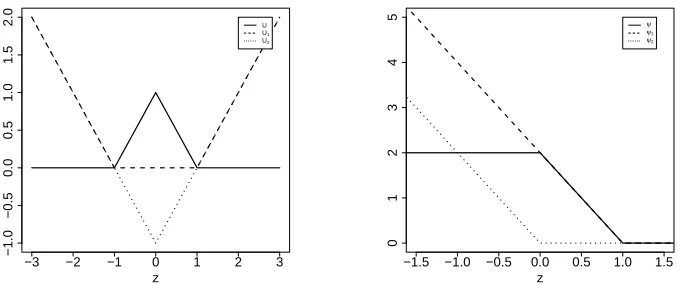
The decompositions are displayed in Figure 1.

With these decompositions, we treat the nonconvex minimization in (2) by solving a sequence of quadratic programming (QP) problems. Algorithm 1 solves (2) for SPSI and SSVM.

Algorithm 1: (Sequential QP)

−3 −2 −1 0 1 2 3

−1.0

−0.5

0.0

0.5

1.0

1.5

2.0

z

U

U1

U2

−1.5 −1.0 −0.5 0.0 0.5 1.0 1.5

0

1

2

3

4

5

z

ψ ψ1

ψ2

Figure 1: The left panel is a plot of U , U1and U2, for the DC decomposition of U=U1−U2. Solid, dotted and dashed lines represent U , U1and U2, respectively. The right panel is a plot of ψ,ψ1andψ2, for the DC decomposition ofψ=ψ1−ψ2. Solid, dotted and dashed lines representψ,ψ1andψ2, respectively.

and an precision tolerance levelε>0.

Step 2. (Iteration) At iteration k+1, compute (f(k+1),g(k+1)) by solving the corresponding dual problems given in (4).

Step 3. (Stopping rule) Terminate when_|s(f(k+1),g(k+1))₋s(f(k),g(k))_{| ≤}ε.

Then the estimate(fˆ,gˆ)is the best solution among(f(l),g(l))k+_l=11.

At iteration k+1, after omitting constants that are independent of (4), the primal problems are required to solve

min

wf,wg

sψ₁(f,g)_{− h}(f,g),∇sψ₂(f(k),g(k))_i,

min

wf,wg

sSV M₁ (f,g)_{− h}(f,g),∇sSV M₂ (f(k),g(k))_i. (4)

Here ∇sSV M₂ = (∇SV M

1 f ,∇SV M2 f ,∇SV M1g ,∇2gSV M) is the gradient vector of sSV M2 with respect to (f,g), with∇SV M_1g =C2∑n_j=nl+1∇U2(g(xj))xj,∇SV M_2g =C2∑nj=nl+1∇U2(g(xj)),∇

SV M

1 f =0p, and∇SV M2 f =0, where ∇U2(z) =1 if z>0, and ∇U2(z) =₋1 otherwise. Similarly, ∇sψ₂ = (∇ψ_{1 f},∇ψ_{2 f},∇ψ_1g,∇ψ_2g)

is the gradient vector of sψ₂ with respect to(wf,wg), with∇ψ1 f =C1∑i=nl1∇ψ2(yif(xi))yixi, ∇ψ2 f = C1∑n_i=l1∇ψ2(yif(xi))yi,∇ψ1g=2∇SV M1g , and∇

ψ

2g=2∇SV M2g , where∇ψ2(z) =0 if z>0 and∇ψ2(z) = −2 otherwise. By Karush-Kuhn-Tucker(KKT)’s condition, the primal problems in (4) are equivalent to their dual forms, which are generally easier to work with and given in the Appendix C.

By Theorem 3 of Liu, Shen and Wong (2005), lim

k→∞kf

(k+1)_−f(∞)_{k=0 for some f}(∞)_{, and}

con-vergence of Algorithm 1 is superlinear in that lim

k→∞kf

(k+1)_{− f}(∞)_k/kf(k)_{− f}(∞)_{k = 0 and}

lim

k→∞kg

(k+1)_−g(∞)_k/kg(k)_−g(∞)_{k=0, if there does not exist an instance ˜x such that f}(∞)_{(x˜) =}

g(∞)(x˜) = 0 with f(∞)(x) = (1,K(x,x1),···,K(x,xn))w(f∞) and g(∞)(x) = (1,K(x,x1),···, K(x,xn))wg(∞). Therefore, the number of iterations required for Algorithm 1 is o(log(1/ε)) to

4. Tuning Involving Unlabeled Data

This section proposes a novel tuning method based on the concept of generalized degrees of freedom (GDF) and the technique of data perturbation (Shen and Huang, 2006; Wang and Shen, 2006), through both labeled and unlabeled data. This permits tuning of three regularizers C= (C1,C2,C3)

in (2) to achieve the optimal performance.

The generalization error (GE) of a classification function f is defined as GE(f) =P(Y f(X)<

0) =EI(Y ₆=Sign(f(X))), where I(_·)is the indicator function. The GE(f)usually depends on the unknown truth, and needs to be estimated. Minimization of the estimated GE(f)with respect to the range of the regularizers gives the optimal regularization parameters.

For tuning, write ˆf as ˆfC, and write(Xl,Yl) = (Xi,Yi)_i=nl₁and Xu={Xj}n_j=nl+1. By Theorem 1

of Wang and Shen (2006), the optimal estimated GE(_fˆ_{C), after ignoring the terms independent of} ˆ

fC, has the form of

EGE(fˆC) + 1

2nl nl

∑

i=1

Cov(Yi,Sign(fˆC(Xi))|Xl) +

1 4D1(X

l_{,fˆC). (5)}

Here, EGE(_fˆ_{C) =} 1 2nl∑

nl

i=1(1−YiSign(fˆC(Xi)))is the training error, and D1(Xl,fˆC) =E E(4(X))−

1

nl∑

nl

i=14(Xi)|Xl

with ₄(X) = (E(Y_|X)₋Sign(_fˆ_C(X)))2_{, where E(·|X) and E(·|X}l_{) are}

condi-tional expectations with respect to Y and Yl respectively. As illustrated in Wang and Shen (2006), the estimated (5) based on GDF is optimal in the sense that it performs no worse than the method of cross-validation and other tuning methods; see Efron (2004).

In (5), Cov(Yi,Sign(fˆC(Xi))|Xl); i=1···,nl and D1(Xl,fˆC) need to be estimated. It appears

that Cov(Yi,Sign(fˆC(Xi))|Xl)is estimated only through labeled data, for which we apply the data

perturbation technique of Wang and Shen (2006). On the other hand, D1(Xl,fˆC)is estimated directly through(Xl,Yl)and Xujointly.

Our method proceeds as follows. First generate pseudo data Y_i∗by perturbing Yi:

Y_i∗=

Yi with probability 1−τ,

˜

Yi with probabilityτ, (6)

where 0<τ<1 is the size of perturbation, and (_Y˜_{i+1)/2 is sampled from a Bernoulli} distribu-tion with ˆp(xi), an rough probability estimate of p(xi) =P(Y =1_|X=xi), which may be obtained through the same classification method that defines ˆfCor through logistic regression when it doesn’t

yield an estimated p(x), such as SVM andψ-learning. The estimated covariance is proposed to be

d

Cov(Yi,Sign(fˆC(Xi))|Xl) =

1 k(Yi,pˆ(Xi))

Cov∗(Y_i∗,Sign(fˆ_C∗(Xi))|Xl); i=1,···,nl, (7)

where k(Yi,pˆ(Xi)) =τ+τ(1−τ)((Yi+1)/2−p(Xˆ i))

2 ˆ

p(Xi)(1−p(Xˆ i)) , and f

∗

C is an estimated decision function through

the same classification method trained through(Xi,Yi∗) nl

i=1.

To estimate D1, we express it as a difference between the true model error E(E(Y|X)− Sign(fˆC(X)))2 and its empirical version n−l 1∑

nl

be estimated through(Xl,Yl)and Xu. The estimated D1becomes

b

D1(Xl,_fˆ_{C) =E}∗ 1

nu n

∑

j=nl+1

((2 ˆp(Xj)−1)−Sign(fˆC∗(Xj)))2−

1 nl

nl

∑

i=1

((2 ˆp(Xi)−1)−Sign(fˆC∗(Xi)))2

X l ! , (8)

Generally, Cov in (7) andd D1b in (8) can be always computed using a Monte Carlo (MC) ap-proximation of Cov∗, E∗, when it is difficult to obtain their analytic forms. Specifically, when Yl is perturbed D times, a MC approximation ofCov andd Db1can be derived:

d

Cov(Yi,Sign(fˆC(Xi))|Xl)≈

1 D₋1

D

∑

d=1 1 k(Yi,pˆ(Xi))

Sign(_fˆ∗d

C (Xi))(Yi∗d−Y∗i), (9)

b

D1(Xl,fˆC)≈

1 D₋1

D

∑

d=1 1 nu n

∑

j=nl+1

((2 ˆp(Xj)−1)−Sign(fˆC∗d(Xj)))2−

1 nl

nl

∑

i=1

((2 ˆp(Xi)₋1)₋Sign(fˆ_C∗d(Xi)))2

!

,

where Y∗d

i ; d=1,···,D are perturbed samples according to (6), Y ∗

i = D1∑dYi∗d, and ˆfC∗d is trained

through(Xi,Yi∗d) nl

i=1. Our proposed estimateGE becomesc

c

GE(fˆC) =EGE(fˆC) +

1 2nl nl

∑

i=1 d

Cov(Yi,Sign(fˆC(Xi))|Xl) +

1 4Db1(X

l_,fˆ

C), (10)

By the law of large numbers, GE converges to (5) as Dc _→∞. In practice, we recommend D to be at least nl to ensure the precision of MC approximation andτto be 0.5. In contrast to the estimated

GE with labeled data alone, theGEc(fˆC)in (10) requires no perturbation of X when Xuis available. This permits more robust and computationally efficient estimation.

Minimization of (10) with respect to C yields the minimizer ˆC, which is optimal in terms of GE as suggested by Theorem 2, under similar technical assumptions as in Wang and Shen (2006).

(C.1): (Loss and risk) limnl→∞supC|GE(fˆC)/E(GE(fˆC))−1|=0 in probability.

(C.2): (Consistency of initial estimates) For almost all x, ˆpi(x)_→pi(x), as nl→∞; i=1,···,nl.

(C.3): (Positivity) Assume that inf

CE(GE(

ˆ

fC))>0.

Theorem 2 Under Conditions C.1-C.3, lim

nl,nu→∞

lim

τ→0+GE(

ˆ

fCˆ)/inf_C GE(fˆC)

=1.

5. Numerical Examples

This section examines effectiveness of SSVM and SPSI and compare them against SVM with la-beled data alone, TSVM and a graphical method of Zhu, Ghahramani and Lafferty (2003), in both simulated and benchmark examples. A test error, averaged over 100 independent replications, is used to measure their performances.

For simulation comparison, we define the amount of improvement of a method over SVM with labeled data alone as the percent of improvement in terms of the Bayesian regret,

(T(SV M)₋T(Bayes))₋(T(_·)₋T(Bayes))

T(SV M)₋T(Bayes) , (11)

where T(_·)and T(Bayes)are the test error of any method and the Bayes error. This metric seems to be sensible, which is against the baseline—the Bayes error T(Bayes), which is approximated by the test error over a test sample of large size, say 105.

For benchmark comparison, we define the amount of improvement over SVM as

T(SV M)₋T(_·)

T(SV M) , (12)

which underestimates the amount of improvement in absence of the Bayes rule.

Numerical analyses are performed in R2.1.1. For TSVM, SVMlight (Joachims, 1999) is used. For the graphical method, a MATLAB code provided in Zhu, Ghahramani and Lafferty (2003) is employed. In the linear case, K(s,t) =_hs,t_i; in the Gaussian kernel case, K(s,t) =exp₋ks−_σ2tk2

,

whereσ2is set to be p, a default value in the “svm” routine of R, to reduce computational cost for tuningσ2.

5.1 Simulations and Benchmarks

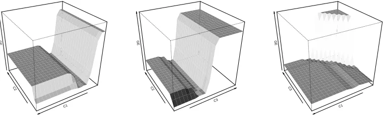
Two simulated and three benchmark examples are examined. In each example, we perform a grid search to minimize the test error of each classifier with respect to tuning parameters, in order to eliminate the dependency of the classifier on these parameters. Specifically, one regularizer for SVM and one tuning parameter σ in the Gaussian weight matrix for the graphical method, two regularization regularizers for TSVM, and three regularizers for SSVM and SPSI are optimized over [10−2,103]. For SSVM and SPSI, C is searched through a set of unbalanced grid points, based on our small study of the relative importance among(C1,C2,C3). As suggested by Figure 2, C3 appears to be most crucial to GEc(fˆC), whereas C2 is less important than (C1,C3), and C1 is only useful when its value is not too large. This leads to our unbalanced search over C, that is, C1∈ {10−2,10−1,1,10,102}, C2∈ {10−2,1,102}, and C3∈ {10m/4; m=−8,−7,···,12}. This strategy seems reasonable as suggested by our simulation. Clearly, a more refined search is expected to yield better performance for SSVM and SPSI.

Example 1: A random sample _{(Xi1,Xi2,Yi); i=1,···,1000} is generated as follows. First,

1000 independent instances(Yi,Xi1,Xi2)are sampled according to(Yi+1)/2∼Bernoulli(0.5), Xi1∼

Normal(Yi,1), and Xi2∼Normal(0,1). Second, 200 instances are randomly selected for training,

and the remaining 800 instances are retained for testing. Next, 190 unlabeled instances(Xi1,Xi2)

C2

C1 GE

C3

C2

GE

C3

C1 GE

Figure 2: Plot of GEc(_fˆ_{C) as a function of (C1,C2,C3) for one random selected sample of the} WBC example. The top left, the top right and the bottom left are plots of GEc(fˆC)

versus(C1,C2),(C2,C3) and(C3,C1), respectively. Here(C1,C2,C3)take values in set {10−2+m/4; m=0,1,_···,20_}.

Example 2: A random sample_{(Xi1,Xi2,Yi); i=1,···,1000}is generated. First, a random

sam-ple (Xi1,Xi2) of size 1000 is generated: Xi1 ∼ Normal(3 cos(kiπ/2 +π/8),1), Xi2 ∼

Normal(3 sin(kiπ/2+π/8),4), with ki sampled uniformly from {1,···,4}. Second, their labels

Yi; i=1,···,1000 are assigned: Yi=1 if ki∈ {1,4}, and−1 if ki∈ {2,3}. As in Example 1, we

obtain 200 (10 labeled and 190 unlabeled) instances for training as well as 800 instances for testing. The Bayes error is 0.089.

Benchmarks: Three benchmark examples are examined, including Wisconsin Breast Cancer (WBC), Mushroom and Spam email, each available in the UCI Machine Learning Repository (Blake and Merz, 1998). The WBC example concerns discrimination of a benign breast tissue from a malignant tissue through 9 clinic diagnostic characteristics; the Mushroom example separates an edible mushroom from a poisonous one through 22 biological records; the Spam email example discriminates texts to identify spam emails through 57 frequency attributes such as frequencies of particular words and characters. All these benchmarks are suited for linear and Gaussian kernel semi-supervised learning (Blake and Merz, 1998).

Instances in the WBC and Mushroom examples are randomly divided into halves with 10 labeled and 190 unlabeled instances for training, and the remaining instances for testing. Instances in the Spam email example are randomly divided into halves with 20 labeled and 580 unlabeled instances for training, and the remaining instances for testing.

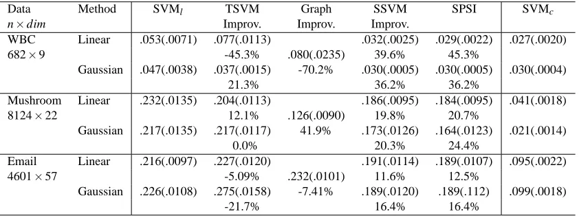
In each example, the smallest averaged test errors of SVM with labeled data alone, TSVM, the graphical method and our proposed methods are reported in Tables 1 and 2.

Data Method SVMl TSVM Graph SSVM SPSI SVMc

n×dim Improv. Improv. Improv. Improv.

Example 1 Linear .344(.0104) .249(.0134) .188(.0084) .184(.0084) .164(.0084) 1000×2 52.2% .232(.0108) 85.7% 87.9%

Gaussian .385(.0099) .267(.0132) 61.5% .201(.0072) .200(.0069) .196(.0015)

52.9% 82.5% 83.0%

Example 2 Linear .333(.0129) .222(.0128) .129(.0031) .128(.0031) .115(.0032) 1000_×2 45.5% .213(.0114) 83.6% 84.0%

Gaussian .347(.0119) .258(.0157) 49.2% .175(.0092) .175(.0098) .151(.0021)

34.5% 66.7% 66.7%

Table 1: Averaged test errors as well as the estimated standard errors (in parenthesis) of SVM with labeled data alone, TSVM, the graphical method, SSVM and SPSI, over 100 pairs of training and testing samples, in the simulated examples. Here Graph, SVMl and SVMc

denote performances of the graphical method, SVM with labeled data alone, and SVM with complete data without missing. The amount of improvement is defined in (11), where the Bayes error serves as a baseline for comparison.

Data Method SVMl TSVM Graph SSVM SPSI SVMc

n×dim Improv. Improv. Improv.

WBC Linear .053(.0071) .077(.0113) .032(.0025) .029(.0022) .027(.0020) 682×9 -45.3% .080(.0235) 39.6% 45.3%

Gaussian .047(.0038) .037(.0015) -70.2% .030(.0005) .030(.0005) .030(.0004)

21.3% 36.2% 36.2%

Mushroom Linear .232(.0135) .204(.0113) .186(.0095) .184(.0095) .041(.0018) 8124×22 12.1% .126(.0090) 19.8% 20.7%

Gaussian .217(.0135) .217(.0117) 41.9% .173(.0126) .164(.0123) .021(.0014)

0.0% 20.3% 24.4%

Email Linear .216(.0097) .227(.0120) .191(.0114) .189(.0107) .095(.0022) 4601×57 -5.09% .232(.0101) 11.6% 12.5%

Gaussian .226(.0108) .275(.0158) -7.41% .189(.0120) .189(.112) .099(.0018) -21.7% 16.4% 16.4%

Table 2: Averaged test errors as well as the estimated standard errors (in parenthesis) of SVM with labeled data alone, TSVM, the graphical method, SSVM and SPSI, over 100 pairs of training and testing samples, in the benchmark examples. The amount of improvement is defined in (12), where the performance of SVM with labeled data alone serves as a baseline for comparison in absence of the Bayes error.

• In the simulated examples, the improvements of SPSI and SSVM are from 66.9% to 87.9% over SVM, while the improvements of TSVM and the graphical method are from 34.5% to 52.9% and 49.2% to 61.5%, over SVM.

• In the benchmark examples, the improvements of SPSI, SSVM, TSVM, and the graphical method, over SVM, range from 19.8% to 45.3%, from -45.3% to 21.3%, and from -70.2% to 41.9%.

• SPSI and SSVM nearly reconstruct all relevant information about labeling in the two simu-lated examples and the WBC example, when they are compared with SVM with full label data. This suggests that room for further improvement in these cases is small.

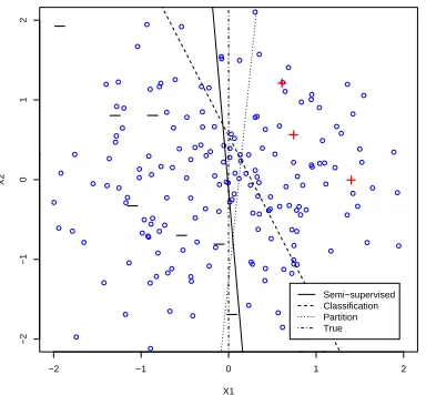
To understand how SPSI and SSVM perform, we examine one randomly chosen realization in Example 1 for SPSI. As displayed in Figure 3, SVM fails to provide an accurate estimate of the true decision boundaries, because of the small size of labeled data. In contrast, the grouping boundaries estimated by unlabeled covariates, almost recover the true decision boundaries for classification. This, together with the information obtained from the labeled data regarding the sign of labeling, results in much better estimated classification boundaries.

−2 −1 0 1 2

−2

−1

0

1

2

X1

X2

_

+

+

_

_ _

_ +

_ _

Semi−supervised Classification Partition True

Figure 3: Illustration of SPSI in one randomly selected replication of Example 1. The solid, dashed, dotted and dotted-dashed (vertical) lines represent ourψ-learning-based decision tion, the SVM decision function with labeled data alone, the partition decision func-tion defined by unlabeled data, and the true decision boundary for classificafunc-tion. Here C1=0.1, C2=0.01 and C3=0.5.

5.2 Performance After Tuning

This section compares the performances of the six methods in Section 5.1 when tuning is done using our proposed method in Section 4 and the training sample only. Particularly, SVM is tuned using the method of Wang and Shen (2006) with labeled data alone, and SPSI, SSVM , TSVM and the graphical method are tuned by minimizing the GEc(fˆC)in (10) involving both labeled and

unlabeled data over a set of grid points in the same fashion as in Section 5.1. Performances of all the methods are evaluated by a test error on an independent test sample. The averaged test errors of these methods are summarized in Table 3.

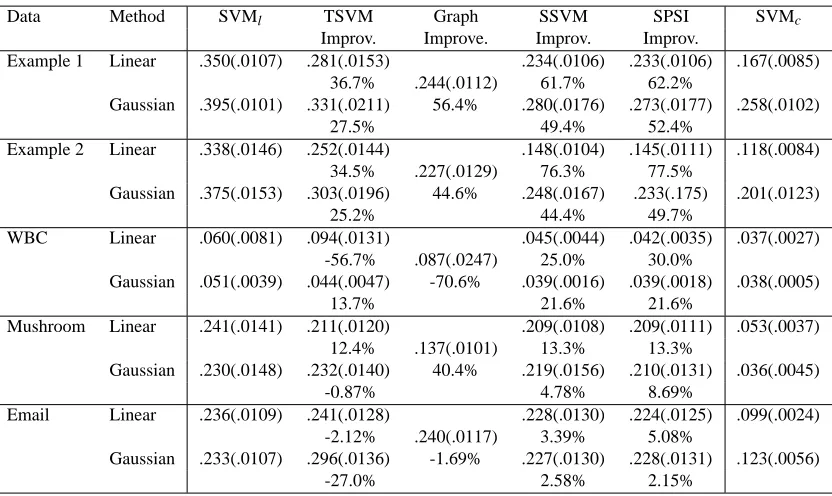
Data Method SVMl TSVM Graph SSVM SPSI SVMc

Improv. Improve. Improv. Improv.

Example 1 Linear .350(.0107) .281(.0153) .234(.0106) .233(.0106) .167(.0085) 36.7% .244(.0112) 61.7% 62.2%

Gaussian .395(.0101) .331(.0211) 56.4% .280(.0176) .273(.0177) .258(.0102)

27.5% 49.4% 52.4%

Example 2 Linear .338(.0146) .252(.0144) .148(.0104) .145(.0111) .118(.0084) 34.5% .227(.0129) 76.3% 77.5%

Gaussian .375(.0153) .303(.0196) 44.6% .248(.0167) .233(.175) .201(.0123)

25.2% 44.4% 49.7%

WBC Linear .060(.0081) .094(.0131) .045(.0044) .042(.0035) .037(.0027) -56.7% .087(.0247) 25.0% 30.0%

Gaussian .051(.0039) .044(.0047) -70.6% .039(.0016) .039(.0018) .038(.0005)

13.7% 21.6% 21.6%

Mushroom Linear .241(.0141) .211(.0120) .209(.0108) .209(.0111) .053(.0037) 12.4% .137(.0101) 13.3% 13.3%

Gaussian .230(.0148) .232(.0140) 40.4% .219(.0156) .210(.0131) .036(.0045) -0.87% 4.78% 8.69%

Email Linear .236(.0109) .241(.0128) .228(.0130) .224(.0125) .099(.0024) -2.12% .240(.0117) 3.39% 5.08%

Gaussian .233(.0107) .296(.0136) -1.69% .227(.0130) .228(.0131) .123(.0056) -27.0% 2.58% 2.15%

Table 3: Averaged test errors as well as the estimated standard errors (in parenthesis) of SVM with labeled data alone, TSVM, the graphical method, SSVM and SPSI after tuning, over 100 pairs of training and testing samples, for the simulated and benchmark examples.

In conclusion, our proposed methodology achieves the desired objective of delivering high per-formance and is highly competitive against the top performers in the literature, where the loss U(_·)

plays a critical role in estimating decision boundaries for classification. It is also interesting to note that TSVM obtained from SVMlight performs even worse than SVM with labeled data alone in the WBC example for linear learning, and the Spam email example for both linear and Gaussian ker-nel learning. One possible explanation is that SVMlight may not have some difficulty in reaching good minimizers for TSVM. Moreover, the graphical method compares favorably against SVM and TSVM, but its performance does not seem to be robust in different examples. This may be due to the required Gaussian assumption.

6. Statistical Learning Theory

This section derives a finite-sample probability upper bound measuring the performance of SPSI in terms of complexity of the class of candidate decision functions

F

, sample sizes (nl,nu) and

tuning parameter C. Specifically, the generalization performance of the SPSI decision function ˆfC

6.1 Assumptions and Theorems

Our statistical learning theory involves risk minimization and the empirical process theory. The reader may consult Shen and Wang (2006) for a discussion about a learning theory of this kind.

First we introduce some notations. Let(f_C∗,g_C∗) =arg inff,g∈F ES(f,g;C)is a minimizer for

surrogate risk ES(f,g;C), as defined in Lemma 1. Let ef =e(f,f∗)be the Bayesian regret for f

and eg=e(g,g_C∗)be the corresponding version for g relative to g_C∗. Denote by Vf(X) =L(Y f(X))−

L(Y f∗(X))and Vg(X) =U˜(g(X))−U˜(g∗C(X))be the differences between f and f∗, and g and gC∗

with respect to surrogate loss L and regularized surrogate loss ˜U(g) =U(g) + C3

2nuC2kg−f

∗ Ck2.

To quantify complexity of

F

, we define the L2-metric entropy with bracketing. Given anyε>0, denote_{(f_ml,f_mu)_}M

m=1as anε-bracketing function set of

F

if for any f ∈

F

, there exists an m such that f_ml _≤ f _≤ f_mu and_kf_ml ₋f_mu_k2≤ε; m=1,···,M, wherek · k2 is the usual L2 norm. Then the L2-metric entropy with bracketing H(ε,

F

)is defined as the logarithm of the cardinality of smallest ε-bracketing function set of

F

.

Three technical assumptions are formulated based upon local smoothness of L, complexity of

F

as measured by the metric entropy, and a norm relationship.

Assumption A. (Local smoothness: Mean and variance relationship) For some some constants 0<αh<∞, 0≤βh<2, aj>0; j=1,2,

sup

{h∈F: E(Vh(X))≤δ}

|eh| ≤a1δαh, (13)

sup

{h∈F: E(Vh(X))≤δ}

Var(Vh(X))_≤a2δβh_{, (14)}

for any smallδ>0 and h= f,g.

Assumption A describes the local behavior of mean (eh)-and-variance (Var(Vh(X))) relationship.

In (13), Taylor’s expansion usually leads toαh=1 when f and g can be parameterized. In (14), the

worst case isβh=0 because max(|L(y f)|,|U(g)|)≤2. In practice, values forαhandβhdepend on

the distribution of(X,Y).

Let J0=max(J(gC∗),1)with J(g) = 12kgk2− the regularizer. Let

F

l(k) ={L(y f)−L(y f∗): f ∈

F

,J(f)_≤k_}and

F

u(k) =_{U(g)₋U(g∗_C): g_∈

F

,J(g)_≤kJ0_}be the regularized decision function spaces for f ’s and g’s.

Assumption B. (Complexity) For some constants ai>0; i=3,···,5 andεnvwith v=l or u,

sup

k≥2

φv(εnv,k)≤a5n

1/2

v , (15)

where φu(ε,k) =

Ra

1/2 3 T

βg/2

u

a4Tu H

1/2_(w,

_F

u(k))dw/Tu with Tu = Tu(ε,C,k) = min(1,ε2/βg/2+ (nuC2)−1(k/2−1)J0), and φl(ε,k) = R

a1₃/2T_lβf/2 a4Tl H

1/2_(w,

_F

_l(k))dw/T

l with Tl = Tl(ε,C,k) =

min(1,ε2/βf_{/2+ (n}

lC1)−1(k/2−1)max(J(f∗),1)).

Although Assumption B is always satisfied by some εnv, the smallest possible εnv from (15)

yields the best possible error rate, for given

F

v and sample size nv. This is to say that the rate is

indeed governed by the complexity of

F

v(k). An equation of this type, originated from the empirical

Assumption C. (Norm relationship) For some constant a6>0,kfk1≤a6kfkfor any f ∈

F

, where_{k · k}1is the usual L1-norm.

Assumption C specifies a norm relationship between norm_{k · k}defined by a RKHS and_{k · k1}. This is usually met when

F

is a RKHS, defined, for instance, by Gaussian and Sigmoid kernels, compare with Adams (1975).

Theorem 3 (Finite-sample probability bound for SPSI) In addition to Assumptions A-C, assume that nl ≤nu. For the SPSI classifier Sign(fˆC), there exist constants aj>0; j=1,6,7,10,11, and

Jl>0, Ju>0 and B≥1 defined as in Lemma 5, such that

P inf

C |e(

ˆ

fC,f∗)| ≥a1sn

≤ 3.5 exp(₋a7nu((nuC2∗)−1J0)max(1,2−βg))+

6.5 exp(₋a10nl((nlC1∗)−1min(Jl,J(f∗)))max(1,2−βf))+

6.5 exp(₋a11nu((nuC2∗)−1Ju)max(1,2−βg)), where sn = min δ

2αf

nl ,max(δ

2αg

nu ,infC∈C|e(gC∗,f∗)|)

, δnv = min(εnv,1) with v = l,u, C∗ =

(C₁∗,C∗₂,C₃∗) = arg infC∈C|e(g∗C,f∗)|), and

C

= {C : nlC1 ≥ 2δ−nl2max(Jl,J(f

∗_),1),n uC2 ≥ 2δ−2

nu max(J0,2C3(2B+J(fC∗) +J(gC∗))),C3≥a

2 6Bδ−nu4}.

Corollary 4 Under the assumptions of Theorem 3, as nu≥nl→∞,

inf

C |e(

ˆ

fC,f∗)|=Op(sn), sn=min δ

2αf

nl ,max(δ

2αg

nu ,inf

C∈C|e(g ∗ C,f∗)|)

.

Theorem 3 provides a probability bound for the upper tail of_|e(_fˆ_C,f∗_{)|for any finite(n} l,nu).

Furthermore, Corollary 4 says that the Bayesian regret infC∈C|e(gC∗,f∗)| for the SPSI classifier

Sign(fˆC)after tuning is of order of no larger than sn, when nu≥nl →∞. Asymptotically, SPSI

per-forms no worse than its supervised counterpart in that infC|e(fˆC,f∗)|=Op(δ

2αf

nl ). Moreover, SPSI

can outperform its supervised counterpart in the sense that infC|e(fˆC,f∗)|=Op(min(δ

2αg

nu ,δ

2αf

nl )) =

Op(δ

2αg

nu ), when{gC∗ : C∈

C

}provides a good approximation to the Bayes rule f∗.

Remark: Theorem 3 and Corollary 4 continue to hold when the “global” entropy in (15) is replaced by a “local” entropy, compare with Van De Geer (1993). Let

F

_l,ξ(k) =_{L(y f)₋L(y f∗): f _∈

F

,J(f)_≤k,_|e(f,f∗)_{| ≤}ξ_} and

F

u,ξ(k) ={U(g)−U(gC∗): g∈

F

,J(g)≤k,|e(g,gC∗)| ≤ξ}

be the “local” entropy of

F

l(k)and

F

u(k). The proof requires only a slight modification. The local

entropy avoids a loss of log nufactor in the linear case, although it may not be useful in the nonlinear

case.

6.2 Theoretical Examples

We now apply the learning theory to one linear and one kernel learning examples to obtain the generalization error rates for SPSI, as measured by the Bayesian regret. We will demonstrate that the error in the linear case can be arbitrarily fast while that in the nonlinear case is fast. In either case, SPSI’s performance is better than that of its supervised counterpart.

Linear learning: Consider linear classification where X= (X(1),X(2))is sampled independently

probabilityτfor 0<τ< 1

2. Here the true decision function ft(x) =x(1)yielding the vertical line as

the classification boundary.

In this case, the degree of smoothness of this problem is characterized by exponentθ>0 in the density q(z), which describes the level of difficulty of linear classification but may not be so in the nonlinear case.

For classification, we minimize (2) over

F

, consisting of linear decision functions of form f(x) = (1,x)T_{w for w∈}

R

3 _{and x= (x}

(1),x(2))∈

R

2. To apply Corollary 4, we verify

Assump-tions A-C with detailed verification given in Appendix B. In fact, Assumption A follows from the smoothness of E(Vh(X))and Var(Vh(X))with respect to h, where a local Taylor expansion yields

the degree of smoothness exponentsαandβ. Assumption B is automatically met, and the entropy Equation (15) is solved for the smallest possible εnv satisfying it. Assumption C is always true

for RKHS. It then follows from Corollary 4 that infC|e(fˆC,f∗)|=Op(nu−(θ+1)/2(log nu)(θ+1)/2)as

nu≥nl→∞. This says that the optimal ideal performance of the Bayes rule is recovered by SPSI

at speed of n−u(θ+1)/2(log nu)(θ+1)/2as nu≥nl→∞. This rate is arbitrarily fast asθ→∞.

Kernel learning: Consider, in the preceding case, kernel learning with a different candidate decision function class defined by the Gaussian kernel. To specify

F

, we may embed a finite-dimensional Gaussian kernel representation into an infinite-finite-dimensional space

F

=_{x∈

R

2_{: f(x) =} wT_fφ(x) =∑∞_k=0wf,kφk(x): wf = (wf,0,···)T∈

R

∞}by the representation theorem of RKHS, com-pare with Wahba (1990). Here_hφ(x),φ(z)_i=K(x,z) =exp(₋kx₂−_σz2k2).

To apply Corollary 4, we verify Assumptions A-C as before, with detailed verification given in Appendix B. The function space

F

generated by the Gaussian kernel is rich enough to well approximate the ideal performer Sign(E(Y_|X))(Steinwart, 2001), and yields the exponentsα and βin Assumption A with smoothness and Soblev’s inequality (Adams, 1975). Similarly, it follows from Corollary 4 that infC|e(fˆC,f∗)|=Op(min(n−l 1(log nlJl)3,n−u1/2(log nuJu)3/2))as nu≥nl→∞.

Therefore, the optimal ideal performance of the Bayes rule is recovered by SPSI at fast speed of min(n−_l 1(log nlJl)3,nu−1/2(log nuJu)3/2)as nu≥nl→∞.

7. Discussion

This article proposed a novel large margin semi-supervised learning methodology that is applicable to a class of large margin classifiers. In contrast to most semi-supervised learning methods assuming various dependencies between the marginal and conditional distributions, the proposed methodol-ogy integrates labeled and unlabeled data through regularization to identify such dependencies for enhancing classification. The theoretical and numerical results show that our methodology outper-forms SVM and TSVM in situations when unlabeled data provides useful information, and peroutper-forms no worse when unlabeled data does not so. For tuning, further investigation of regularization paths of our proposed methodology is useful as in Hastie, Rosset, Tibshirani and Zhu (2004), to reduce computational cost.

Acknowledgments

Appendix A. Technical Proofs

Proof of Theorem 2: The proof is similar to that of Theorem 2 of Wang and Shen (2006), and thus is omitted.

Proof of Theorem 3: The proof uses a large deviation empirical technique for risk minimization. Such a technique has been previously developed in function estimation as in Shen and Wong (1994). The proof proceeds in three steps. In Step 1, the tail probability of_{e_Ue(gˆC,g∗_C)≥δ2nu}is bounded

through a large deviation probability inequality of Shen and Wong (1994). In Step 2, a tail prob-ability bound of _{|e(fˆC,f∗)| ≥δ2nu} is induced from Step 1 using a conversion formula between

e_Ue(gˆC,gC∗)and|e(fˆC,f∗)|. In Step 3, a probability upper bound for{|e(fˆC,f∗)| ≥δ2nl}is obtained

using the same treatment as above. The desired bound is obtained based on the bounds in Step 2 and Step 3.

Step 1: It follows from Lemma 5 that max(_kfˆCk2,kgˆCk2)≤B for a constant B≥1, where (fˆC,gˆC) is the minimizer of (2). Furthermore, ˆgC defined in (2) can be written as ˆgC =

arg min

g_∈F

C2∑nj=nl+1Ue(g(xj)) +J(g) +

C3

2(kfˆC−gk 2_{− kf∗}

C−gk2) .

By the definition of ˆgC, P(e_Ue(gˆC,g_C∗)≥δ2nu)is upper bounded by

P(J(gˆC)≥B) +P∗

sup

g∈N

n−_u1

n

∑

j=nl+1

(Ue(g∗_C(xj))−Ue(g(xj))) +λ(J(g∗C)−J(g))

+λC3

2 (kfˆC−g

∗

Ck2− kfC∗−g∗Ck2− kfˆC−gk2+kfC∗−gk2)≥0

≤ P(J(gˆC)≥B) +P∗

sup

g∈N

n−_u1

n

∑

j=nl+1

(Ue(g∗_C(xj))−Ue(g(xj))) +λ(J(g∗C)−J(g))

+λC3(2B+J(f_C∗) +J(g_C∗))_≥0

≡P(J(gˆC)_≥B) +I,

whereλ= (nuC2)−1, N={g∈

F

,J(g)≤B,e_Ue(g,g_C∗)≥δ2nu}, and P

∗_{denotes the outer probability.}

By Lemma , there exists constants a10,a11>0 such that P(J(gˆC)≥B)≤6.5 exp(−a10nl(nlC1)−1Jl) +6.5 exp(₋a11nu(nuC2)−1Ju), where Jl and Juare defined in Lemma 5.

To bound I, we introduce some notations. Define the scaled empirical process as Eu(Ue(g_C∗)₋

e

U(g)) = n−_u1∑n_j=nl+1 Ue(g_C∗(xj))−Ue(g(xj)) +λ(J(gC∗)−J(g))

−E(Ue(g∗_C(Xj))−Ue(g(Xj))+

λ(J(g_C∗)₋J(g))) =Eu(U(gC∗)−U(g)). Thus

I=P∗ sup

g_∈N

Eu(U(gC∗)−U(g))≥

inf

g∈NE(Ue(g(X))−Ue(g ∗

C(X))) +λ(J(gC∗)−J(g))−λC3(2B+J(fC∗) +J(gC∗))

.

Let As,t ={g∈

F

: 2s−1δ2nu≤eUe(g,gC∗)<2sδ2nu,2

t₋1_J

0≤J(g)<2tJ0}, and let As,0={g∈

F

: 2s−1δ2_{nu ≤}e_Ue(g,g∗_C)<2sδ2_nu,J(g)<J0_}; s,t=1,2,_···. Without loss of generality, we assume that εnu <1. Then it suffices to bound the corresponding probability over As,t; s,t=1,2,···. Toward

this end, we control the first and second moment ofUe(g_C∗(X))₋Ue(g(X))over f _∈As,t.

For the first moment, by assumptionδ2_nu≥2λmax(J0,2C3(2B+J(fC∗) +J(gC∗))),

inf

As,t

inf

As,0

E(Ue(g(X))₋Ue(g∗_C(X))) +λ(J(g_C∗)₋J(g))_≥(2s−1−1/2)δ2

nu ≥2

s−2_δ2

nu; s=1,2,···.

Therefore, infAs,tE(Ue(g(X))−Ue(g∗C(X)))+λ(J(g∗C)−J(g))−λC3(2B+J(fC∗)+J(g∗C))≥M(s,t) =

2s−2δ2_nu+λ(2t−1₋1)J0, and infAs,0E(Ue(g(X))−Ue(gC∗(X))) +λ(J(gC∗)−J(g))−λC3(2B+J(fC∗) +

J(g_C∗))_≥M(s,0) =2s−3δ2_nu, for all s,t=1,2,_···. For the second moment, by Assumptions A,

sup

As,t

Var(Ue(g(X))₋Ue(g∗_C(X)))_≤sup

As,t

a2(e_Ue(g,g_C∗))βg _≤a2(2sδ2

nu+ (2

t_−1)λJ0)βg

≤ a223βg₍₂s−2δ2

nu+ (2

t−1

−1)λJ0)βg_≤a3M(s,t)βg _=v2_(s,t),

for and s,t=1,2,_··· and some constant a3>0.

Now I _≤ I1 + I2 with I1 = ∑∞_s,t=1P∗(sup

As,t

Eu(U(g∗_C)

−U(g))_≥M(s,t)); I2=∑∞s=1P∗(sup

As,0

Eu(U(gC∗)−U(g))≥M(s,0)). Next we bound I1 and I2 separately using Theorem 3 of Shen and Wong (1994). We now verify conditions (4.5)-(4.7) there. To compute the metric entropy of _{U(g)₋U(g∗_C): g_∈As,t} in (4.7) there, we note that

Rv(s,t)

aM(s,t)H1/2(w,

F

u(2t))dw/M(s,t)is nonincreasing in s and M(s,t)and hence that

Z v(s,t)

aM(s,t)H

1/2_(w,

_F

u(2t))dw/M(s,t) ≤

Z a1₃/2M(1,t)βg/2

aM(1,t) H

1/2_(w,

_F

u(2t))dw/M(1,t)

≤ φ(εnu,2

t_),

with a=2a4ε. Assumption B implies (4.7) there withε=1/2 and some ai>0; i=3,4.

Further-more, M(s,t)/v2(s,t)_≤1/8 and T =1 imply (4.6), and (4.7) implies (4.5). By Theorem 3 of Shen and Wong (1994), for some constant 0<ζ<1,

I1 _≤

∞

∑

s,t=1 3 exp

− (1−ζ)nuM 2_(s,t) 2(4v2_{(s,t) +M(s,t)/3)}

≤

∞

∑

s,t=1

3 exp(₋a7nu(M(s,t))max(1,2−βg)₎

≤

∞

∑

s,t=1

3 exp(₋a7nu(2s−1δ2nu+λ(2

t−1_−1)J

0)max(1,2−βg))

≤ 3 exp(₋a7nu(λJ0)max(1,2−βg)_{)/(1−exp(−a7nu(}λ_J0)max(1,2−βg)₎₎2_.

Similarly, I2≤3 exp(−a7nu(λJ0)max(1,2−βg))/(1−exp(−a7nu(λJ0)max(1,2−βg)))2. Thus I≤I1+I2≤ 6 exp(₋a7nu((nuC2)−1J0)max(1,2−βg))/(1−exp(−a7nu((nuC2)−1J0)max(1,2−βg)))2, and I1/2≤(2.5+ I1/2) exp(₋a7nu((nuC2)−1J0)max(1,2−βg)). Thus P(e_Ue(gˆC,g_C∗) ≥ δ2nu) ≤ 3.5 exp(−a7nu

((nuC2)−1J0)max(1,2−βg)) + 6.5 exp(−a10nl((nlC1)−1Jl)max(1,2−βf))+

6.5 exp(₋a11nu((nuC2)−1Ju)max(1,2−βf)).

Step 2: By Lemma 5 and Assumption C,_|e_Ue(_fˆ_{C,gˆC)| ≤E|f}ˆ_{C(X)−gˆC(X)| ≤a6kf}ˆ_{C−gˆCk ≤} a6pB/C3_≤δ2_nu when C3≥a₆2Bδ−nu4. By Assumption A and the triangle inequality, |e(fˆC,g

∗ C)| ≤

a1(e_Ue(fˆC,g∗C))αg ≤ a1(eUe(gˆC,gC∗) + |eUe(fˆC,gˆC)|)αg ≤ a1(eUe(gˆC,gC∗) + δ2nu, implying that

P _|e(fˆC,gC∗)| ≥a1(2δ2nu)

αg_≤P(e e

U(gˆC,gC∗)≥δ2nu),∀C∈

C

. Then P infC|e(fˆC,f

∗_{)| ≥a1(2δ}2

nu)

αg₊

infC∈C|e(g∗C,f∗)|

≤ P(e_Ue(gˆC∗,g∗_C∗) ≥ δ2nu) ≤ 3.5 exp(− a7nu((nuC

∗