Information Theoretic Measures for Clusterings Comparison: Variants, Properties, Normalization and Correction for Chance

Information Theoretic Measures for Clusterings Comparison:

Variants, Properties, Normalization and Correction for Chance

Nguyen Xuan Vinh∗ [email protected]

Julien Epps∗ [email protected]

The University of New South Wales Sydney, NSW 2052, Australia

James Bailey† [email protected]

The University of Melbourne Vic. 3010, Australia

Editor: Marina Meil˘a

Abstract

Information theoretic measures form a fundamental class of measures for comparing clusterings, and have recently received increasing interest. Nevertheless, a number of questions concerning their properties and inter-relationships remain unresolved. In this paper, we perform an organized study of information theoretic measures for clustering comparison, including several existing pop-ular measures in the literature, as well as some newly proposed ones. We discuss and prove their important properties, such as the metric property and the normalization property. We then high-light to the clustering community the importance of correcting information theoretic measures for chance, especially when the data size is small compared to the number of clusters present therein. Of the available information theoretic based measures, we advocate the normalized information distance (NID) as a general measure of choice, for it possesses concurrently several important properties, such as being both a metric and a normalized measure, admitting an exact analytical adjusted-for-chance form, and using the nominal[0,1]range better than other normalized variants.

Keywords: clustering comparison, information theory, adjustment for chance, normalized infor-mation distance

1. Introduction

Clustering comparison measures play an important role in cluster analysis. Most often, such mea-sures are used for external validation, that is, assessing the goodness of clustering solutions accord-ing to a “ground truth” clusteraccord-ing. Recent advances in cluster analysis have driven new algorithms, in which the clustering comparison measures are used actively in searching for good clustering so-lutions. One such example occurs in the context of ensemble (consensus) clustering, whose aim is to unify a set of clusterings, already obtained by some algorithms, into a single high quality one (Singh et al., 2009; Strehl and Ghosh, 2002; Charikar et al., 2003). A possible approach is to choose the clustering which shares the most information with all the other clusterings, such as in Strehl and Ghosh (2002). A measure is therefore needed to quantify the amount of information shared between clusterings, more specifically in this case, between the “centroid” clustering and all the

∗. Also in ATP Laboratory, National ICT Australia (NICTA).

other clusterings. Another example is in model selection by stability assessment (Ben-David et al., 2006; Shamir and Tishby, 2008). A possible realization of this scheme is to measure the average pairwise distances between all the clusterings obtained under some sort of perturbations (Vinh and Epps, 2009), hence requiring a clustering comparison measure.

Numerous measures for comparing clusterings have been proposed. Besides the class of

pair-counting based and set-matching based measures, information theoretic measures form another

fundamental class. In the clustering literature, such measures have been employed because of their strong mathematical foundation, and ability to detect non-linear similarities. For the particular pur-pose of clustering comparison, this class of measures has been popularized through the works of Strehl and Ghosh (2002) and Meil˘a (2005), and since then has been employed in various subse-quent research (Fern and Brodley, 2003; He et al., 2008; Asur et al., 2007; Tumer and Agogino, 2008). In this context, the pioneering works of Meil˘a (2003, 2005, 2007) have shown a number of desirable theoretical properties of one of these measures—the variation of information (VI)—such as its metric property and its alignment with the lattice of partitions. Although having received con-siderable interest, in our opinion, the application of information theoretic measures for comparing clustering has been somewhat scattered. Apart from the VI which possesses a fairly comprehen-sive characterization, less is known about the mutual information and various forms of the so-called

normalized mutual information (Strehl and Ghosh, 2002). The main technical contributions of this

paper can be summarized as being three-fold:

1. We first review and make a coherent categorization of information theoretic similarity and distance measures for clustering comparison. We then discuss and prove their two important prop-erties, namely the normalization and the metric properties. We show that among the prospective measures, the normalized information distance (NID) and the normalized variation of information (NVI) satisfy both these desirable properties.

2. We draw the attention of the clustering community towards the necessity of correcting infor-mation theoretic measures for chance in certain situations, derive analytical forms for the proposed adjusted-for-chance measures, and investigate their properties. Preliminary results regarding cor-recting information theoretic measures for chance have previously appeared in Vinh, Epps, and Bai-ley (2009). In this paper, we further analyze the large sample properties of the adjusted measures, and give a recommendation as to when adjustment is mostly needed.

3. Of the available information theoretic measures, we advocate the normalized information distance (NID) as a general purpose measure for comparing clusterings, which has the advantage of being both a metric and a normalized measure, admitting an exact analytical adjusted-for-chance form, and using better the nominal[0,1]range. For ease of reading, we present the proofs of all results herein in the Appendix.

2. A Brief Review of Measures for Comparing Clusterings

Let S be a set of N data items, then a (partitional) clustering U on S is a way of partitioning S into non-overlap subsets_{U1,U2, . . . ,UR}, where∪R_i=1Ui=S and Ui∩Uj= /0 for i6= j. The

informa-tion on the overlap between two clusterings U=_{U1,U2, . . . ,UR}and V={V1,V2, . . . ,VC}can be

summarized in form of a R_×C contingency table M= [ni j]ij==11...R...Cas illustrated in Table 1, where ni j

denotes the number of objects that are common to clusters Uiand Vj.

Pair counting based measures are built upon counting pairs of items on which two clusterings

U_\V V1 V2 . . . VC Sums

U1 n11 n12 . . . n1C a1

U2 n21 n22 . . . n2C a2 ..

. ... ... . .. ... ...

UR nR1 nR2 . . . nRC aR

Sums b1 b2 . . . bC ∑i jni j=N

Table 1: The Contingency Table, ni j=|Ui∩Vj|

the number of pairs that are in the same cluster in both U and V; N00: the number of pairs that are in different clusters in both U and V; N01: the number of pairs that are in the same cluster in U but in different clusters in V; and N10: the number of pairs that are in different clusters in U but in the same cluster in V—that can be calculated using the ni j’s (Hubert and Arabie, 1985). Intuitively, N11 and N00 can be used as indicators of agreement between U and V, while N01 and N10can be used as disagreement indicators. A well known index of this class is the Rand index (RI, Rand 1971), defined straightforwardly as RI(U,V) = (N00+N11)/ N₂

, which lies in the nominal range of [0,1]. In practice however, the RI often lies within the narrower range of [0.5,1]. Also, its baseline value can be high and does not take on a constant value. For these reasons, the RI has been mostly used in it adjusted form, known as the adjusted Rand index (ARI, Hubert and Arabie 1985):

ARI(U,V) = 2(N00N11−N01N10)

(N00+N01)(N01+N11) + (N00+N10)(N10+N11)

.

The ARI is bounded above by 1, and equals 0 when the RI equals its expected value (under the gen-eralized hypergeometric distribution assumption for randomness). Besides the ARI, there are many other, possibly less popular, measures in this class. Albatineh et al. (2006) made a comprehensive list of 22 different indices of this type, a number which is large enough to make the task of choosing an appropriate measure difficult and confusing. Their work, and subsequent extension of Warrens (2008), showed that after correction for chance, some of these measures become equivalent. De-spite the existence of numerous measures, the ARI remains the most well-known and widely used (Steinley, 2004). Therefore, in this work, we take it as the representative of this class for comparison with other measures. Although the ARI has been mainly used in its similarity form, it can be easily shown that its distance version, that is, 1−ARI, is not a proper metric.

Set matching based measures, as their name suggests, are based on finding matches between

clusters in the two clusterings. A popular measure is the classification error rate which is often employed in supervised learning. Several other indices are discussed in Meil˘a (2007), all suffering from two major problems which have long been known in the clustering comparing literature (Dom, 2001; Steinley, 2004; Meil˘a, 2007) namely: (i) the number of clusters in the two clusterings may be different, making this approach problematic, since there are some clusters which are put outside consideration; and (ii) even when the numbers of clusters are the same, the unmatched part of each matched cluster pair is still put outside consideration. Due to the problems with this class of indices, we shall not consider them further in this paper.

Information theoretic based measures are built upon fundamental concepts from information

conditional entropies and mutual information (MI) are defined naturally via the marginal and joint distributions of data items in U and V respectively as:

H(U) = ₋

R

∑

i=1

ai

Nlog

ai

N,

H(U,V) = ₋

R

∑

i=1

C

∑

j=1

ni j

N log

ni j

N,

H(U|V) = ₋

R

∑

i=1

C

∑

j=1

ni j

N log

ni j/N

bj/N

,

I(U,V) =

R

∑

i=1

C

∑

j=1

ni j

N log

ni j/N

aibj/N2

.

The MI measures the information that U and V share: it tells us how much knowing one of these clusterings reduces our uncertainty about the other. From a communication theory point of view, the above-defined quantities can be interpreted as follows. Suppose we need to transmit all the cluster labels in U on a communication channel, then H(U) can be interpreted as the average amount of information, for example, in bits, needed to encode the cluster label of each data point according to

U. Now suppose that V is made available to the receiver, then H(U_|V)denotes the average number of bits needed to transmit each label in U if V is already known. We are interested in how seeing how much H(U_|V)is smaller than H(U), that is, how much the knowledge of V helps us to reduce the number of bits needed to encode U. This can be quantified in terms of the mutual information

H(U)₋H(U_|V) =I(U,V). The knowledge of V thus helps us to reduce the number of bits needed to encode each cluster label in U by an amount of I(U,V)bits. In the reverse direction we also have

I(U,V) =H(V)₋H(V_|U). Clearly, the higher the MI, the more useful the information in V helps us to predict the cluster labels in U and vice-versa.

Before closing this section, we list several generally desirable properties of a clustering com-parison measure. This list is not meant to be exhaustive, and particular applications might require other specific properties.

• Metric property: the metric property requires that a distance measure satisfy the properties

of a true metric, namely positive definiteness, symmetry and triangle inequality. As the most basic benefit, the metric property conforms to our intuition of distance (Meil˘a, 2007). Further-more, it is important if one would like to study, either the structure of, or design algorithms for the complex space of clusterings, as many nice theoretical results already exist for metric spaces.

• Normalization: the normalization property requires that the range of a similarity or distance

• Constant baseline property: for a similarity measure, its expected value between pairs of

independent clusterings, for example, clusterings sampled independently at random, should be a constant. Ideally this baseline value should be zero, indicating no similarity. The Rand index is an example of a similarity index which does not satisfy this rather intuitive property, the reason why it has been mainly used in its adjusted form.

3. Information Theoretic Based Measures - Variants and Properties

Name Expression Range Related sources

Mutual Information (MI) I(U,V) [0,min{H(U),H(V)}] Banerjee et al. (2005) Normalized MI (NMI)

NMIjoint _HI(₍U_U,_,V_V)₎ [0,1] Yao (2003)

NMImax _max{HI(₍U_U,V_),)_H(V)} [0,1] Kvalseth (1987)

NMIsum _H(2I_U(₎₊U,_HV₍)_V) [0,1] Kvalseth (1987)

NMIsqrt √I(U,V)

H(U)H(V) [0,1] Strehl and Ghosh (2002)

NMImin _min{HI(₍U_U,_),V_H)_(V)} [0,1] Kvalseth (1987)

Liu et al. (2008) Adjusted-for-Chance MI (see Section 4)

AMImax† _max{HI(₍U_U,_),V)_H−₍E_V{_)}−I(U_E,V_{I)₍}_U,V)} [0,1]∗

AMIsum† 1 I(U,V)−E{I(U,V)} 2[H(U)+H(V)]−E{I(U,V)}

[0,1]∗

AMIsqrt† √I(U,V)−E{I(U,V)}

H(U)H(V)−E{I(U,V)} [0,1] ∗

AMImin† _min{HI(₍U_U,_),V_H)−₍E_V){_}−I(U_E,V_{I)₍}_U,V)} [0,1]∗

∗_{These measures are normalized in a stochastic sense, being equal to 1 if the (unadjusted) measures equal}

their value as expected by chance agreement.†Our proposed measures.

Table 2: Information theoretic-based similarity measures

Similarity measures: the mutual information (MI), a non-negative quantity, can be employed as

the most basic similarity measure. Based on the observation that the MI is upper-bounded by the following quantities:

I(U,V)≤min_{H(U),H(V)} ≤pH(U)H(V)≤₂1(H(U) +H(V))≤max_{H(U),H(V)} ≤H(U,V), (1)

we can derive several normalized versions of the mutual information (NMI) as listed in Table 2. All the normalized variants are bounded in [0,1], equaling 1 when the two clusterings are identical, and 0 when they are independent, that is, sharing no information about each other. In the latter case, the contingency table takes the form of the so-called “independence table” where ni j =|Ui||Vj|/N

for all i,j. The MI and some of its normalized versions have been used in the clustering

litera-ture as similarity measures between objects in general (see, for example, Yao, 2003 and references therein). For the particular purpose of clustering comparison, Banerjee et al. (2005) employed the unnormalized MI. Strehl and Ghosh (2002) on the other hand made use of the NMIsqrtnormalized

Name Expression Range Metric Related sources Unnormalized distance measures

Djoint

H(U,V)−I(U,V) [0,log N] X Yao (2003)

(Variation of Information ) Meil˘a (2005)

Dmax max{H(U),H(V)} −I(U,V) [0,log N] X

Dsum(≡1/2Djoint) 1₂[H(U) +H(V)]−I(U,V) [0,log N] X

Dsqrt

p

H(U)H(V)−I(U,V) [0,log N] ✗

Dmin min{H(U),H(V)} −I(U,V) [0,log N] ✗ Normalized distance measures

djoint(Normalized VI) 1−_HI(₍U_U,_,V_V)₎ [0,1] X Kraskov et al. (2005)

dmax(Normalized

1−_max{HI(₍U_U,V_),H)_(V)} [0,1] X Kraskov et al. (2005) Information Distance)

dsum 1−_H(2I_U(₎₊U,_HV₍)_V) [0,1] ✗

dsqrt 1−√ I(U,V)

{H(U),H(V)} [0,1] ✗

dmin 1−_min{HI(₍U_U,_),V_H)_(V)} [0,1] ✗ Adjusted-for-Chance distance measures (see Section 4)

Admax† 1−AMImax [0,1]∗ ✗

Adsum† 1−AMIsum [0,1]∗ ✗

Adsqrt† 1−AMIsqrt [0,1]∗ ✗

Admin† 1−AMImin [0,1]∗ ✗

∗_{These measures are normalized in a stochastic sense, being equal to 0 if the (unadjusted) measures equal}

their value as expected by chance agreement.†Our proposed measures. D denotes an unnormalized distance measure, d denotes a normalized distance measure

Table 3: Information theoretic-based distance measures

Distance measures: based on the five upper bounds for I(U,V) given in (1), we can define five

distance measures, namely Djoint,Dmax,Dsum,Dsqrtand Dmin, as detailed in Table 3. However, it can

be seen that Djoint=2Dsum,1 and these two measures have been known in the clustering literature

as the variation of information—VI (Meil˘a, 2005). The fact that Djoint (and hence Dsum) is a true

metric is a well known result (Meil˘a, 2005). In addition, we also present the following new results (see Appendix for proof):

Theorem 1 Dmaxis a metric.

Theorem 2 Dminand Dsqrtare not metrics.

The negative result given in Theorem 2 is indeed helpful in narrowing our search scope for a rea-sonable distance measure. So far, Dmaxand Djoint (Dsum) are potential candidates. These distance

measures do not have a fixed upper bound however, and we are therefore seeking some normalized variants. By dividing each distance measure by its corresponding upper bound we can define five normalized variants as detailed in Table 3, which are actually the unit-complements of the corre-sponding NMI variants, for example, djoint =1−NMIjoint. We now state the following properties

of the normalized distance measures:

Theorem 3 The normalized variation of information, djoint, is a metric

Theorem 4 The normalized information distance, dmax, is a metric

Theorem 5 The normalized distance measures dmin, dsumand dsqrt, are not metrics.

The proofs for Theorem 3 and 4 was presented in an unofficially extended version of Kraskov et al. (2005).2 Unfortunately, their proof for Theorem 4 was erroneous.3 Since these are two interesting results, we give our shortened proof for Theorem 3 and a corrected proof for Theorem 4 in the Appendix. The negative results in Theorem 5 are again useful in narrowing our scope looking for a good candidate. From our discussion so far, we can now identify two promising candidates: djoint

and dmax. Since the variation of information—Djoint—is the unnormalized version of djoint, we shall

name djointthe normalized variation of information (NVI). dmaxhas not been named in the literature,

therefore we name it after its well known analogue in Kolmogorov complexity theory (Li et al., 2004), the normalized information distance (NID). Both the NVI and NID have the remarkable property of being both a metric and a normalized measure. We note that Meil˘a (2007) proposed normalized variants for the VI, such as: V(U,V) =_{log N}1 VI(U,V)or: VK∗(U,V) =_{2 log K}1 _∗VI(U,V)

when the number of clusters in both U and V is bounded by the same constant K∗<√N. The bounds

of log N and 2 log K∗are not as strict as H(U,V)however,4thus the useful range of these normalized VI variants is narrower than that of djoint. The joint entropy H(U,V) provides a stricter upper

bound, enabling djoint to better exploit the [0,1] range, while still retaining the metric property. It is

noted that since max_{H(U),H(V)_}is yet a tighter upper bound for MI(U,V)than H(U,V), dmaxis

generally more preferable to djoint since it can even better use the nominal range of[0,1]. A subtle

point regarding normalization by quantities such as max_{H(U),H(V)_}and H(U,V), as has been brought to our attention by the Editor, is their potential side effects on the normalization process. For validation purpose for example, if U is the ground-truth, and V is the clustering obtained by some algorithm, then the normalization also depends on V. Thus, while random quantities such as max_{H(U),H(V)_}and H(U,V)provide tighter bounds, their effect on the normalization process is not as clear as looser, fixed bounds such as log N and 2 log K∗.

4. Adjustment for Chance

In this section we inspect the proposed information theoretic measures with respect to the third desirable property, that is, the constant baseline property. We shall first point out that, just like the well-known Rand index, the baseline value of information theoretic measures does not take on a constant value, and thus adjustment for chance will be needed in certain situations. Let us consider the following two motivating examples:

1) Example 1 - Distance to a “true” clustering: given a ground-truth clustering U with Ktrue

clusters, we need to assess the goodness of two clusterings V with C clusters, and V′with C′clusters. If C=C′ then the situation would be quite simple. Since the setting is the same for both V and

V′, we expect the comparison to be “fair” under any particular measure. However if C₆=C′, the situation becomes more complicated. We set up an experiment as follows: consider a set of N data points, let the number of clusters K vary from 2 to Kmax and suppose that the true clustering

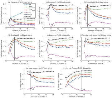
has Ktrue = [Kmax/2]clusters. Now for each value of K, generate 10,000 random clusterings and

calculate the average MI, NMImax, VI, RI and ARI between those clusterings to a fixed, random

2. Available online athttp://arxiv.org/abs/q-bio/0311039v2. 3. In their case 1, D′(Z,Y)is in fact not equal to H(Z|Y)/H(Y).

clustering chosen as the “true” clustering. The results for two combinations of(N,Ktrue)are given

in Fig. 1(a,b). It can be observed that the unadjusted measures such as the RI, MI and NMI (VI) monotonically increase (decreases) as K increases. Thus even by selecting totally at random, a 7-cluster solution would have a greater chance to outperform a 3-7-cluster solution, although there isn’t any difference in the clustering generation methodology. A corrected-for-chance measure, such as the ARI, on the other hand, has a baseline value always close to zero, and appears not to be biased in favor of any particular value of K. The same issue is observed with all other variants of the NMI (data not shown). Thus for this example, an adjusted-for-chance version of the MI is desirable.

5 10 15 20 0

0.2 0.4 0.6 0.8

Number of clusters K

Similarity/Distance value

(a) N=100 data points

← MI

← NMI

max

← VI

← ARI ← RI

K_true

10 20 30 40 50

0 0.2 0.4 0.6 0.8

Number of clusters K

Similarity/Distance value

(b) N=1000 data points

← MI

← _NMI

max

← VI

← ARI

← _RI

K true

5 10 15 20 0 0.2 0.4 0.6 0.8 1 1.2

Number of clusters K

Similarity/Distance value

(c) N=100 data points

← MI

← NMI

max

← VI

← ARI ← RI

10 20 30 40 50

0 0.2 0.4 0.6 0.8 1

Number of clusters K

Similarity/Distance value

(d) N=1000 data points

← MI

← NMI max ← VI

← ARI ← RI

Figure 1: (a,b) Average distance between sets of random clusterings to a “true” clustering (c,d) Average pairwise distance in a set of random clusterings. Error bars denote standard deviation.

2) Example 2 - Determining the number of clusters via consensus (ensemble) clustering: in an

era where a huge number of clustering algorithms exist, the consensus clustering idea (Monti et al., 2003; Strehl and Ghosh, 2002; Yu et al., 2007) has recently received increasing interest. Consensus clustering is not just another clustering algorithm: it rather provides a framework for unifying the knowledge obtained from other algorithms. Given a data set, consensus clustering employs one or several clustering algorithms to generate a set of clustering solutions on either the original data set or its perturbed versions. From these clustering solutions, consensus clustering aims to choose a robust and high quality representative clustering. Although the main objective of consensus clustering is to discover a high quality cluster structure, closer inspection of the set of clusterings obtained can often give valuable information about the appropriate number of clusters present. More specifically, we have empirically observed the following: in regard to the set of clusterings obtained, when the specified number of clusters coincides with the true number of clusters, this set has a tendency to be less diverse. This is an indication of the robustness of the obtained cluster structure. To quantify this diversity we have recently developed a novel index (Vinh and Epps, 2009), namely the consensus

index (CI), which is built upon a suitable clustering similarity measure. Given a value of K, suppose

we have generated a set of B clustering solutions

U

U

CI(

U

∑i<jAM(Ui,Uj)

B(B₋1)/2

where the agreement measure AM is a suitable clustering similarity index. Thus, the CI quantifies the average pairwise agreement in

U

that maximizes CI, that is, K∗=arg max_K=2...KmaxCI(

U

given N data points, randomly assign each data point into one of the K clusters with equal probability and check to ensure that the final clustering contains exactly K clusters. For each K, repeat this 200 times to create 200 random clusterings, then calculate the average values of the MI, VI, NMImax,

RI and ARI between all 19,900 clustering pairs. Typical experimental results are presented in Fig. 1(c,d). It can be observed that for a given data set, the average MI, NMI and RI (VI) values between random clusterings tend to increase (decrease) as the number of clusters increases, while the average value of the ARI is always close to zero. When the ratio of N/K is large, the average value for NMI

is reasonably close to zero, but grows as N/K becomes smaller. This is clearly an unwanted effect,

since a consensus index built upon the MI, NMI and VI would be biased in favour of a larger number of clusters. Thus in this situation, an adjusted-for-chance version of the MI is again important.

4.1 The Proposed Adjusted Measures

To correct the measures for randomness it is necessary to specify a model according to which ran-dom partitions are generated. Such a common model is the “permutation model” (Lancaster, 1969, p. 214), in which clusterings are generated randomly subject to having a fixed number of clusters and points in each clusters. Using this model, which was also adopted by Hubert and Arabie (1985) for the ARI, we have previously shown (Vinh et al., 2009) that the expected mutual information between two clusterings U and V is:

E{I(U,V)}= R

∑

C

∑

min(ai,bj)

∑

ni j

N log(

N.ni j aibj

) ai!bj!(N−ai)!(N−bj)!

N!ni j!(ai−ni j)!(bj−ni j)!(N−ai−bj+ni j)!

. (2)

As suggested by Hubert and Arabie (1985), the general form of a similarity index corrected for chance is given by:

Adjusted Index= Index− Expected Index

Max Index₋Expected Index, (3)

which is upper-bounded by 1 and equals 0 when the index equals its expected value. Having calcu-lated the expectation of the MI, we propose the adjusted form, which we call the adjusted mutual

information (AMI), for the normalized mutual information according to (3). For example, taking

the NMImaxwe have:

AMImax(U,V) =

NMImax(U,V)−E{NMImax(U,V)}

1₋E_{NMImax(U,V)}

= I(U,V)−E{I(U,V)}

max_{H(U),H(V)} −E_{I(U,V)}.

Similarly, other adjusted similarity measures are listed in Table 2. It can be seen that the adjusted-for-chance forms of the MI are all normalized in a stochastic sense. Specifically, the AMI equals 1 when the two clusterings are identical, and 0 when the MI between the two clusterings equals its expected value. The adjusted forms for the distance measures, listed in Table 2, are again the unit-complements of the corresponding adjusted similarity measures, for example, Admax=1−AMImax,

and are also normalized in a stochastic sense. Following the naming scheme that we have adopted throughout in this paper, we name Admaxthe adjusted information distance. It is noted that at this

stage, we have not been able to derive an analytical solution for the adjusted form for the normalized variation of information (djoint) measure. The derivation of the expected value for this measure

appears to be more involved observing that I(U,V)is present in both the numerator and denominator (H(U,V) =H(U) +H(V)₋I(U,V)). We repeat the experiments described in examples 1 and 2, this time with the adjusted version of the NMImax. Now it can be seen from Fig. 2 that just like the

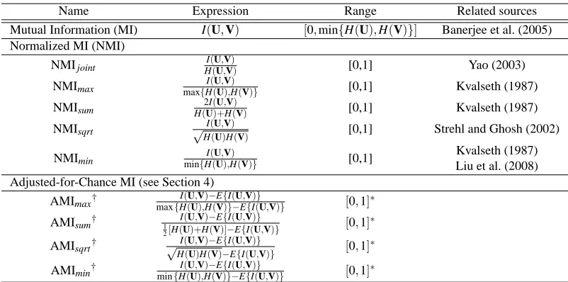
0 5 10 15 20 25 −0.03 −0.02 −0.01 0 0.01 0.02 0.03

Number of clusters K

Similarity/Distance value

(a) N=100 data points

← AMI max ← ARI

K true

0 20 40 60

−0.01 −0.005 0 0.005 0.01

Number of clusters K

Similarity/Distance value

(b) N=1000 data points

← AMI max ← ARI

K true

0 10 20 30

−0.03 −0.02 −0.01 0 0.01 0.02 0.03

Number of clusters K

Similarity/Distance value

(c) N=100 data points

← AMI max ← ARI

0 20 40 60

−0.01 −0.005 0 0.005 0.01

Number of clusters K

Similarity/Distance value

(d) N=1000 data points

← AMI max ← ARI

Figure 2: (a,b) Average distance between sets of random clusterings to a “true” clustering (c,d) Average pairwise distance in a set of random clusterings. Error bars denote standard deviation.

require the marginals of the contingency table to be fixed as per the assumption of the generalized hypergeometric model of randomness. Nevertheless, the adjusted measures still exhibit the desired behavior.

4.2 Properties of the Adjusted Measures

While admitting a constant baseline, the proposed adjusted-for-chance measures are, unfortunately, not proper metrics:

Theorem 6 The adjusted measures Admax,Adsum,Adsqrtand Adminare not metrics.

There is thus a trade-off between the metric property and correction for chance, and the user should decide which property is of higher priority. Fortunately, during our experiments with the AMI, we have observed that when the data contain a fairly large number of items as compared to the number of clusters, for example, N/K_≥100, then the expected mutual information is fairly close to zero, as can be seen in Fig. 1, suggesting scenarios where adjustment for chance is not of utmost necessity. The following results formalize this observation:

Theorem 7 Some upper bounds for the expected mutual information between two random

clus-terings U and V (on a data set of N data items, with R and C clusters respectively), under the hypergeometric distribution model of randomness are given by the followings:

E_{I(U,V)_{} ≤}

R

∑

i=1

C

∑

j=1

aibj

N2 log

N(ai−1)(bj−1)

(N₋1)aibj

+ N

aibj

≤log

N+RC₋R₋C

N₋1

. (4)

These bounds shed light on the large sample property of the adjusted measures. The following result trivially follows:

Corollary 1 Given R and C fixed, limN→∞E{I(U,V)}=0, and thus the adjusted measures tend

toward the normalized measures.

0.5978. As the maximum MI value is only log(10) =2.3, correction for chance is needed since the baseline is high. However, if the data size increases ten-fold to 1000 items, keeping the same num-ber of clusters and cluster distribution, the two upper bounds are 0.0764 and 0.0780 respectively, which can be considered small enough for many applications, therefore adjustment for chance might be omitted.

4.3 An Example Application

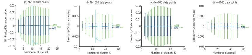
As per our analysis, adjustment for chance for information theoretic measures is mostly needed when the number of data items is relatively small compared to the number of clusters. One such prominent example is in microarray data analysis, where biological samples are clustered using gene expression data. Due to the high cost of preparing and collecting microarray data, each class, for example, of tumor, might contain only as few as several samples. In this section we demonstrate the use of the consensus index to estimate the number of clusters in microarray data. Eight synthetic and real microarray data sets are drawn from Monti et al. (2003), as detailed in Table 4 (see the original publication for preprocessing issues). A quick check upon the (higher) upper bound of the expected MI on these data sets suggests that correction for chance will be needed, for example, on the Leukemia data set, as K(=R=C)grows from 2 to 10, this upper bound grows from 0.03 to 1.16.

Simulated Data #Classes #Samples #Genes Real data #Classes #Samples #Genes

Gaussian3 3 60 600 Leukemia 3 38 999

Gaussian5 5 500 2 Novartis 4 103 1000

Simulated4 4 40 600 Lung cancer 4+ 197 1000

Simulated6 6-7 60 600 Normal tissues 13 90 1277

Table 4: Microarray data sets summary, source: Monti et al. (2003)

In Vinh and Epps (2009) we have shown that the CI, coupled with sub-sampling as the pertur-bation method, gives useful information on the appropriate number of clusters in microarray data. Herein, we experimented with random projection as the perturbation scheme. More specifically, the original data set was projected on a random set of 80% of the genes, and the K-means clustering algorithm was run with random initialization on the projected data set. For each value of K, 100 of such clustering solutions were created and the CI’s for 6 measures, namely RI, ARI, MI, VI, NMImaxand AMImaxwere calculated. Ideally we expect to see a strong global peak at the true

num-ber of cluster Ktrue. From Fig. 3(a) it can be observed that the unadjusted MI has a strong bias with

0 5 10 15 20 0 0.5 1 1.5 2 2.5

Number of clusters K

Similarity/Distance value

(a) Gaussian3, N=60 data points

K true MI NMI max AMI max VI ARI RI

0 5 10 15 20

0 0.2 0.4 0.6 0.8 1

Number of clusters K

Similarity/Distance value

(b) Gaussian5, N=500 data points

K true

0 5 10 15 20

0 0.2 0.4 0.6 0.8 1

Number of clusters K

Similarity/Distance value

(c) Simulated4, N=40 data points

K true

0 5 10 15 20

0 0.2 0.4 0.6 0.8 1

Number of clusters K

Similarity/Distance value

(d) Simulated6, N=60 data points

K

true

0 5 10 15 20

0 0.2 0.4 0.6 0.8 1

Number of clusters K

Similarity/Distance value

(e) Leukemia, N=38 data points

K true

0 5 10 15 20

0 0.2 0.4 0.6 0.8 1

Number of clusters K

Similarity/Distance value

(f) Norvatis multi−tissue, N=103 data points

K true

0 5 10 15 20

0 0.2 0.4 0.6 0.8 1

Number of clusters K

Similarity/Distance value

(g) Lung cancer, N=197 data points

K true

0 5 10 15 20

0 0.2 0.4 0.6 0.8 1

Number of clusters K

Similarity/Distance value

(h) Normal Tissues, N=90 data points

K true

Figure 3: Consensus Index on microarray data sets.

showing global or local peaks at or near the presumably true number of clusters as attributed by the respective authors calls for further investigation on both the biological side (re-verifying the number of clusters), and the CI side (the behaviour of the index with respect to the structure of the data set, for example, the data set might contain a hierarchy of clusters and thus the CI may exhibit local peaks corresponding to such structures).

5. Related Work

Meil˘a (2005) considered clustering comparison measures with respect to their alignment with the lattice of partitions. In addition to the metric property, she considered three more properties namely

additivity with respect to refinement, additivity with respect to the join and convex additivity, and

Wu et al. (2009) considered clustering comparison measures with respect to their sensitivity with class distribution. They showed that real life data can possess highly skewed class distributions, whereas some algorithms, such as K-means, tend to create balanced clusters. A good measure should therefore be sensitive to the difference in class distribution. To demonstrate this property, they used the example in Table 5, with a ground-truth clustering U having class sizes of [30, 2, 6, 10, 2], and two clustering solutions: V having cluster sizes of [10, 10, 10, 10, 10]; and V′ having cluster sizes of [29, 2, 6, 11, 2]. It is easily seen that V′ closely reflects the class structure in U, and thus should be judged closer to U than V. The authors showed that the unnormalized MI is a “defective measure”, in that it judges MI(U,V)>MI(U,V′), and suggested using the “normalized VI” (dsum). It can be shown that among the normalized and adjusted variants of the MI considered

in this paper, only the NMImin,Dmin,dminand Adminare defective measures in the above sense.

I U1 U2 U3 U4 U5 II U1 U2 U3 U4 U5

V1 10 0 0 0 0 V1′ 27 0 0 2 0

V2 10 0 0 0 0 V2′ 0 2 0 0 0

V3 10 0 0 0 0 V3′ 0 0 6 0 0

V4 0 0 0 10 0 V4′ 3 0 0 8 0

V5 0 2 6 0 2 V5′ 0 0 0 0 2

Table 5: Two clustering results

6. Conclusion

This paper has presented an organized study of information theoretic measures for clustering com-parison. We have shown that the normalized information distance (NID) and normalized variation of information (NVI) satisfy both the normalization and the metric properties. Between the two, the NID is preferable since the tighter upper bound of the MI used for normalization allows it to better use the [0,1] range. We highlighted the importance of correcting these measures for chance agreement, especially when the number of data points is relatively small compared with the number of clusters, for example, in the case of microarray data analysis. One of the theoretical advantages of the NID over the popular adjusted Rand index is that it can be used in the non-adjusted form (when N/K is large), thus enjoying the property of being a true metric in the space of clusterings.

We therefore advocate the NID as a “general purpose” measure for clustering validation, compar-ison and algorithm design, for it possesses concurrently several useful and important properties. Nevertheless, we note that for a particular application scenario, not always every desired property is needed concurrently, and therefore the user should prioritize the most important property. Our research systematically organizes and complements the current literature to help readers make more informed decisions.

Acknowledgments

We thank the Action Editor and the anonymous reviewers for their constructive comments. This work was partially supported by NICTA and the Australian Research Council.

Availability: Matlab code for computing the adjusted mutual information (AMI) is available

Appendix A. Proofs

Proof (Theorem 1) We only prove the triangle inequality as other parts are trivial. We first show

that

H(X_|Y)_≤H(X_|Z) +H(Z_|Y) (5)

holds true, since H(X_|Y)_≤H(X,Z_|Y) =H(X_|Z,Y)+H(Z_|Y)_≤H(X_|Z)+H(Z_|Y)(the last inequal-ity holds since conditioning always decreases entropy). We now prove the main theorem. Without loss of generality, assume that H(Y)_≤H(X), and therefore H(X_|Y)_≥H(Y_|X). The proof uses (5):

• Case 1: H(Z)_≤H(Y)

Dmax(X,Y) =H(X|Y)≤H(X|Z) +H(Z|Y)≤H(X|Z) +H(Y|Z) =Dmax(X,Z) +Dmax(Y,Z)

• Case 2: H(Y)<H(Z)_≤H(X)

Dmax(X,Y) =H(X|Y)≤H(X|Z) +H(Z|Y) =Dmax(X,Z) +Dmax(Y,Z)

• Case 3: H(X)<H(Z)

Dmax(X,Y) =H(X|Y)≤H(X|Z) +H(Z|Y)≤H(Z|X) +H(Z|Y) =Dmax(X,Z) +Dmax(Y,Z)

Proof (Theorem 3) We prove the triangle inequality. Without loss of generality, assume that H(X)_≥

H(Y), therefore H(X_|Y)_≥H(Y_|X)and NID(X,Y) =H(X_|Y)/H(X). The proof uses inequality (5) and simple algebra manipulations:

• Case 1: H(Z)_≤H(Y)_≤H(X)

NID(X,Y) =H(X|Y)

H(X) ≤

H(X_|Z) +H(Z_|Y)

H(X) ≤

H(X_|Z) +H(Y_|Z)

H(X) ≤

H(X_|Z)

H(X) +

H(Y_|Z)

H(Y)

• Case 2: H(Y)_≤H(Z)_≤H(X)

NID(X,Y) =H(X|Y)

H(X) ≤

H(X_|Z)

H(X) +

H(Z_|Y)

H(X) ≤

H(X_|Z)

H(X) +

H(Z_|Y)

H(Z) =NID(X,Z)+NID(Z,Y)

• Case 3: H(Z)>H(X)

NID(X,Y) =H(X|Y)

H(X) <

H(X_|Z) +H(Z_|Y)

H(X)

If the r.h.s_≤1 then adding H(Z)₋H(X)>0 to both its nominator and denominator will increase it:

r.h.s_≤H(X|Z) +H(Z|Y) +H(Z)−H(X)

H(X) +H(Z)₋H(X) =

H(Z_|X)

H(Z) +

H(Z_|Y)

therefore the triangle inequality holds. Otherwise if the r.h.s>1 then adding H(Z)₋H(X)>

0 to both its nominator and denominator as above will decrease it, but it will still be larger than 1. Therefore we also have:

NID(X,Y)_≤1<H(X|Z) +H(Z|Y) +H(Z)−H(X)

H(X) +H(Z)₋H(X) =NID(X,Z) +NID(Z,Y).

Proof (Theorem 4) Again only the triangle inequality proof is of interest. It is sufficient to prove

the following inequality:

H(X_|Y)

H(X,Y) ≤

H(X_|Z)

H(X,Z)+

H(Z_|Y)

H(Z,Y),

then swap X and Y to obtain another analogous inequality and add them together we have the triangle inequality. The proof uses inequality (5) and simple algebra manipulations:

H(X_|Y)

H(X,Y) =

H(X_|Y)

H(Y) +H(X_|Y) ≤

H(X_|Z) +H(Z_|Y)

H(Y) +H(X_|Z) +H(Z_|Y) =

H(X_|Z) +H(Z_|Y)

H(X_|Z) +H(Y,Z) =. . .

= H(X|Z)

H(X_|Z) +H(Y,Z)+

H(Z_|Y)

H(X_|Z) +H(Y,Z) ≤

H(X_|Z)

H(X_|Z) +H(Z)+

H(Z_|Y)

H(Y,Z)=

H(X_|Z)

H(X,Z)+

H(Z_|Y)

H(Z,Y).

Proof (Theorems 2 and 5) It is sufficient to point out a single counter example where the triangle

inequality is violated. Let X and Y be two independent random binary variables with probability

P(X =1) =P(X =0) =P(Y =1) =P(Y =0) =1/2, then Z= [X ;Y]is also a random variable with four discrete values. It is straightforward to verify that the triangle inequality is violated for all the mentioned distance measures, for example, Dmin(X,Y) =1<Dmin(X,Z) +Dmin(Y,Z) =0.

Proof (Theorem 6) For N=5, a counter example for the triangle inequality is the following three clusterings: U=_{U3U1U1U1U2},V={V2V2V3V1V2},X={X2X1X1X1X2}.

Similarly, for N =5+d (d _∈N+), a counter example for the triangle inequality is the fol-lowing three clusterings: U=_{U3U1U1U1U2U6U7. . .U5+d}, V={V2V2V3V1V2V6V7. . .V5+d}, X=

{X2X1X1X1X2X6X7. . .X5+d}.

Proof (Theorem 7) The following facts from the generalized hypergeometric distribution will be

useful:

E(ni j) =

∑

ni j

P

ai,bj

N , (6)

E(n2_{i j}) =

∑

n2_{i j}

P

ai(ai−1)bj(bj−1)

N(N₋1) +

aibj

N ,

where

P

ni j)( N−ni j ai−ni j)(

N−ai b j−ni j)

(N ai)(

N b j)

is the probability of encountering a contingency table M

model of randomness. Note that for the sake of notational simplicity we have dropped the lower and upper values of ni j which runs from max((ai+bj−N),0)to min(ai,bj)in the sums. From (6)

we have:

E(ni j) =

∑

ni j

P

aibj

N

∑

ni jN

aibj

P

aibj

N ,

therefore:∑_{ni j}ni jN

aibj

P

Q

ni jN

aibj

P

Q

as a discrete probability distribution on ni j. Applying Jensen’s inequality (E(f(x))≤ f(E(x))for

f concave) to the concave logarithm function yields:

∑

ni j

ni j

N log(

N.ni j

aibj

)

P

∑

aibj

N2 log(

N.ni j

aibj

)

Q

aibj

N2 log

EQ(

N.ni j

aibj

)

. (7)

Now, let us calculate EQ(N.n_aibi j_j ):

EQ(

N.ni j

aibj

) =

∑

ni j

N.ni j

aibj

Q

∑

ni j

N.ni j

aibj

ni jN

aibj

P

N2

a2_ib2_j

∑

2

i j

P

= N

2

a2_ib2_j

ai(ai−1)bj(bj−1)

N(N₋1) +

aibj

N

=N(ai−1)(bj−1) (N₋1)aibj

+ N

aibj

.

Substituting this expression into (7) yields:

∑

ni j

ni j

N log(

N.ni j

aibj

)

P

aibj

N2 log

N(ai−1)(bj−1)

(N₋1)aibj

+ N

aibj

.

Finally:

E_{I(U,V)_}= R

∑

i=1

C

∑

j=1

∑

ni j

N log(

N.ni j

aibj

)P(M_|ni j,a,b)≤ R

∑

i=1

C

∑

j=1

aibj

N2 log

N(ai−1)(bj−1)

(N₋1)aibj

+ N

aibj

.

(8) Note that∑_{i j}aibj/N2=1, continue applying Jensen’s inequality on (8) yields:

E_{I(U,V)_{} ≤}log

R

∑

i=1

C

∑

j=1

aibj

N2 (

N(ai−1)(bj−1)

(N₋1)aibj

+ N

aibj

)

!

=log

N+RC₋R₋C

N₋1

References

A. N. Albatineh, M. Niewiadomska-Bugaj, and D. Mihalko. On similarity indices and correction for chance agreement. Journal of Classification, 23(2):301–313, 2006.

A. Banerjee, I. S. Dhillon, J. Ghosh, and S. Sra. Clustering on the unit hypersphere using von mises-fisher distributions. J. Mach. Learn. Res., 6:1345–1382, 2005.

S. Ben-David, U. von Luxburg, and D. Pal. A sober look at clustering stability. In 19th Annual

Conference on Learning Theory (COLT 2006), pages 5–19, 2006.

M. Charikar, V. Guruswami, and A. Wirth. Clustering with qualitative information. In FOCS ’03:

Procs. IEEE Symposium on Foundations of Computer Science, 2003.

T. M. Cover and J. A. Thomas. Elements of Information Theory. Wiley, 1991.

B. E. Dom. An information-theoretic external cluster-validity measure. Technical report, Research Report RJ 10219, IBM, 2001.

X. Z. Fern and C. E. Brodley. Random projection for high dimensional data clustering: A cluster ensemble approach. In Procs. ICML’03, pages 186–193, 2003.

Z. He, X. Xu, and S. Deng. k-anmi: A mutual information based clustering algorithm for categorical data. Inf. Fusion, 9(2):223–233, 2008.

L. Hubert and P. Arabie. Comparing partitions. Journal of Classif., 2(1):193–218, 1985.

A. Kraskov, H. Stogbauer, R. G. Andrzejak, and P. Grassberger. Hierarchical clustering using mutual information. EPL (Europhysics Letters), 70(2):278–284, 2005.

T. O. Kvalseth. Entropy and correlation: Some comments. Systems, Man and Cybernetics, IEEE

Transactions on, 17(3):517–519, 1987.

H.O Lancaster. The chi-squared distribution. New York, 1969. John Wiley.

M. Li, X. Chen, X. Li, B. Ma, and P. Vit´anyi. The similarity metric. Information Theory, IEEE

Transactions on, 50(12):3250–3264, 2004.

Z. Liu, Z. Guo, and M. Tan. Constructing tumor progression pathways and biomarker discovery with fuzzy kernel kmeans and dna methylation data. Cancer Inform, 6:1–7, 2008.

P. Luo, H. Xiong, G. Zhan, J. Wu, and Z. Shi. Information-theoretic distance measures for clustering validation: Generalization and normalization. IEEE Trans. on Knowl. and Data Eng., 21(9): 1249–1262, 2009.

M. Meil˘a. Comparing clusterings by the variation of information. In COLT ’03, pages 173–187, 2003.

M. Meil˘a. Comparing clusterings: an axiomatic view. In ICML ’05: Proceedings of the 22nd

international conference on Machine learning, pages 577–584, 2005. ISBN 1-59593-180-5.

M. Meil˘a. Comparing clusterings—an information based distance. J. Multivar. Anal., 98(5):873– 895, 2007.

W. M. Rand. Objective criteria for the evaluation of clustering methods. Journal of the American

Statistical Association, 66(336):846–850, 1971.

O. Shamir and N. Tishby. Model selection and stability in k-means clustering. In 21th Annual

Conference on Learning Theory (COLT 2008), 2008.

V. Singh, L. Mukherjee, J. Peng, and J. Xu. Ensemble clustering using semidefinite programming with applications. Mach. Learn., 2009. doi: 10.1007/s10994-009-5158-y.

D. Steinley. Properties of the Hubert-Arabie adjusted Rand index. Psychol Methods, 9(3):386–96, 2004.

A. Strehl and J. Ghosh. Cluster ensembles - a knowledge reuse framework for combining multiple partitions. Journal of Machine Learning Research, 3:583–617, 2002.

K. Tumer and A.K. Agogino. Ensemble clustering with voting active clusters. Pattern Recognition

Letters, 29(14):1947–1953, 2008.

N. X. Vinh and J. Epps. A novel approach for automatic number of clusters detection in microarray data based on consensus clustering. In BIBE’09: Procs. IEEE Int. Conf. on BioInformatics and

BioEngineering, 2009.

N. X. Vinh, J. Epps, and J. Bailey. Information theoretic measures for clusterings comparison: Is a correction for chance necessary? In ICML ’09, 2009.

M. Warrens. On similarity coefficients for 2x2 tables and correction for chance. Psychometrika, 73 (3):487–502, 2008.

J. Wu, H. Xiong, and J. Chen. Adapting the right measures for k-means clustering. In KDD ’09, 2009.

Y. Y. Yao. Information-theoretic measures for knowledge discovery and data mining. In Entropy

Measures, Maximum Entropy Principle and Emerging Applications, pages 115–136. Karmeshu

(ed.), Springer, 2003.