NEUROSVM: An Architecture to Reduce the Effect of the Choice of
Kernel on the Performance of SVM
Pradip Ghanty [email protected]
Praxis Softek Solutions Pvt. Ltd.
Module 616, SDF Building, Sector V, Salt Lake City Calcutta - 700 091, India
Samrat Paul [email protected]
IBM India Pvt. Ltd.
DLF IT Park, 4thFloor, Tower C, New Town Rajarhut Calcutta - 700 156, India
Nikhil R. Pal [email protected]
Electronics and Communication Sciences Unit Indian Statistical Institute
203, B. T. Road
Calcutta - 700 108, India
Editor: Yoshua Bengio
Abstract
In this paper we propose a new multilayer classifier architecture. The proposed hybrid architecture has two cascaded modules: feature extraction module and classification module. In the feature extraction module we use the multilayered perceptron (MLP) neural networks, although other tools such as radial basis function (RBF) networks can be used. In the classification module we use sup-port vector machines (SVMs)—here also other tool such as MLP or RBF can be used. The feature extraction module has several sub-modules each of which is expected to extract features capturing the discriminating characteristics of different areas of the input space. The classification module classifies the data based on the extracted features. The resultant architecture with MLP in feature extraction module and SVM in classification module is called NEUROSVM. The NEUROSVM is tested on twelve benchmark data sets and the performance of the NEUROSVM is found to be better than both MLP and SVM. We also compare the performance of proposed architecture with that of two ensemble methods: majority voting and averaging. Here also the NEUROSVM is found to perform better than these two ensemble methods. Further we explore the use of MLP and RBF in the classification module of the proposed architecture. The most attractive feature of NEUROSVM is that it practically eliminates the severe dependency of SVM on the choice of kernel. This has been verified with respect to both linear and non-linear kernels. We have also demonstrated that for the feature extraction module, the full training of MLPs is not needed.
Keywords: feature extraction, neural networks (NNs), support vector machines (SVMs), hybrid
1. Introduction
A classifier designed from a data set X={xi|i=1,2, . . . ,N,xi∈ℜp}, whereℜpis the p dimensional real space, can be defined as a function G :ℜp→Nc. Here Nc={y∈ℜc: yk∈ {0,1}∀k,
c
∑
k=1
yk=1}
is the set of label vectors and c is the number of classes. For any input vector x∈ℜp, G(x)is a vector in c dimension with only one component as 1 and all others 0. In this paper our primary objective is to find a good G combining neural networks (NNs) and support vector machines (SVMs).
In machine learning literature NN and SVM are two widely used classifiers. NNs have been developed for many years and been used in various applications (Haykin, 1999; Pal et al., 2006). The SVM (Vapnik, 1995) is a classification and regression tool. It is comparatively a new family of learning tools including training algorithms for optimal margin classifiers (Boser et al., 1992) and support vector networks (Cortes and Vapnik, 1995). In SVM the input data are often transformed into a high dimensional space using some kernel functions. A linear separating hyper plane with the maximal margin between the closest positive and closest negative samples in the mapped space is found. The SVM works by solving a quadratic optimization problem that minimizes a sum of two terms. The first term is related with the reciprocal of norm of weight vector associated with the hyper plane and the second term is related to the sum of classification error. The SVM is a very active topic of research (von Luxburg et al., 2004; Adankon and Cheriet, 2007) and it has been successfully applied to many areas including handwritten digit recognition (Vapnik, 1995), object recognition (Pontil and Verri, 1998), protein structure prediction (Nguyen and Rajapakse, 2003) and texture classification (Kim et al., 2002). But there are some computational difficulties associated with using SVM. One of them is the required memory, which grows very quickly with the size of the training data since the SVM algorithm involves solving a large quadratic programming problem where every training data point forms a constraint. This is a constraint on the application of SVM to very large data sets. More importantly, the performance of SVM is significantly dependent on the choice of kernel. Needless to say that for non-linearly separable data, the performance of linear and nonlinear SVM also differs significantly.
Use of an ensemble of classifiers is a popular approach to improve the classification perfor-mance. Many ensemble methods are used by researchers to report the improvement in performance over single classifier (Hansen, 1999; Maqsood et al., 2004; Chawla et al., 2004). An ensemble of classifiers can be constructed using both homogeneous and heterogeneous classifiers (Hansen, 1999; Prevost et al., 2003; Garcia-Pedrajas et al., 2005). An ensemble of neural networks is often used for pattern classification problems (Garcia-Pedrajas et al., 2005; Islam et al., 2003) including face recognition (Melin et al., 2005), weather forecasting (Maqsood et al., 2004), protein secondary structure prediction (Guimaraes et al., 2003). Different approaches for constructing ensemble of neural networks have been suggested in the literatures (Wu et al., 2001; Zhou et al., 2002; Windeatt, 2006). In this paper for the purpose of comparison we have considered two ensemble methods for neural networks, one uses the average output of the ensemble of networks while the other one makes the ensemble vote on a classification task.
In this context, the ensemble method of Garcia-Pedrajas et al. (2007) needs a special attention as this method also uses a multilayer perceptron network for feature extraction and hence one may get a false impression that this method and our proposed method are quite similar.
Like AdaBoost the first baseline classifier is trained using the original training data while each of the subsequent classifiers is trained using a projected data set created using the hidden output of a trained MLP. The second baseline classifier uses data projected through the hidden layer of a projection network (MLP here). The projection network is an MLP network with number of hidden nodes equal to the number of inputs in the original training data and it is trained using only that subset of the training data which are not classified correctly by the first baseline classifier. The projection network (again an MLP with number of hidden nodes equal to the number of inputs in the original data) for the third baseline classifier is trained using the original data points whose projected versions are wrongly classified by the second baseline classifier. The process is repeated to generate a large number of baseline classifiers.
Note that, our proposed method falls in the category of hybrid system. There have been several attempts to combine different machine learning tools to develop efficient hybrid systems for pattern classification problems (Huang and LeCun, 2006; Happel and Murre, 1994; Vincent and Bengio, 2000; Mitra et al., 2006, 2005). To design a hybrid system different combination of classifiers is used including neural network-SVM (Mitra et al., 2005, 2006; Vincent and Bengio, 2000), convolution network-SVM (Huang and LeCun, 2006). Neural networks and support vector machines are used to design a hybrid system for text classification in Mitra et al. (2005) and Lidar detection of underwater objects in Mitra et al. (2006). Mitra et al. (2005) proposed a hybrid system called neuro-SVM which takes the component wise product of the outputs of a cascaded-SVM classifier and a recurrent neural network, and applies a set of heuristic rules to decide on the class. In the work of Mitra et al. (2006), after preprocessing Lidar signal is modeled using a polynomial as well as a linear predictor. The optimal coefficients of the polynomial are used as inputs to train a RBF, while coefficients of the linear predictor are used to train an MLP. The products of the corresponding components of the output vectors from the two networks are used as input to a cascaded-SVM classifier. Huang and LeCun (2006) presented a hybrid system for object recognition that uses the outputs of the last hidden layer of a convolution network to train a SVM with Gaussian kernel. The convolution network is generally used for computer vision problems. A convolution network has several hidden layers alternately consisting of convolution layer and sub-sampling layer. In a convolution network, the successive layers are designed to learn progressively higher-level features until the last layer, which produces categories.
There have been a number of attempts to develop modular networks to solve complex prob-lems efficiently (Ronco and Gawthrop, 1995; Bottou and Gallinari, 1991). The basic philosophy of developing a modular network is to divide the task into a number of, preferably, meaningful subtasks, and then design one module for each subtask. Finally one needs to devise a mechanism to integrate these modules—this will dictate how different modules interact and lead to the final output. Sometimes the knowledge of the problem domain can be used to find the subtasks, but often clustering is used for this purpose. For example in Pal et al. (2003) a self organized map (SOM) is used to find natural clusters (subtasks) in the data and then for each cluster a separate network is trained. A given input is routed to the appropriate MLP module using the SOM. Jenkins and Yuhas (1993) have presented a simple solution to the truck backer-upper problem by decomposing it into subtasks. Then all subtasks are realized in parallel (that is, off line) to obtain the final two-layer feed-forward network, which is used to control the truck. Although our proposed architecture uses several modules, this is not designed following the usual principle of modular network.
feature extraction module (FM), because outputs of this module can be used as inputs to any other classifier. This new set of features is used in the next module, termed as the classification module (CM). In the classification module we have used SVM with different kernel functions. Instead of SVM, one can use any other classifier also. We also consider the MLP and RBF neural networks in the CM of our proposed architecture. To further demonstrate the effectiveness of NEUROSVM we compare it with two other ensemble methods: majority voting and averaging. We demonstrate the effect of the kernel on SVM and NEUROSVM.
Our proposed method is neither an ensemble method nor has any relation to boosting. There is only one classifier. The classifier uses features extracted from the hidden nodes of several trained networks where typically the number of hidden nodes in a network is smaller than input dimension. Each network used for feature extraction is trained using the same data and each network sees the entire input space as represented through the training data. Thus typically to get improved performance we need fewer feature extraction networks than that would be needed by the ensemble type methods.
2. Methods
The section is arranged as follows. First, we provide a brief description of neural networks for the sake of completeness. Next, we give a brief description of the support vector machine (SVM) classifier and how several binary SVMs can be combined to solve a multiclass problem. Then we explain two popular existing ensemble methods that will be used for comparison. This is followed by a detailed discussion of the proposed method.
2.1 MLP and RBF Neural Networks
The two most widely used neural networks for pattern recognition are multilayer perceptron (MLP) and radial basis function (RBF) networks (Haykin, 1999). We have used the back-propagation algorithm for training MLP networks with single hidden layer.
The RBF network consists of exactly three layers: input layer, basis function layer and output layer. Unlike MLP, the activation functions of the hidden nodes are not of sigmoidal type, rather each hidden node represents a radial basis function. The transformation from the input space to the hidden space is nonlinear but each node in the output layer computes just the weighted sum of the outputs of the previous layer, that is, each output layer node makes a linear transformation. The learning of RBF network is usually performed in two phases. An unsupervised learning method is applied to estimate the basis function parameters. Then a supervised learning method, such as gradient descent or least square error estimate, is applied to tune the network weights between the hidden layer and the output layer. However, the parameters of the basis functions can also be tuned using gradient descent technique. Here we have used the MATLAB implementation of RBF network.
2.2 Support Vector Machines (SVMs)
Given a training set (X,Y), xi ∈X, xi ∈ℜp and y
i ∈Y , the class label associated with xi;
yi∈ {−1,+1}, the learning problem for SVMs is to find the weight vector w and bias b such that they satisfy the constraints:
xi.w+b>+1 for yi= +1 (1)
xi.w+b6−1 for yi=−1 (2)
and the weight vector w minimizes the cost function
Φ(w) =1 2w
Tw.
The constraints written in Equations (1)-(2) can be combined as
yi(xi.w+b)>+1∀i.
If the training points are not linearly separable, then there is no hyperplane that separates them into positive and negative classes. In this case, the problem is reformulated considering the slack variablesξi>0; i=1,2, . . . ,N. For most xi, ξi=0. The constraints are now modified as follows:
xi.w+b>+1−ξi for yi= +1 (3)
xi.w+b6−1+ξi for yi=−1 (4)
ξi>0,∀i. (5)
The SVM then finds w, minimizing
Φ(w,ξ) =1 2w
Tw+C
∑
Ni=1
ξi
subject to constraints as in Equations (3)-(5). The constant C is termed as a regularization parameter as it controls the trade off between the complexity of the machine and the number of misclassifica-tions.
Typically, when the training points are not linearly separable, a nonlinear mappingϕis used to map the training data fromℜp to some higher dimensional feature space H, with a hope that the data may be linearly separable in H. The mapping is implicitly realized using a kernel function.
Two kernels that are popular for non-linear SVMs are:
1. Polynomial of degree d: K(x,xi) = (sx.xi+1)d, where s is the scaling coefficient of the dot product.
2. Radial Basis Function (RBF): K(x,xi) =e−γkx−xik2,γ>0.
In this study, we shall extensively use the RBF kernel with a wide range ofγ. We shall also demon-strate the utility of the proposed method with polynomial kernel.
2.3 SVM for Multiclass Problems
The preceding SVM formulation is for two class problems. Multiclass SVMs are generally realized using several two class SVMs. We use the One versus One (OVO) method (Nguyen and Rajapakse, 2003; Weston and Watkins, 1999). Let us assume that we have a c class problem. In this method we construct one binary classifier for every pair of distinct classes. So we get c×(c−1)/2 binary
classifiers for a c class problem. In the training data, suppose kisamples are from class i, N= c
∑
i=1ki. For the class pair(i,j), a binary classifier Ci jis trained using kiand kjdata points from class i and j. An unknown sample x is then classified by each of the c×(c−1)/2 different classifiers. If classifier Ci j classifies x as class i then the vote for class i for sample x is increased by one. Otherwise, vote for class j for sample x is increased by one. In this way for sample x, the votes for all c classes are calculated using the output of all c×(c−1)/2 classifiers. After that we assign x to class l, if class l has the largest number of votes for x. Ties are randomly resolved.
2.4 Ensemble Methods: Majority Voting and Averaging
Different methods of classifier fusion are available in the literature (Maqsood et al., 2004; Ko et al., 2007; Brown et al., 2005; Tang et al., 2006; Kuncheva and Whitaker, 2003; Windeatt, 2006; Islam et al., 2003), of which the majority voting scheme is probably the most popular method (Stepenosky et al., 2006). In this method, the final class is determined by the maximum number of votes counted among all the classifiers fused. Let us consider a c class problem and let m be the number of classifiers to be fused. For an unknown sample x, vote for class j, vj,(j=1,2, . . . ,c)is computed from the ensemble of classifiers Ci,(i=1,2, ...,m). If Ci,(i=1,2, ...,m)assigns sample x to class
j then vjis incremented by 1. Note that, initially vote for every class is initialized to 0; that is, vj= 0,(j=1,2, ...,c). The final class determination by the ensemble for sample x is k, if vk=
c max
j=1{vj}.
Averaging also is a simple but effective method and is used in many classification problems (Guimaraes et al., 2003; Naftaly et al., 1997). In this method, the final class is determined by the average of continuous outputs of all classifiers (here MLPs) fused. For an unknown sample x, let the output for class j(j=1,2, ...,c)from classifier Ci,(i=1,2, ...,m)be oi j. Then the output from
the ensemble classifier is obtained as Oj= m1 m
∑
i=1
oi j, j=1,2, . . . ,c. The final class assignment by
the ensemble to x is k, if Ok= c max
j=1{Oj}.
2.5 Proposed NEUROSVM Classifier
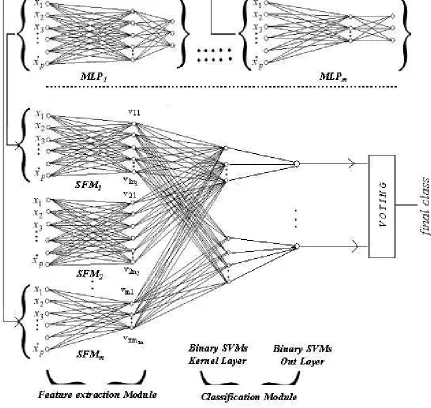
The proposed multilayer architecture can be thought of as a combination of two types of modules: feature extraction module (FM) and classification module (CM). The FM consists of a number of sub-modules SFMi, i=1,2, . . . ,m. Each sub-module SFMi takes the same p dimensional data x= (x1,x2, . . . ,xp)T as input and produces ni dimensional output vectors vi = (vi1,vi2, . . . ,vini)
T.
Thus n= ∑m i=1
input to the classification module. z= v1 v2 .. . vm
∈ℜn1+n2+...+nm (6)
and
v1 = (v11,v12, . . . ,v1n1)
T , v2 = (v21,v22, . . . ,v2n2)
T
, (7)
.. .
vm = (vm1,vm2, . . . ,vmnm)
T.
In general, different SFMi can use different methods of feature extractions or they can use the same principle for feature extraction. Similarly, the classification module can use any principle like neurocomputing, support vector machines and so on.
In this investigation, the sub-modules SFMis are derived from multilayer perceptron networks, while the classification module consists of support vector machines. And, hence, we call the result-ing architecture NEUROSVM.
In order to constitute the ith sub-module SFMi, we consider an MLP with just one hidden layer, with architecture(p,ni,c), where p is the input dimension, niis the number of nodes in the hidden layer and c is the number of classes. Note that, although the number of input and output nodes in each MLP remains the same, the number of nodes in the hidden layer could be different for different MLPs. Each MLP is then trained using the training data X={xi; i=1,2, . . . ,N} ⊂ℜp, Y ={yi; i=1,2, . . . ,N} ⊂ℜcwhere yiis the target output corresponding to xi.
Once each network is trained, the output of the hidden layer can be taken as the extracted features. These features capture characteristics of the data that can discriminate between classes; hence using these features we can do the classification job using just a single layer network.
Note that, instead of MLP, we can use RBF also in the feature extraction module. In Figure 1, the top panel has m different trained MLPs labeled as MLP1,MLP2, . . . ,MLPm. After the train-ing, we remove the output layer and its associated connections from each of the MLPs and then the truncated two-layer sub-networks are taken as feature extraction sub-modules. The subnets SFM1,SFM2, . . . ,SFMm in the lower panel of the NEUROSVM are constructed from the trained MLPs in the upper panel. The first two layers of MLPiconstitute SFMi,i=1,2, . . . ,m.
As depicted in the lower panel of Figure 1, the output from the m sub-modules, taken together constitutes the input to the classification module. Here we consider SVMs for classification, but other classifiers such as neural networks (MLP or RBF network) can also be used. Note that, each sub-module receives the same input x= (x1,x2, . . . ,xp)T.
In the present case the CM has two layers. The first layer, as shown in Figure 1, is the SVM kernel layer where each node is associated to a mapped training sample zi(it is the output from an FM that represents a support vector) and it computes the kernel output K(z,zi)on a mapped input z, while the other layer is the output layer.
Figure 1: The proposed NEUROSVM classifier
2.6 Advantages of the Proposed Method
1. Typically, due to the local minima problem of MLP training and its dependence on initial-ization, different MLPs may learn different areas of the input space better. Hence when we combine the output of the hidden layer of different networks to generate new features, the learning task becomes simpler to the CM. This is true irrespective of whether the CM is a neural network or SVM.
2. The extracted features result in simpler classification boundaries because a single layer net-work can classify the new data (consider a two layer netnet-work consisting of the hidden and output layers of an MLP). This also makes the learning task of the CM simpler.
3. For high dimensional data, typically the number of nodes in the hidden layer is much smaller than the number of the input nodes and one does not need many feature extraction sub-modules (SFMs). Hence, the dimensionality of the input for the CM can be reduced com-pared to the original dimension of the input. This makes simpler error surface, faster learning and allows us to do more experiments, if CM is a neural network.
4. This is not an ensemble method but it makes fusion of salient characteristics of the input space as extracted/learnt by different feature extraction networks. It can at least be viewed as an implicit fusion of multiple classifiers, and hence improvement in performance is expected.
5. For large data sets, it may not be necessary to make full training of the MLPs for constructing the SFMis, because the objective of the MLPs here is to capture the inherent attributes of the data by the FM.
For low dimensional data sets or simpler data sets this method may not have much advantage be-cause then n (dimension of input to the CM) can be more than p (original dimension of the input) and different SFMs may capture the same attributes of the data resulting in not much of benefits. Note that, the advantages mentioned in 2 and 3 are also applicable to MLPs.
3. Experiments
The section is arranged as follows. First we have listed the selected data sets to validate our proposed method. Then experimental setup is described. Next, the experimental results are presented. Finally, a control experiment to justify one of the advantages of the proposed method is demonstrated.
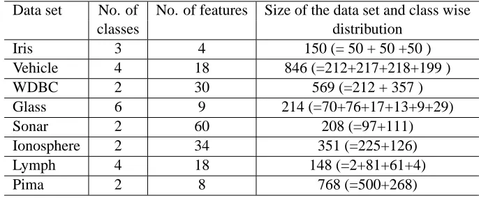
3.1 Data Sets
four data sets in Group B, benchmark results with different classifiers are available along with the training-test partition. Hence we have used the same training-test partition here and report the error on the fixed test set. Table 1 and Table 2 summarize the Group A and Group B data sets respectively.
Data set No. of No. of features Size of the data set and class wise
classes distribution
Iris 3 4 150 (= 50 + 50 +50 )
Vehicle 4 18 846 (=212+217+218+199 )
WDBC 2 30 569 (=212 + 357 )
Glass 6 9 214 (=70+76+17+13+9+29)
Sonar 2 60 208 (=97+111)
Ionosphere 2 34 351 (=225+126)
Lymph 4 18 148 (=2+81+61+4)
Pima 2 8 768 (=500+268)
Table 1: Group A data sets
Data set No. of No. of Training data Test data
classes features Size Class distribution Size Class distribution 780, 779, 780, 719 363, 364, 364, 336 Pendigits 10 16 7494 780, 720, 720, 778 3498 364, 335, 336, 364
719, 719 336, 336
Img. Seg. 7 18 210 30 in each class 2100 300 in each class
104, 68, 108, 47 1429, 635, 1250, 579
Sat. Img. 6 4 500 58, 115 5935 649, 1393
376, 389, 380, 389 178, 182, 177, 183 Optdigits 10 64 3823 387, 376, 377, 387 1797 181, 182, 181, 179
380, 382 174, 180
Table 2: Group B data sets
3.2 Experimental Setup
In this subsection we describe the selection method for hyper parameters of MLP and SVM classi-fiers. To select the optimal architecture for an MLP, Andersen and Martinezr (1999) used ten-fold cross-validation experiments. Adankon and Cheriet (2007) discussed another scheme for SVM model selection. Here we have used ten-fold cross-validation experiments for MLP architecture selection as well as for selection of SVM kernel parameters. For Group B data sets training-test partitions are fixed and hence we have used ten-fold cross-validation on the training set to select the hyper parameters of classifiers. For Group A data sets, as mentioned earlier, the performances are reported based on ten-fold cross-validation. So, we perform double blind ten-fold cross-validation experiments to select hyper parameters of classifiers for Group A data sets.
Based on validation error we choose m architectures for each of the ten folds for Group A data sets and m architectures for each of the Group B data sets for NEUROSVM.
In a similar manner the regularization parameter C and spreadγof RBF kernels of SVMs are chosen based on ten-fold cross-validation experiments. We have experimented with nc choices of
C and ngchoices ofγ. So, we have used nc×ngsets of choice of parameters. For each choice, the ten-fold cross-validation experiments are conducted. Here we also select the(C,γ)pair that leads to the minimum average validation error. In this investigation nc=12 and ng=15 are used resulting in a total of 180 pairs of parameters.
We have also used ten-fold cross-validation to find the sub-modules for NEUROSVM. The hyper parameters of SVMs in the classification module of NEUROSVM are also estimated through fold cross-validation experiments. Note, for Group A data sets we have used double blind ten-fold cross-validation. We have selected m (=5) SFMs. Hence using the m SFMs we can generate 2m−1 different feature subsets combinations. In our case it is 25−1=31. Then for each of the 31 combinations with all 180 pairs of(C,γ) we have conducted the ten-fold cross-validation experiments on training set(s). We have obtained the best(C,γ)for each of the 31 combinations. Then the best combination is chosen based on the minimum average validation error over all 31 combinations. Finally using the best combination and corresponding(C,γ)pair the performance of NEUROSVM is reported.
We have performed statistical tests (Dietterich, 1998) to compare the proposed algorithms with that of standard algorithms. For Group A data sets where cross-validation is performed, we have applied the ten-fold cross-validation paired t-test with 9 degrees of freedom and 95% significance level. For the four data sets of Group B where a single test set is employed, we have constructed McNemar test with 1 degree of freedom and 95% significance level. The formulations of these tests are as follows.
3.2.1 K-FOLDCROSS-VALIDATIONPAIRED T-TEST(DIETTERICH, 1998)
Consider two classifier models, D1 and D2, and a data set X . The data set is split into K parts of approximately equal sizes, and each part is used in turn for testing of a classifier built on the pooled remaining K−1 parts. Classifiers D1and D2are trained on the training set and tested on the test set. Denote the observed test accuracies as P1 and P2, respectively. This process is repeated K times and test accuracies are tagged with superscript(i),i=1,2, . . . ,K. Thus a set of K differences is obtained, P(1)=P1(1)−P2(1)to P(K)=P1(K)−P2(K). Under the null hypothesis (H0: equal accuracies), the following statistic has a t-distribution with K−1 degrees of freedom
t= P
√
K s
K
∑
i=1
(P(i)−P)2/(K−1) ,
where P= (1/K) ∑K i=1
P(i). If the calculated t is greater than the tabulated value for chosen level of
3.2.2 MCNEMARTEST(DIETTERICH, 1998)
As done before consider two classifiers D1 and D2. Let us define the following: N00= number of samples which both D1and D2 classify incorrectly, N01 = number of samples which D1 classifies incorrectly but D2 classifies correctly, N10 = number of samples which D1 classifies correctly but
D2classifies incorrectly and N11= number of samples which both D1and D2classify correctly. Let,
N=N00+N01+N10+N11be the total number of samples in the test set. The null hypothesis, H0, is that there is no difference between the accuracies of the two classifiers. If the null hypothesis is correct, then the expected counts for N01 and N10are 12(N01+N10). The discrepancy between the expected and the observed counts is measured by the following statistic
χ2=(|N01−N10| −1)
N01+N10 ,
which is approximately distributed asχ2with 1 degree of freedom. To carry out the test we simply calculateχ2 and compare it with the tabulatedχ2value for a given level of significance, say, 0.05 (in our case).
We have performed all experiments using two Sun Blade 2500 with dual processors. The svm learn and svm classify modules for binary SVMs training and classification are used from SV Mlight (Joachims, 2002) software. For the RBF neural network MATLAB toolbox is used. All other programs are written in c.
3.3 Experimental Results
In this subsection first we list the selected hyper parameters of MLP and SVM by cross-validation experiments. Next selection of sub-modules and hyper parameters of NEUROSVM is discussed. The performance comparison of NEUROSVM with the baseline classifiers and standard ensemble methods is presented. Finally, we present the performance of other variants of NEUROSVM and compare it with the baseline classifiers as well as ensemble methods.
3.3.1 SELECTION OFHYPERPARAMETERS FORMLPS TOCONSTRUCT THEFM
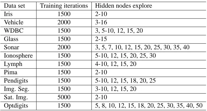
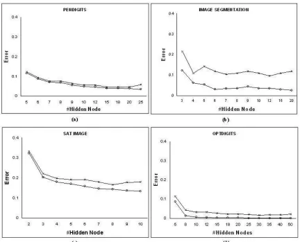
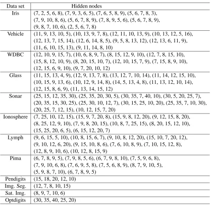
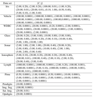
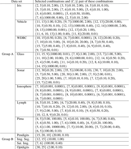
For Group A data set we use double blind ten-fold cross-validation. The partitioning of data for Group A data sets is explained in Appendix A. For each of the outer level cross validation loop, finding the optimal number of hidden nodes and computation of the test error are explained in the procedure RunMLP in Appendix B. The initial weights of the MLPs are chosen randomly in [-0.5, +0.5] and the learning rate used to train the MLPs is 0.60. The number of iterations used to train the networks for different data sets are chosen based on a few trial experiments. For each data set, a set of choices on the number of hidden nodes is used to train the MLPs. In Table 3, number of iterations and number of hidden nodes that are used to train the MLPs for the twelve data sets are listed. We have decided to use m=5 neural networks for feature extraction modules and hence for each fold, we have to select a set of five hidden nodes to train five MLPs.
A. Suppose, we have trained MLPs with M different architectures, that is, with M different choices of hidden nodes. Then for each of the outer level fold, we shall have M different hidden nodes each associated with an average validation error. Now we order these M hidden nodes in ascending order of the associated validation error. Then select the top five hidden nodes from this ordered list. These five different choices of hidden nodes will be used to train five MLPs for feature extraction for that particular fold. For each data set, in Table 4, we depict the list of selected hidden nodes for each fold (outer level). As an example, for the IRIS data for the first fold (outer level), the selected hidden nodes are (7, 2, 5, 6, 8). This means that for the first fold (outer level) we got the least validation error with 7 hidden nodes; the next smaller validation error is obtained with 2 hidden nodes and so on.
Since the first element of this set of five resulted in the smallest validation error, we use this choice of hidden nodes to train MLPs when we report the performance of the MLP networks as classifiers. For each data set in Group B, since the training and test partitions are fixed, we have only one outer loop and hence only one set with five choices of hidden nodes as shown in Table 4. We follow the same protocol as that of Group A data sets to choose the number of hidden nodes for computing the performance of MLP networks.
Data set Training iterations Hidden nodes explore
Iris 1500 2-10
Vehicle 2000 3-16
WDBC 1500 3, 5-10, 12, 15, 20
Glass 1500 2-15
Sonar 2000 3, 5, 7, 10, 12, 15, 20, 25, 30, 35, 40 Ionosphere 1500 5-10, 12, 15, 20, 25, 30
Lymph 1500 4-10, 12, 15, 20
Pima 1500 2-10
Pendigits 1500 5-10, 12, 15, 18, 20, 25
Img. Seg. 1500 3-10, 12, 15, 20
Sat. Img. 5000 2-10
Optdigits 1500 5, 8, 10, 12, 15, 18, 20, 25, 30, 35, 40, 50
Table 3: List of explore hidden nodes and number of iterations for MLP for the twelve data sets
3.3.2 SELECTION OFHYPERPARAMETERS FORSVMS
In this section we consider the problem of selecting hyper parameters for a regular SVM that we shall use as benchmark in experiments for the purpose of comparison with NEUROSVM. To select the regularization parameter C and spreadγfor RBF kernel of SVM classifiers we have tried a wide range of C andγ. In this experiment we have used 12 different values of C and 15 different values of
the obtained optimal set of parameters is in Table 5. The results reported for SVMs correspond to these choices.
Data set Hidden nodes
Iris (7, 2, 5, 6, 8), (7, 9, 3, 6, 5), (7, 6, 5, 8, 9), (5, 6, 7, 8, 3), (7, 9, 10, 8, 6), (5, 6, 7, 8, 9), (7, 8, 9, 5, 6), (5, 6, 7, 8, 9), (9, 8, 7, 10, 6), (2, 5, 6, 7, 8)
Vehicle (11, 9, 13, 10, 5), (10, 13, 9, 7, 8), (12, 11, 10, 13, 9), (10, 13, 12, 5, 16), (12, 13, 7, 15, 14), (12, 6, 14, 8, 5), (9, 5, 8, 13, 12), (12, 13, 6, 11, 9), (11, 6, 10, 15, 13), (9, 11, 14, 8, 10)
WDBC (12, 10, 9, 15, 7), (10, 6, 8, 9, 7), (8, 15, 12, 9, 10), (12, 7, 8, 15, 10), (15, 8, 12, 10, 9), (8, 20, 15, 10, 7), (12, 10, 15, 7, 9), (7, 15, 8, 9, 10), (12, 15, 6, 9, 10), (9, 7, 20, 10, 12)
Glass (11, 15, 13, 4, 9), (12, 9, 13, 7, 8), (13, 12, 7, 10, 14), (11, 14, 12, 15, 10), (10, 15, 9, 13, 6), (10, 12, 9, 14, 8), (14, 5, 13, 4, 8), (11, 13, 12, 10, 14), (12, 15, 8, 6, 9), (11, 13, 14, 15, 12)
Sonar (25, 15, 12, 35, 30), (25, 35, 20, 30, 5), (30, 35, 7, 40, 10), (30, 5, 20, 25, 7), (20, 35, 15, 30, 25), (25, 30, 10, 12, 7), (30, 15, 25, 10, 20), (25, 35, 7, 10, 30), (20, 25, 7, 12, 15), (10, 12, 15, 7, 20)
Ionosphere (7, 25, 10, 12, 15), (15, 9, 7, 20, 8), (15, 9, 8, 12, 20), (9, 12, 15, 8, 20), (8, 25, 12, 9, 10), (7, 9, 8, 20, 15), (10, 8, 7, 25, 15), (8, 20, 15, 12, 10), (15, 25, 20, 6, 5), (6, 15, 12, 20, 7)
Lymph (9, 6, 15, 5, 10), (10, 8, 15, 6, 7), (9, 10, 8, 12, 20), (15, 10, 7, 20, 12), (9, 10, 12, 6, 20), (9, 15, 10, 8, 6), (7, 6, 10, 8, 9), (7, 10, 15, 12, 8), (12, 8, 9, 10, 6), (10, 12, 8, 15, 9)
Pima (6, 7, 8, 9, 5), (7, 9, 8, 5, 6), (6, 7, 9, 8, 10), (7, 5, 9, 6, 8), (7, 9, 10, 6, 8), (7, 6, 9, 5, 8), (7, 5, 6, 8, 9), (8, 7, 9, 10, 5), (5, 9, 8, 7, 10), (6, 7, 8, 9, 5)
Pendigits (15, 18, 20, 12, 10) Img. Seg. (12, 7, 8, 10, 15)
Sat. Img. (8, 9, 7, 10, 6) Optdigits (30, 35, 40, 25, 20)
Table 4: List of selected hidden nodes for SFMs of the NEUROSVM for the twelve data sets se-lected by cross-validation experiments
3.3.3 SELECTION OFSFMS AND HYPERPARAMETERS FORNEUROSVM
Data set (C,γ)
Iris (2.00, 0.20), (2.00, 0.20), (100.00, 0.01), (1.00, 0.20), (20.00, 0.01), (20.00, 0.01), (0.10, 1.00), (0.50, 0.40), (5.00, 0.10), (1.00, 0.40)
Vehicle (100.00, 0.0001), (1000.00, 0.0001), (100.00, 0.0001), (100.00, 0.0001), (100.00, 0.0001), (100.00, 0.0001), (100.00,0.0001), (1000.00, 0.0001), (100.00, 0.0001), (100.00, 0.0001)
WDBC (5.00, 0.0001), (20.00, 0.0001), (0.20, 0.0001), (2.00, 0.0001), (10.00, 0.0001), (20.00, 0.0001), (20.00, 0.0001), (2.00, 0.0001), (20.00, 0.0001), (2.00, 0.0001)
Glass (20.00, 0.20), (5.00, 0.80), (10.00, 0.80), (5.00, 0.80), (10.00, 0.80), (20.00, 0.20), (5.00, 0.10), (10.00, 0.40), (5.00, 1.00), (10.00, 1.00)
Sonar (2.00, 1.00), (2.00, 1.00), (20.00, 0.40), (20.00, 0.20), (2.00, 0.80), (5.00, 0.40), (10.00, 0.40), (2.00, 1.00), (5.00, 2.00), (5.00, 0.40)
Ionosphere (5.00, 0.10), (20.00, 0.20), (20.00, 0.20), (20.00, 0.40), (100.00, 0.01), (100.00, 0.40), (2.00, 0.10), (2.00, 0.20), (20.00, 0.40), (5.00, 0.40)
Lymph (1000.00, 0.0001), (1000.00, 0.0001), (2.00, 0.20), (100.00, 0.001), (1000.00, 0.0001), (5.00, 0.10), (1000.00, 0.0001), (100.00, 0.001), (100.00, 0.01), (1000.00, 0.001)
Pima (0.50, 0.0001), (1.00, 0.0001), (0.50, 0.0001), (10.00, 0.0001), (5.00, 0.0001), (1.00, 0.0001), (5.00, 0.0001), (10.00, 0.0001), (2.00, 0.0001), (1.00, 0.0001)
Pendigits (10.00, 0.0001) Img. Seg. (100.00, 0.0001) Sat. Img. (20.00, 0.01) Optdigits (20.00, 0.0001)
Table 5: List of regularization parameter and spread of the RBF kernel for SVMs selected by cross-validation experiments
(C) and spread (γ) of the RBF kernel for SVM classifiers in the classification module that are selected by the cross-validation. From Table 6 we see that NEUROSVM with single SFM is not selected for any data sets. Hence using just one SFM we shall not gain anything. The selected combination of SFMs and corresponding (C,γ) are used to report the results of NEUROSVM. From Table 5 and Table 6 we observe that the values of γchosen for SVM are usually smaller than those for NEUROSVM. It is probably because the hidden layers of neural networks are more suited for linear classification than the original inputs, so a higherγ(less non-linearity) is more appropriate.
Four of the twelve data sets have dimensionality 30 or more. For these four data sets dimen-sionality is reduced in the classification module of NEUROSVM. The dimensions of the four data sets, WDBC, Sonar, Ionosphere and Optdigits, in the classification module of NEUROSVM are reduced by 16.67-56.67% (average 41.33%), 16.67-80.00% (average 48.33%), 47.06-67.65% (av-erage 54.41%) and 14.06% respectively. Hence for high dimensional data the dimensionality of input for the CM can be reduced compared to original dimension of the input.
3.3.4 PERFORMANCE COMPARISON OFNEUROSVMWITH THEBASELINECLASSIFIERS ANDSTANDARDENSEMBLEMETHODS
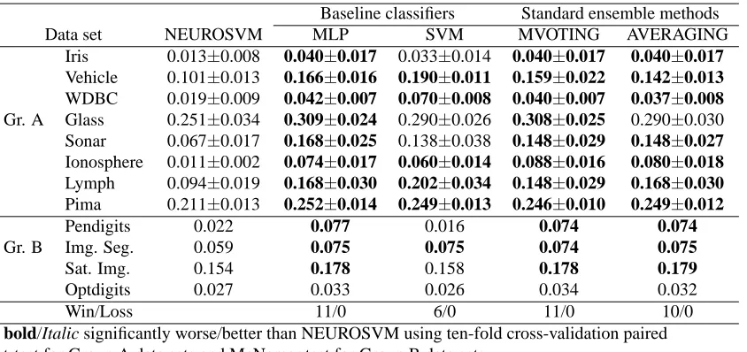
We compare the performance of NEUROSVM with MLP, SVM as well as two existing neural ensemble methods. The majority voting and averaging are simple yet effective ensemble methods. In Table 7, test error results of NEUROSVM, MLP, SVM, majority voting and averaging are shown. In Table 7, majority voting ensemble method is denoted by MVOTING while the average ensemble method is denoted by AVERAGING. The results in Table 7 show that based on the paired t-test for Group A data sets and McNemar test for Group B data sets NEUROSVM is significantly better than the baseline classifiers for 11 data sets when compared with MLP and for 6 data sets when compared with SVM.
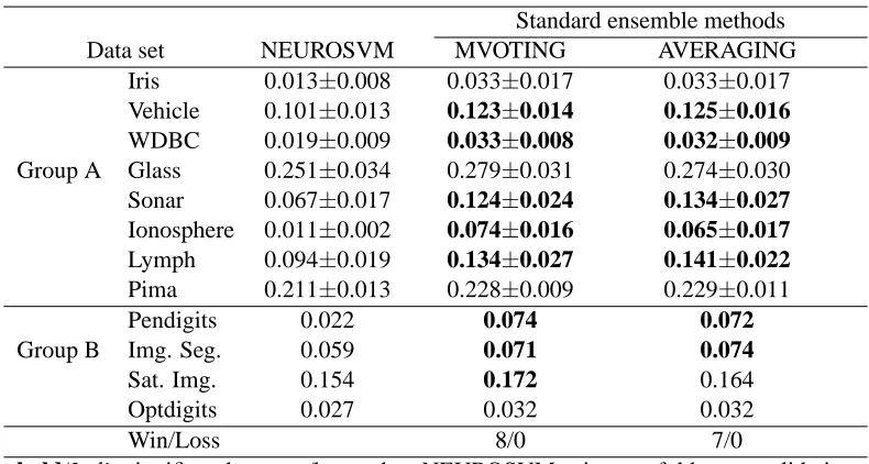
Note that the results of MVOTING and AVERAGING in Table 7 are obtained using the same combinations of networks (SFMs) that are used in the FM of NEUROSVM. From Table 7 we see that NEUROSVM performs significantly better than the standard ensemble methods for 11 data sets when compared with majority voting and for 10 data sets when compared with averaging.
As a summary, NEUROSVM is superior to MLP, SVM as well as two ensemble methods for 6 data sets. These data sets are Vehicle, WDBC, Ionosphere, Lymph, Pima and Img. Seg. For four out of remaining six data sets NEUROSVM performs significantly better than MLP, MVOT-ING and AVERAGMVOT-ING. The performance of NEUROSVM and SVM for these four data sets, Iris, Sonar, Pendigits and Sat. Img, is not significantly different. For the Glass data, the performance of NEUROSVM is significantly better than MLP and MVOTING but is not significantly different from that of SVM and AVERAGING. For the Optdigits data set all algorithms perform equally well. No data set is found where two baseline classifiers (MLP and SVM) or two ensemble methods perform better than NEUROSVM.
Data set Selected combinations and(C,γ)pair of these combinations Iris {2, 5}(0.10, 2.00),{3, 5}(0.10, 2.00),{6, 5}(0.10, 0.10),
{5, 3}(0.10, 2.00),{7, 6}(0.10, 5.00),{5, 6}(0.10, 1.00), {5, 6}(0.001, 0.0001),{5, 6}(0.50, 10.00),
{7, 6}(1000.00, 0.80),{2, 5}(0.10, 2.00)
Vehicle {11, 13}(1.00, 0.20),{9, 7}(1000.00, 2.00),{12, 13}(20.00, 0.80), {10, 5}(0.50, 0.10),{12, 13}(1000.00, 0.40),{12, 14}(1000.00, 2.00), {8, 13}(1000.00, 0.001),{12, 13}(0.20, 1.00),
{11, 6, 10, 13}(1.00, 0.40),{11, 8}(20.00, 0.01)
WDBC {10, 15}(0.50, 0.20),{6, 7}(0.001, 0.0001),{8, 12}(20.00, 0.20), {7, 10}(0.10, 5.00),{8, 10}(0.20, 20.00),{8, 7}(0.50, 0.40), {15, 7}(5.00, 0.40),{7, 8}(0.01, 0.40),{6, 9}(0.01, 0.40), {9, 7}(0.50, 0.01)
Group A Glass {11, 15, 9}(1000.00, 0.01),{7, 8}(1.00, 2.00),{13, 7}(1.00, 5.00), {11, 10}(2.00, 10.00),{9, 6}(1000.00, 0.01),{12, 14, 8}(0.50. 0.20), {5, 4}(5.00, 0.40),{11, 14}(0.10, 0.20),{12, 8, 6}(10.00, 0.10), {14, 15}(1000.00, 0.01)
Sonar {12, 30}(0.20, 2.00),{35, 5}(100.00, 0.10),{30, 7, 10}(0.20, 2.00), {5, 7}(0.50, 5.00),{20, 30}(1.00, 2.00),{7, 9}(2.00, 0.01),
{25, 20}(1.00, 5.00),{7, 10}(0.10, 0.10),{7, 12}(0.10, 0.20), {15, 7}(2.00, 0.01)
Ionosphere {7, 10}(0.001, 0.0001),{7, 8}(0.001, 0.0001),{9, 8}(0.001, 0.0001), {9, 8}(0.001, 0.0001),{8, 9}(0.001, 0.0001),{7, 8}(0.001, 0.0001), {8, 7}(0.001, 0.0001),{8, 10}(0.001, 0.0001),{6, 5}(0.001, 0.0001), {6, 7}(0.001, 0.0001)
Lymph {6, 5}(0.10, 2.00),{6, 7}(20.00, 0.40),{9, 8}(5.00, 0.10), {10, 7}(0.10, 0.20),{9, 12}(0.10, 2.00),{8, 6}(0.10, 0.10), {7, 9}(2.00, 5.00),{7, 8}(0.10, 0.10),{9, 6}(0.50, 0.20), {10, 12, 8, 9}(0.20, 0.01)
Pima {6, 5}(5.00, 100.00),{5, 6}(0.10, 100.00),{6, 7}(5.00, 0.40), {5, 6}(0.50, 1.00),{7, 6}(1000, 0.40),{6, 5}(0.20, 100.00), {5, 6}(1.00, 10000.00),{7, 5}(10.00, 20.00),{5, 7}(20.00, 0.40), {6, 5}(100.00, 0.10)
Pendigits {15, 20, 10}(20.00, 0.10) Group B Img. Seg. {12, 15}(10.00, 1.00)
Sat. Img. {7, 6}(100.00, 0.40) Optdigits {30, 25}(2.00, 0.10)
Table 6: The combination of SFMs and(C,γ) pair for NEUROSVM selected by cross-validation for each of the twelve data sets
Baseline classifiers Standard ensemble methods
Data set NEUROSVM MLP SVM MVOTING AVERAGING
Iris 0.013±0.008 0.040±0.017 0.033±0.014 0.040±0.017 0.040±0.017
Vehicle 0.101±0.013 0.166±0.016 0.190±0.011 0.159±0.022 0.142±0.013
WDBC 0.019±0.009 0.042±0.007 0.070±0.008 0.040±0.007 0.037±0.008
Gr. A Glass 0.251±0.034 0.309±0.024 0.290±0.026 0.308±0.025 0.290±0.030 Sonar 0.067±0.017 0.168±0.025 0.138±0.038 0.148±0.029 0.148±0.027
Ionosphere 0.011±0.002 0.074±0.017 0.060±0.014 0.088±0.016 0.080±0.018
Lymph 0.094±0.019 0.168±0.030 0.202±0.034 0.148±0.029 0.168±0.030
Pima 0.211±0.013 0.252±0.014 0.249±0.013 0.246±0.010 0.249±0.012
Pendigits 0.022 0.077 0.016 0.074 0.074
Gr. B Img. Seg. 0.059 0.075 0.075 0.074 0.075
Sat. Img. 0.154 0.178 0.158 0.178 0.179
Optdigits 0.027 0.033 0.026 0.034 0.032
Win/Loss 11/0 6/0 11/0 10/0
bold/Italic significantly worse/better than NEUROSVM using ten-fold cross-validation paired
t-test for Group A data sets and McNemar test for Group B data sets.
Table 7: Performance comparison of NEUROSVM with baseline classifiers and standard ensemble methods
the standard ensemble methods for 8 data sets when compared with majority voting and for 7 data sets when compared with averaging. Here also no data set is found where two ensemble methods perform better than NEUROSVM. Hence we can conclude that NEUROSVM performs consistently better than majority voting and averaging.
3.3.5 PERFORMANCECOMPARISON OFOTHERVARIANTS OFNEUROSVMWITHBASELINE
CLASSIFIERS ANDSTANDARDENSEMBLEMETHODS
As stated earlier, for the proposed architecture, in the classification module we can use other tools also. Here we demonstrate the effect of using MLP and RBF neural networks in the classification module instead of SVM. We termed these two architectures as NMLP and NRBF respectively. The combination of SFMs and the number of hidden nodes for MLP and RBF networks in the classification module are selected using double ten-fold cross-validation for Group A data sets and using ten-fold cross-validation for Group B data sets. The performance comparison of these variants of NEUROSVM with the original NEUROSVM is shown in Table 10. From Table 10, we see that original NEUROSVM is significantly better than other variants for 4 data sets when compared with NMLP and better than 2 data sets when compared with NRBF. The performance of NEUROSVM and NMLP is equally well for 8 data sets. There is no significant difference in performance between NEUROSVM and NRBF for 10 data sets. For six out of twelve data sets, all three variants of the proposed architecture perform equally well. So, proposed architecture can be considered a general one.
Selected combinations
Data set MVOTING AVERAGING
Iris {2, 5},{3, 5},{6, 5},{6, 3}, {2, 5},{3, 5},{6, 5},{6, 8}, {7, 6},{5, 6},{5, 6},{5, 6}, {7, 6},{5, 6},{5, 6},{5, 6},
{7, 6},{2, 5} {7, 6},{2, 5}
Vehicle {9, 13, 10, 5},{13, 7, 8}, {11, 10},{13, 9},{12, 13, 9}, {10, 13, 9},{13, 12},{13, 7}, {10, 5},{13, 7},{12, 14, 8}, {12, 14, 8},{9, 13, 12},{11, 9}, {9, 8, 13},{13, 11},
{11, 6, 13},{14, 10} {11, 6, 10},{11, 14} WDBC {10, 7},{6, 8, 9},{8, 10}, {10, 9},{6, 7},{15, 12},
{12, 7, 15},{8, 9},{8, 7}, {12, 8},{8, 9},{8, 7}, {15, 7},{8, 10},{6, 9},{9, 7} {15, 7},{7, 8},{6, 9},{9, 7} Group A Glass {15, 4},{12, 13},{12, 7, 14}, {15, 9},{13, 7},{7, 14},
{12, 10},{15, 6},{10, 8},{14, 8}, {15, 10},{10, 6},{12, 9},{4, 8}, {11, 10},{12, 8},{11, 12} {11, 13},{8, 9},{11, 12} Sonar {25, 12},{20, 5},{7, 10},{5, 7}, {25, 12},{20, 5},{7, 10},
{20, 15},{25, 7},{15, 10}, {5, 7},{20, 15},{25, 7},{15, 10}, {7, 10},{7, 12, 15},{15, 7} {7, 10},{7, 12},{10, 7}
Ionosphere {7, 10},{9, 8},{8, 12},{9, 15}, {7, 10},{9, 8},{9, 12},{15, 8}, {8, 10},{7, 8},{8, 7},{8, 20}, {8, 12},{7, 8},{8, 7},{8, 15}, {6, 5},{12, 20} {6, 5},{15, 12}
Lymph {6, 5},{6, 7},{9, 8},{10, 7}, {9, 5},{6, 7},{9, 8},{10, 7}, {9, 12},{8, 6},{10, 8, 9}, {6, 20},{10, 6},{10, 9}, {7, 8},{9, 6},{8, 9} {7, 8},{8, 6},{8, 9}
Pima {8, 9},{9, 8},{6, 7},{6, 8}, {9, 5},{9, 6},{6, 10},{5, 8}, {10, 8},{7, 8},{7, 5},{8, 10}, {6, 8},{5, 8},{6, 8},{8, 9}, {8, 10},{6, 7} {5, 8},{6, 7}
Pendigits {15, 18, 12} {15, 18, 20} Group B Img. Seg. {8, 15} {7, 8, 10, 15}
Sat. Img. {9, 7, 10, 6} {8, 9, 7, 10, 6} Optdigits {35, 40, 20} {35, 40}
Table 8: The combination of SFMs for MVOTING and AVERAGING selected by cross-validation for each of the twelve data sets
used in the FM of NMLP and NRBF respectively. From Table 11 we can see that NMLP performs significantly better than baseline classifiers for 8 data sets when compared with MLP and better than 5 data sets when compared with SVM. The NMLP performs significantly better than MVOTING on 8 data sets. It also performs significantly better than AVERAGING for 7 data sets. From Table 12, it is observed that NRBF performs significantly better than MLP on 8 data sets and it is better than SVM for 4 data sets. The SVM performs significantly better than NRBF only with one data set. When compared with the standard ensemble methods the NRBF is found to perform significantly better for majority of the data sets. For example, NRBF performs significantly better than majority voting for 8 data sets and better than averaging for 7 data sets.
Standard ensemble methods
Data set NEUROSVM MVOTING AVERAGING
Iris 0.013±0.008 0.033±0.017 0.033±0.017
Vehicle 0.101±0.013 0.123±0.014 0.125±0.016
WDBC 0.019±0.009 0.033±0.008 0.032±0.009
Group A Glass 0.251±0.034 0.279±0.031 0.274±0.030
Sonar 0.067±0.017 0.124±0.024 0.134±0.027
Ionosphere 0.011±0.002 0.074±0.016 0.065±0.017
Lymph 0.094±0.019 0.134±0.027 0.141±0.022
Pima 0.211±0.013 0.228±0.009 0.229±0.011
Pendigits 0.022 0.074 0.072
Group B Img. Seg. 0.059 0.071 0.074
Sat. Img. 0.154 0.172 0.164
Optdigits 0.027 0.032 0.032
Win/Loss 8/0 7/0
bold/Italic significantly worse/better than NEUROSVM using ten-fold cross-validation paired t-test for Group A data sets and McNemar test for Group B data sets.
Table 9: Performance comparison of NEUROSVM, MVOTING and AVERAGING for selected combinations with corresponding algorithm
Data set NEUROSVM NMLP NRBF
Iris 0.013±0.008 0.027±0.014 0.013±0.013
Vehicle 0.101±0.013 0.116±0.013 0.114±0.014
WDBC 0.019±0.009 0.030±0.008 0.019±0.009
Group A Glass 0.251±0.034 0.255±0.026 0.253±0.024
Sonar 0.067±0.017 0.119±0.029 0.057±0.015
Ionosphere 0.011±0.002 0.062±0.016 0.045±0.013
Lymph 0.094±0.019 0.135±0.025 0.101±0.020
Pima 0.211±0.013 0.199±0.009 0.194±0.012
Pendigits 0.022 0.023 0.032
Group B Img. Seg. 0.059 0.063 0.067
Sat. Img. 0.154 0.159 0.171
Optdigits 0.027 0.029 0.029
Win/Loss 4/0 2/0
bold/Italic significantly worse/better than NEUROSVM using ten-fold cross-validation paired t-test for Group A data sets and McNemar test for Group B data sets.
Table 10: Performance comparison of three variants of proposed algorithm
Baseline classifiers Standard ensemble methods
Data set NMLP MLP SVM MVOTING AVERAGING
Iris 0.027±0.014 0.040±0.017 0.033±0.014 0.040±0.017 0.040±0.017 Vehicle 0.116±0.013 0.166±0.016 0.190±0.011 0.153±0.013 0.151±0.015
WDBC 0.030±0.008 0.042±0.007 0.070±0.008 0.044±0.008 0.035±0.008 Gr. A Glass 0.255±0.026 0.309±0.024 0.290±0.026 0.294±0.030 0.294±0.030
Sonar 0.119±0.029 0.168±0.025 0.138±0.038 0.144±0.021 0.139±0.027
Ionosphere 0.062±0.016 0.074±0.017 0.060±0.014 0.093±0.019 0.068±0.016 Lymph 0.135±0.025 0.168±0.030 0.202±0.034 0.155±0.026 0.161±0.028 Pima 0.199±0.009 0.252±0.014 0.249±0.013 0.245±0.010 0.238±0.011
Pendigits 0.023 0.077 0.016 0.074 0.072
Gr. B Img. Seg. 0.063 0.075 0.075 0.083 0.078
Sat. Img. 0.159 0.178 0.158 0.176 0.168
Optdigits 0.029 0.033 0.026 0.033 0.036
Win/Loss 8/0 5/0 8/0 7/0
bold/Italic significantly worse/better than NMLP using ten-fold cross-validation paired t-test
for Group A data sets and McNemar test for Group B data sets.
Table 11: Performance comparison of NMLP with baseline classifiers and standard ensemble meth-ods
Baseline classifiers Standard ensemble methods
Data set NRBF MLP SVM MVOTING AVERAGING
Iris 0.013±0.013 0.040±0.017 0.033±0.014 0.040±0.017 0.040±0.017 Vehicle 0.114±0.014 0.166±0.016 0.190±0.011 0.148±0.018 0.137±0.013
WDBC 0.019±0.009 0.042±0.007 0.070±0.008 0.042±0.007 0.040±0.007
Gr. A Glass 0.253±0.024 0.309±0.024 0.290±0.026 0.309±0.029 0.295±0.040 Sonar 0.057±0.015 0.168±0.025 0.138±0.038 0.153±0.027 0.153±0.030
Ionosphere 0.045±0.013 0.074±0.017 0.060±0.014 0.091±0.017 0.077±0.018
Lymph 0.101±0.020 0.168±0.030 0.202±0.034 0.161±0.031 0.189±0.031
Pima 0.194±0.012 0.252±0.014 0.249±0.013 0.252±0.014 0.247±0.011
Pendigits 0.032 0.077 0.016 0.074 0.075
Gr. B Img. Seg. 0.067 0.075 0.075 0.074 0.075
Sat. Img. 0.171 0.178 0.158 0.172 0.167
Optdigits 0.029 0.033 0.026 0.033 0.033
Win/Loss 8/0 4/1 8/0 7/0
bold/Italic significantly worse/better than NRBF using ten-fold cross-validation paired t-test
for Group A data sets and McNemar test for Group B data sets.
Table 12: Performance comparison of NRBF with baseline classifiers and standard ensemble meth-ods
3.4 Controlled Experiments - Avoiding Full Training of Networks for Feature Extraction
We have conducted the experiments as before for NEUROSVM except we stop the training of MLPs to construct SFMs only after 100 iterations. In this case, we have obtained the test error of 0.135±0.087 for Sonar and 0.023 for Optdigits data sets. By statistical test we observe that these errors are not significantly different from the previous NEUROSVM errors when the MLPs were fully trained.
4. The Kernel Independence of NEUROSVM
In this section we shall illustrate an attractive feature of NEUROSVM, its kernel independence. In order to perform such study we choose three kernels for SVM: linear, RBF and polynomial. We choose these kernels also for SVMs in the classification module of NEUROSVM. The different kernels are tried with a set of parameters. We perform ten-fold (double ten-fold for Group A data sets) cross-validation to select the best parameter set for each kernel of SVM. We also conducted cross-validation experiments to select the best combination of SFMs and hyper parameters of NEU-ROSVM for each of three choices of kernel. For the RBF kernel we choose 12 different C and 15 different γresulting 180 pairs. Similarly, for the polynomial kernel we choose 12 different C, 5 different degrees d and 7 different scaling coefficients of dot products s resulting 420 triplets and 12 different C are used in linear kernel. The values of C andγare presented in Section 3.3.2. The five values of d for the polynomial kernel are 2, 3, 4, 5 and 6. The seven different choices of s are 0.001, 0.01, 0.10, 1.00, 10.00, 100.00 and 1000.00.
In Figure 4, the test errors of SVM and NEUROSVM with three choices of kernel for the twelve data sets are shown. It is clear from Figures 4(b)-4(h) that the performance of SVM significantly depends on the choice of kernels for Vehicle, WDBC, Glass, Sonar, Ionosphere, Lymph and Pima data sets respectively. Also the kernel dependency of SVM is noticeable for the data sets Iris, Pendigits, Img. Seg. and Optdigits (Figure 4(a), 4(i), 4(j) and 4(l)). Only for the Sat. Img. the SVM produces almost the same test errors for all three choices of kernel. On the other hand, from Figures 4(a)-4(l) we see that the performance of NEUROSVM for eight (out of the twelve) data sets practically does not depend on the choice of kernels. To observe it more closely for each data set we find out the difference of percentage errors between the maximum and minimum errors produce by the three kernels for SVM and NEUROSVM (Table 13). To explain the entries in Table 13, consider the WDBC data set. The test errors produced by SVM on WDBC data set with the three kernels are 0.049, 0.070 and 0.095 respectively. Hence the minimum and maximum errors are 0.049 and 0.095 respectively. So, the difference in error rates and hence the percentage are 0.046 and 4.60% respectively. Whereas the test error rates for NEUROSVM on WDBC data set with the three kernels are 0.023, 0.019 and 0.023 respectively. Here the minimum, maximum and percentage of difference of these two errors are 0.019, 0.023 and 0.40% respectively. From Table 13, it is clear that for eight data sets the performance of NEUROSVM using the three kernels remains almost the same (with error less than 1%). On the other hand, with SVM only for Sat. Img. the difference is less than 1%. Thus NEUROSVM is found to perform equally well with different choices of kernels of the SVM in the classification module.
5. Conclusions
Differences of the percentage error
Data set SVM NEUROSVM
Iris 1.40% 0.00%
Vehicle 4.10% 0.60%
WDBC 4.60% 0.40%
Glass 10.80% 0.00%
Sonar 8.40% 2.30%
Ionosphere 6.50% 2.10%
Lymph 4.80% 2.00%
Pima 9.30% 1.40%
Pendigits 2.70% 0.10%
Img. Seg. 1.90% 0.90%
Sat. Img. 0.20% 0.20%
Optdigits 1.40% 0.10%
Table 13: Differences of the percentage errors between the maximum and minimum errors pro-duced by linear, RBF and polynomial kernels for SVM and NEUROSVM
the FM, we have used MLP, while for the CM we have used SVM resulting in the classifier, called NEUROSVM. The architecture is general in nature and both for FM and CM other tools can be used. We have experimented using RBF and MLP in the CM. We have tested the performance of the proposed system on twelve benchmark data sets and NEUROSVM is found to perform consistently better than MLP and SVM. The performance of NEUROSVM is also better than the ensemble methods based on majority voting and averaging. A noticeable feature of NEUROSVM is that nonlinear NEUROSVM and linear NEUROSVM perform equally well on all data sets tried.
Other advantages of NEUROSVM are as follows:
• For large data sets, it may not be necessary to make a full training of the MLPs in the FM because in an MLP, the extraction of the salient feature of the data is done at the beginning of the training.
• Typically the number of nodes in the hidden layer of MLPs is much smaller than the number of the input nodes, and one does not need many feature extraction sub-modules. Hence, the dimensionality of the input for the SVMs (or MLP/RBF) in the classification module can be reduced compared to the original dimension of the input. So, for solving bioinformatics problems such as protein secondary structure prediction or protein fold recognition such an architecture may be very useful.
• It may be viewed as an implicit fusion of multiple classifiers and hence the improvement in performance is expected.
more theoretical view of our proposed method that may help further explain the results reported here.
Appendix A. Procedure DataPreparation
Input: A data set X
Output: Training and test data sets Algorithm:
1. if X belongs to Group A then 2. Set no o f f old=10.
3. X is randomly partitioned into 10 subsets Xi; i=1,2, . . . ,10
such that, X= S10
i=1
Xi,Xi∩Xj=φ,i6= j.
4. Get the training set for fold i of X as X Ti= S j6=i
Xj and the test data set is
X Tei=Xi. So we get 10 training-test set(X Ti,X Tei),i=1,2, ,10. 5. else /* for Group B data sets */
6. Set no o f f old=1.
7. Let the training set be X T1and the test set be X Te1. 8. end if
End DataPreparation
NB: For a given data set (in Group A), the Procedure DataPreparation returns the same outer level ten-folds to RunMLP, RunSVM and RunNEUROSVM.
Appendix B. Procedure RunMLP
Input: A data set X.
A set of hidden nodes H={h1,h2, . . . ,hm}. Output: Test error of MLP on X
Algorithm:
1. Perform DataPreparation 2. for i = 1 to no o f f old
/* To choose the optimal network size for X Ti, we use ten-fold cross-validation experiment on X Ti */
3. X Ti is divided into 10 equal (or almost equal) parts Zj; j=1,2, . . . ,10
such that, X Ti= 10
S
j=1
Zj,Zj∩Zk=φ,j6=k .
4. Get the training set for fold j of X Ti as ZTj= S k6=j
Zk and the validation
set as ZVj=Zj. So we get 10 training-validation set(ZTj,ZVj),
j=1,2, . . . ,10 for fold i of X . 5. for each a in{h1,h2, . . . ,hm} 6. for j = 1 to 10
8. end for /* end for j */
9. The average validation error for an architecture a related to X Tiof the
original fold(X Ti,X Tei)is ¯eai =101 10
∑
j=1
eaj.
10. end for /* end of for a */ 11. Let ¯eki =min
a {e¯ a
i}, then we choose k as the optimal architecture for fold X Ti. 12. Train a network (MLP) for architecture k with training data X Tiand find
test error on X Tei. Let the test error with fold(X Ti,X Tei)be Ei. 13. end for /* end of for i */
14. Find average test error ¯E= no o f f old1
no o f f old
∑
i=1
Ei.
End RunMLP
Appendix C. Procedure RunSVM
Input: A data set X .
A set of 12 choices of C and 15 choices ofγfor RBF kernel resulting in a total of 180 pairs of(C,γ).
Output: Test error of SVM on X Algorithm:
1. Perform DataPreparation 2. for i = 1 to no o f f old
/* To choose the best(C,γ)pair for X Ti, we use ten-fold cross-validation experiment on X Ti */
3-4. Same as steps 3-4 of RunMLP 5. for each(Ck,γk)pair on 180 pairs 6. for j = 1 to 10
7. Train SVM with parameters(Ck,γk)of RBF kernel for training data ZTjand find validation error on ZVj.
Let the validation error with fold(ZTj,ZVj)be ekj. 8. end for /* end of for j */
9. The average validation error for(Ck,γk)pair related to X Tiof the
original fold(X Ti,X Tei)is ¯eki = 10
∑
j=1
ekj.
10. end for /* end of for(Ck,γk)*/ 11. Let ¯emi =min
k {e¯ k
i}, then we choose(Cm,γm)pair as the best hyper parameters for fold X Ti.
12. Train SVM with RBF kernel and(Cm,γm)pair with training data X Tiand find test error on X Tei. Let the test error with fold(X Ti,X Tei)be Ei. 13. end for /* end of for i */
14. Find average test error ¯E= no o f f old1 no o f f old∑ i=1
Ei.