Fast and Scalable Local Kernel Machines

Fast and Scalable Local Kernel Machines

Nicola Segata [email protected]

Enrico Blanzieri [email protected]

Department of Information Engineering and Computer Science University of Trento

Trento, Italy

Editor: L´eon Bottou

Abstract

A computationally efficient approach to local learning with kernel methods is presented. The Fast

Local Kernel Support Vector Machine (FaLK-SVM) trains a set of local SVMs on redundant neigh-bourhoods in the training set and an appropriate model for each query point is selected at testing time according to a proximity strategy. Supported by a recent result by Zakai and Ritov (2009) relat-ing consistency and localizability, our approach achieves high classification accuracies by dividrelat-ing the separation function in local optimisation problems that can be handled very efficiently from the computational viewpoint. The introduction of a fast local model selection further speeds-up the learning process. Learning and complexity bounds are derived forFaLK-SVM, and the empirical evaluation of the approach (with data sets up to 3 million points) showed that it is much faster and more accurate and scalable than state-of-the-art accurate and approximated SVM solvers at least for non high-dimensional data sets. More generally, we show that locality can be an important factor to sensibly speed-up learning approaches and kernel methods, differently from other recent techniques that tend to dismiss local information in order to improve scalability.

Keywords: locality, kernel methods, local learning algorithms, support vector machines,

instance-based learning

1. Introduction

Efficiently processing large amount of data is one of the challenges of current research in kernel methods. Although most of the recently proposed techniques are based on different approaches, their common assumption is that scalability can be obtained by limiting or reducing the complex-ity of the decision function. In fact, very fast training algorithms have been developed for linear SVM (Keerthi and DeCoste, 2005; Collins et al., 2008; Chang et al., 2008; Bordes et al., 2009; Fan et al., 2008), and indeed they are effective when the linear separation is a good choice such as in high-dimensionality problems. Other approaches permit the non-linear feature space setting, but they limit the complexity by working with a reduced number of examples or a small set of sup-port vectors (Lee and Mangasarian, 2001), using active and online example selection (Bordes et al., 2005; Bordes and Bottou, 2005) or bounding the number of basis functions (Keerthi et al., 2006; Joachims and Yu, 2009).

is thus to trade locality for scalability permitting, with a potentially high level of under-fitting, to achieve a fast convergence to an approximated solution of the optimisation problem.

We show here that locality is not necessary related to computational inefficiency, but, instead, it can be the key factor to obtain very fast kernel methods without the need to smooth locally the global decision function. In our proposed approach, the model is formed by a set of accurate lo-cal models trained on fixed-cardinality sub-regions of the training set and the prediction module uses for each query point the more appropriate local model. In this setting, we are not approximat-ing with some level of inaccuracy the original SVM optimisation problem, but we are separately considering different parts of the decision function with the potential advantage of better capturing the local separation. So, instead of locally under-fit the decision function by globally smoothing it like approximated SVM solvers do, we search for decision functions that are locally-calculated and they are very similar (or even better) in terms of accuracy to the global decision function in the proximity of each testing point. This approach is theoretically supported also by the recent result obtained by Zakai and Ritov (2009) that showed how, roughly speaking, “consistency implies local behaviour”.

In this work we present Fast Local Kernel Support Vector Machine (FaLK-SVM), that pre-computes a set of local SVMs covering with adjustable redundancy the whole training set and uses for prediction a model which is the nearest (in terms of neighbourhood rank in feature space) to each

testing point.FaLK-SVMis obtained introducing various strategies, detailed below, to speed-up the

Local SVM approach (see Blanzieri and Melgani, 2006 and Section 3.3). Scalability is obtained approximating the Local SVM approach softening the assumption that the query point must be the central example of the neighbourhood on which the local SVM is trained; in this way we use the same local SVM model for more than one testing point and we can also pre-compute the local models during training. The locality of the approach is regulated by the neighbourhood size k and the method uses all the training points. Starting from the theory of local learning algorithms (Bottou

and Vapnik, 1992; Vapnik and Bottou, 1993) we derive generalisation bounds forFaLK-SVM, and

we analyse the computational complexity stating that, under reasonable assumptions, the training of our technique scales as N log N and the testing as log N where N is the training set size. We also introduce a procedure for local model selection in order to speed-up the selection of the parameters and better capturing local properties of the data. The empirical evaluation (with data sets with up

to 3 million examples) shows thatFaLK-SVMoutperforms accurate and approximated SVM solvers

both in term of generalisation accuracy and computational performances.

of this class of problems is the Forest CoverType data set (Blackard and Dean, 1999) which is a large real data set (more than half a million examples) with bounded dimensionality (54 features) that needs as many examples as possible to increase accuracy. We already showed in a very prelim-inary study (Segata and Blanzieri, 2009c) that our approach on this data set is more accurate than SVM and much faster than both accurate and approximated SVM solvers.

The present contribution can be seen from multiple viewpoints. (i) FaLK-SVM modifies the

Local SVM approach (Blanzieri and Melgani, 2006; Zhang et al., 2006) that showed excellent clas-sification performances but had dramatic computational problems, leading to a scalable Local SVM classifier asymptotically much faster than SVM. (ii) The approach is also an enhancement of the local learning algorithms because the learning process is not delayed until the prediction phase (lazy learning) but the construction of the local models occurs during training (eager learning).

(iii) From a practical viewpoint,FaLK-SVMis a novel kernel method which outperforms accurate

and approximated SVM solvers for non high-dimensional data sets. (iv) For complex classification problems that require an high fraction of support vectors (SVs), we exploit locality to avoid the need of bounding the number of total SVs as existing approximated SVM solvers do for computational reasons. (v) More generally, our approach can also be seen as a framework for localising and make scalable any kernel method, classifier and regressor and in general every data analysis that can be

applied on sub-regions of the entire data set. The proposedFaLK-SVMclassifier and related tools are

freely available with source code as part of the Fast Local Kernel Machine Library (Segata, 2009, FaLKM-lib).

In the next Section we analyse the work on local learning algorithms, Local SVM and fast large margin classifiers that are all related with our work. Section 3 formally introduces some

machine learning tools that we need in order to introduceFaLK-SVMin Section 4 and analyse its

learning bounds, complexity bounds, implementation, local model selection procedure and intuitive interpretation. Section 5 details the empirical evaluation with respect to accurate and approximated approaches.

2. Related Work

Locality is often a crucial component of machine learning systems, although we are not aware of approaches exploiting locality for improving the computational performances. We review in this section those areas that are more related with our approach: local learning algorithms, local support vector machines, approximated and scalable SVM solvers.

2.1 Local Learning Algorithms

Local Risk Minimization principle (Vapnik and Bottou, 1993; Vapnik, 2000). Notice that there are various ways of specifying the degree of locality for LLAs as discussed for instance by Atkeson et al. (1997). Examples of LLAs are the well-known k-Nearest Neighbours (kNN) classifier, the Radial Basis Function networks (Broomhead and Lowe, 1988), and the Local SVM classifier (Blanzieri and Melgani, 2006; Zhang et al., 2006) described in Section 2.2.

Despite their theoretical and practical appeal, LLAs seem not to have been studied in depth in the last few years. This is probably due to the fact that LLAs, as formulated by Bottou and Vapnik (1992), fall in the class of lazy learning (or memory-based learning) that have great overhead on the testing phase, as opposed to eager learning in which the function estimation is performed during training increasing the computational performances of the testing phase.

2.2 Local Support Vector Machines

The main idea of Local SVM, described in details in Section 3.3, is to build at prediction time an example-specific maximal marginal hyperplane based on the set of k-neighbours.

Local SVM is a LLA and was independently proposed by Blanzieri and Melgani (2006, 2008) and by Zhang et al. (2006) and applied respectively to remote sensing and visual recognition tasks. Other successful applications of the approach are detailed by Segata and Blanzieri (2009a) for gen-eral real data sets, by Blanzieri and Bryl (2007) for spam filtering and by Segata, Blanzieri, Delany, and Cunningham (2009b) for noise reduction. Similar approaches have been presented by Yang and Kecman (2008) and applied in the medical domain (Yang and Kecman, 2009) and for face recognition problems (Yang and Kecman, 2010).

However, Local SVM suffers from the high computational cost of the testing phase that com-prises, for each example, (i) the selection of the k nearest neighbours and (ii) the computation of the maximal separating hyperplane on the k examples. An attempt to computationally improve the Local SVM approach of Zhang et al. (2006) has been proposed by Cheng et al. (2007) where the idea is to train multiple SVMs on clusters found by a variant of k-means, called MagKmeans, that introduces in the clustering criterion the requirement that the clusters cannot have unbalanced class cardinalities. However the method does not follow directly the idea of Local SVM, the main difference being that it can build only local linear models and the size of the clusters is not fixed (MagKmeans does not have constraints on the cardinalities and the balancing requirement can cause the detection of clusters with high cardinalities). The achieved computational performances are bet-ter than their formulation of Local SVM, but worse than global SVM.

2.3 Fast Large Margin Classifiers

The need for fast and scalable kernel-based classifiers led to the development of several methods in the last few years, although considerable attention seems to have been focused especially on linear SVM classifiers. Below, we initially consider the works applicable also to non-linear kernels, successively we review the works on the linear case.

One of the first large-scale maximal margin learning that can use non-linear kernel functions is

represented by Core Vector Machines (Tsang et al., 2005,CVM); reformulating the SVM approach

Ball Vector Machines (Tsang et al., 2007,BVM) are a modification ofCVMin which the minimality of the enclosing balls is not required, because the radius of the ball is fixed. The resulting clas-sifier improves the computational performances. Another approach based on an online setting of

the SVM optimisation problem has been proposed by Bordes et al. (2005,LASVM) and by Bordes

and Bottou (2005) and it is an algorithm that converges to the SVM solution. It has been shown that competitive accuracies can be achieved also after a single pass over the training set. The ap-proach can be seen as a SVM solver that includes a support vector removal step. In addition, several strategies for active training-points selection can further improve computational and generalisation

performances. Formulating the optimisation problem in the primal, Keerthi et al. (2006, SpSVM)

proposed a method that bounds the number of basis functions considered and thus the computa-tional complexity. Increasing the cardinality of the basis function set allows the method to converge to the SVM solution. A greedy strategy guides the choice of the basis functions to be included in

the working set. Collobert et al. (2006,USVM) showed that softening the convex setting of maximal

margin classifiers using a non-convex loss function can bring computational advantage over the cor-responding standard convex problem. The non-convex problem is solved using the concave-convex

procedure (Yuille and Rangarajan, 2003). Recently, the Cutting-Plane Subspace Pursuit (Joachims

and Yu, 2009,CPSP) based on cutting-plane training (Joachims et al., 2009) has been proposed; it

permits to learn maximal-margin decision functions in the feature space using arbitrary basis vectors instead of the support vectors only. This can results in sparser solutions increasing the testing and training computational performances especially for high-dimensional data sets. Although not

al-ways considered a method for large-scale learning,LibSVM(Chang and Lin, 2001) demonstrated to

be competitive with approximated approaches from the computational viewpoint.LibSVMis a SVM

solver implementing a SMO-type decomposition method proposed by Fan et al. (2005) integrating it with caching and shrinking (Joachims, 1999).

Large margin classifiers can also achieve scalability using subsampling-based approaches that train the model on a relatively small subset of the whole training set. However, the accuracy of SVM with subsampling can decrease due to the loss of information contained in the discarded training points. The decreasing of accuracy with respect to SVM without subsampling is more dramatic when a complex decision function is needed. In these cases the accuracy problems can be mitigated or reduced by developing an ensemble of classifiers. Bootstrap aggregating (bagging) by Breiman (1996) is an effective strategy to perform accurate classification using an ensemble of classifiers trained on subsets of the training set (using uniform sampling with replacement) that can also overcome the accuracies of SVM. Bagging with SVM can thus be used for obtaining scalability as long as the advantage of training smaller SVM models on subsets of the training set (that can scale cubically) overcome the disadvantage of training multiple SVMs.

used for non-linear SVM the performances are analysed for the linear case only. LIBLINEAR (Fan et al., 2008) is a fast software package implementing some of the cited works. The common idea of all the proposed methods is that the advantage of having a method that uses a huge number of training points overcomes the disadvantage of approximating the decision function with a linear model. This is effective, as explicitly noticed in almost all the cited works, when the dimensionality is very large and thus the problem is very sparse. This is, for example, the typical situation of text document classification. However, when the needed decision function is highly non-linear and the intrinsic dimensionality of the space is relatively small, the linear SVM approach cannot compete with SVM using non-linear kernels in terms of generalisation accuracy. Apart from the generalisa-tion ability also the computageneralisa-tional performances can be compromised in these cases, because the algorithm cannot find a good decision function and so convergence problems can occur.

3. Preliminaries

In order to introduce our approach, we need to analyse the formulation of kNN, SVM, kNNSVM and cover trees.

Here and in the following of the paper, we consider a binary class classification with examples

(xi,yi)∈

H

X

H

inner producth·,·iand normk · k. Extensions to multi-class problems will be explicitly discussed.

3.1 The k Nearest Neighbour Algorithm

Given an example x′∈

H

X

corresponds to define a function rx′ :{1, . . . ,N} → {1, . . . ,N}that recursively reorders the indexes

of the N points in

X

  

 

rx′(1) =argmin

i=1,...,N

kxi−x′k

rx′(j) =argmin

i=1,...,N

kxi−x′k i6=rx′(1), . . . ,r_x′(j−1) for j=2, . . . ,N.

In this way, xrx′(j)is the example in the j-th position in terms of distance from x

′_{, namely the}

j-th nearest neighbour,kxr_x′(j)−x

′_{kis its distance from x}′_{and y}

r_x′(j)is its class. In other terms:

j<k⇒ kx_r x′(j)−x

′_{k ≤ kx}

rx′(k)−x ′_k.

Given the above definition, the majority decision rule of kNN for binary classification problems is defined by

kNN(x) =sign

k

∑

yrx(i) !

.

3.2 Support Vector Machines

SVMs (Cortes and Vapnik, 1995) are classifiers with sound foundations in statistical learning the-ory (Vapnik, 2000). The decision rule is

SVM(x) =sign(hw,Φ(x)iF+b)

where Φ(x):

H

F

F

producth·,·iF. The parameters w∈

F

the expected risk while minimising the empirical risk. The minimisation of the complexity term is

achieved by the minimisation of the quantity1₂· kwk2_{, which is equivalent to the maximisation of the}

margin between the classes. In the optimisation problem, the violation of the margin is prevented by the following set of constraints:

yi(hw,Φ(xi)iF +b)≥1. (1)

If a linear separation cannot be found in the input or feature space, the soft-margin variant of SVM permits the violation of the margin and the presence of misclassified training examples. This

is possible introducing slack variablesξi(the empirical risk):

yi(hw,Φ(xi)iF+b)≥1−ξi ξi≥0, i=1, . . . ,N. (2)

For soft-margin SVM the optimisation problem with linear penalisation ofξi (L1-norm), becomes

the minimisation of 1₂· kwk2_+C∑

iξi subject to (2). Reformulating such an optimisation problem

with Lagrange multipliersαi(i=1, . . . , N), and introducing a positive definite kernel (PD) function1

K(·,·)that substitutes the scalar product in the feature spacehΦ(xi),Φ(x)iF the decision rule can

be expressed as:

SVM(x) =sign

N

∑

αiyiK(xi,x) +b

! .

Throughout this work, SVM denotes the soft-margin SVM.

The kernel trick avoids the explicit definition of the feature space

F

Φ (Sch¨olkopf and Smola, 2002). Popular kernels are the linear kernel, the radial basis function

kernel, and the homogeneous and inhomogeneous polynomial kernels. Their definitions are:

Klin(x,x′) = hx,x′i Krb f(x,x′) = exp

−kx−_σx′k2,

Khpol(x,x′) = hx,x′id _Kipol_(x,x′_{) = (hx,x}′_i+1)d_.

The maximal separating hyperplane defined by SVM has been shown to have important gener-alisation properties and nice bounds on the VC dimension (Vapnik, 2000).

Multiple methods has been proposed in order to apply the maximal margin principle of SVM on multiple class problems. The more popular are the one-against-all method (Bottou et al., 1994)

which builds a number of binary decision functions equal to the number of classes Ncl, the

one-against-one method (Knerr et al., 1990; Kressel, 1999) which builds Ncl·(Ncl−1)/2 binary decision

functions using voting in the prediction phase, and the Directed Acyclic Graph SVM (Platt et al.,

2000, DAGSVM) which is a modification of the one-against-all method. Other general strategies for reducing the multi-class classification setting to a binary classification problem have been analysed and developed by Allwein et al. (2000). The study carried on by Hsu and Lin (2002) shows that, for SVM, the more effective strategies are the one-against-one and DAGSVM approaches.

3.3 Local SVM: The kNNSVM Classifier

We already introduced the idea of Local SVM in Section 2.2, here we detail kNNSVM which is the formulation of Local SVM proposed by Blanzieri and Melgani (2006, 2008). kNNSVM can be seen as a modification of the SVM approach in order to obtain a LLA able to locally adjust the capacity of the training systems.

In order to classify a given example x′∈

H

transformed feature space

F

this k-neighbourhood. In practice, this means that an SVM is built over the neighbourhood in

F

each test example x′. Accordingly, the constraints in (1) become:

yr_x′(i) w·Φ(xrx′(i)) +b

≥1−ξr_x′(i),with i=1, . . . ,k

where rx′:{1, . . . ,N} → {1, . . . ,N}is a function that reorders the indexes of the training examples

defined as:

  

 

rx′(1) =argmin

i=1,...,N

kΦ(xi)−Φ(x′)k2F

rx′(j) =argmin

i=1,...,N

kΦ(xi)−Φ(x′)k2F i6=rx′(1), . . . ,r_x′(j−1) for j=2, . . . ,N.

(3)

In this way, xr_x′(j) is the example in the j-th position in terms of distance from x′ and thus

j<k⇒ kΦ(xr_x′(j))−Φ(x′)kF ≤ kΦ(xrx′(k))−Φ(x ′_)k

F because of the monotonicity of the quadratic

operator. The computation is expressed in terms of kernels as:

||Φ(x)−Φ(x′)||2F = hΦ(x),Φ(x)iF +hΦ(x′),Φ(x′)iF−2· hΦ(x),Φ(x′)iF =

= K(x,x) +K(x′,x′)−2·K(x,x′).

If the kernel is the RBF kernel or any polynomial kernels with degree 1, the ordering function is equivalent to the one defined by the Euclidean metric. In general, for some non-linear kernels (other than the RBF kernel) the ordering function can be quite different to that produced using the Euclidean metric.

The decision rule associated with the method for an example x is:

kNNSVM(x) =sign k

∑

αrx(i)yrx(i)K(xrx(i),x) +b !

.

For k=N, the kNNSVM method is the usual SVM whereas, for k=2, the method implemented

built in the feature space, the method has been shown to have a potentially favourable bound on the expectation of the probability of test error with respect to SVM (Blanzieri and Melgani, 2008).

The generalisation of kNNSVM for multi-class classification can occur locally, that is solving the local multi-class SVM problem, or globally, that is applying the binary kNNSVM classifier on multiple global binary problems. In Segata and Blanzieri (2009a) the adopted strategy for multi-class multi-classification with kNNSVM is the one-against-one strategy applied on the local problems. The choice of the one-against-one approach gave good results in comparison with the same strategy on SVM, but no specific empirical studies have been performed yet to identify the most appropriate strategy for multi-class classification with Local SVM.

3.4 Cover Trees

A cover tree is a data structure introduced by Beygelzimer et al. (2006) for performing exact nearest-neighbour operations in a fast and efficient way. Cover trees can be applied in general metric spaces without any other assumption on their structure and thus also in Hilbert spaces calculating the distances by means of kernel functions using the kernel trick.

In more detail, a cover tree can be viewed as a sub-graph of a navigating net (Krauthgamer and Lee, 2004) and it is a levelled tree in which each level (indexed by a decreasing integer i) is a cover (i.e., is representative) for the level beneath it. Every node of a cover tree T is associated with a point

of a data set S. Denoting with Cithe set of points associated with nodes in T at level i, with b>1 a

constant, and with dist(·,·)the distance function defining the metric of the space, the invariants of

a cover tree are:

Nesting Ci⊂Ci−1

Covering tree For every p∈Ci−1 there exists a q∈Ci such that dist(p,q)<bi and the node in

level i associated with q is a parent of the node in level i−1 associated with p.

Separation For all distinct p,q∈Ci, dist(p,q)>bi.

Intuitively, the nesting invariant means that once a point appears in a level, it is present for every lower level. The covering tree invariant implies that every node has a parent in a higher level such

that the distance between the respective points is less than bi, while separation invariant assures that

the distance between every pair of points associated to the nodes of a level i is higher than bi. In

addition, the root of the tree (called C∞ and containing only one example) is a randomly chosen

example.

Cover trees have state-of-the-art performance for exact nearest neighbour operations for general metrics in low-dimensional spaces both in terms of computational complexity and space require-ments. As theoretically proved by Beygelzimer et al. (2006), the space required by the cover tree

data-structure is linear in the data set size (

O(n)

deletions and exact nearest neighbour queries is logarithmic (

O(

built in

O(n log n)

4. FaLK-SVM: A Fast and Scalable Local Kernel Machine

(Section 4.2). We then describe the prediction mechanism in Section 4.2.2 and our approach for fast local model selection in Section 4.3. Successively, we derive learning bounds for the approach in Section 4.4 before discussing the computational complexity in Section 4.5 and some details about the implementation (Section 4.6).

4.1 Pre-computing the Local Models during Training Phase

For the local approach we are proposing here, we need to generalise the decision rule of kNNSVM to the case in which the local model is trained on the k-neighbourhood of a point distinct, in the

general case, from the query point. A modified decision function for a query point q∈

H

another (possibly different) point t∈

H

kNNSVMt(q) =sign

k

∑

αrt(i)yrt(i)K(xrt(i),q) +b !

(4)

where rt(i)is the kNNSVM ordering function (see above Section 3.3) andαrt(i)and b come from

the training of an SVM on the k-neighbourhood of t in the feature space. In the following we will

refer to kNNSVMt(q)as being centred on t, to t as the centre of the model, and, if t∈

X

the Voronoi cell induced by t in

X

Vt={p∈

H

X

The original decision function of kNNSVM corresponds to the case in which t=q, and thus

kNNSVMq(q) =kNNSVM(q).

kNNSVM requires that the training of an SVM on the k-neighbourhood of the query point must

be performed in the prediction step. This approach is computationally feasible only for problems with few points to test which is a condition that rarely holds in real-world classification problems. In general, we need to speed-up the prediction phase. The first modification of kNNSVM consists in predicting the label of a test point q using the local SVM model built on the k-neighbourhood of

its nearest neighbour in

X

kNNSVMt(q)with t=xrq(1). (5)

Notice that in situations where the k-neighbourhood contains only one class the local model does not find any separation and so it can adopt the majority rule for improving the computational per-formances.

With this formulation the local learning can switch from the lazy learning (Aha, 1997) setting of the original formulation of kNNSVM to the eager learning setting with clear advantages in terms of

prediction step complexity. This is possible computing a local SVM model for each x∈

X

training phase obtaining the sets{(t,kNNSVMt)

t∈

X

model such that t=xrq(1)for each query point q during the testing phase.

This approximation slightly modifies the approach of kNNSVM as a local learning algorithm. Instead of estimating the decision function for a given test example q and thus for a specific point

in the input metric space, we estimate a decision function for each Voronoi cell Vx induced by the

training set in the input metric space. In this way, the construction of the models in the training phase requires the estimation of N local decision functions. The prediction of a test point q is done

using the model built for the Voronoi region in which q lies (Vhwith h=xrq(1)) that can be retrieved

4.2 Reducing the Number of Local Models that Need to Be Trained

The pre-computation of the local models during the training phase introduced above, increases the computational efficiency of the prediction step. However, a considerable overhead is added to the training phase. In fact, the training of an SVM for each training point can be slower than the training of a unique global SVM (especially for non small k values), so we introduce another modification of the method which aims to dramatically reduce the number of SVMs that need to be pre-computed.

The idea is that we can relax the constraint that a query point x′is always evaluated using the model

trained around its nearest training point. The decision function of this approach is

FastLSVM(x) =kNNSVMf(x)(x) (6)

where f :

H

C

X

f(x)which is, accordingly to Equation 4, the centre of the local model that is used to evaluate x.

The set

C

C

Notice that if f(·) =_xr

·(1), we have that

C

X

kNNSVM formulation of Equation 5, and this can happen if we use all the examples in the training

set as centres for local SVM models. In the general case, however, we select only a proper subset

C

X

x(1)∈

C

can be defined as f(x) =xrx(1), but if xr_x(1)∈/

C

principle of locality is preserved and the retrieval of the model is fast at prediction time.

Two aspects need to be addressed now: the strategy to select the subset

C

X

formu-lation of the function f associating each query example with an example in

C

4.2.1 SELECTING THECENTRES OF THELOCALMODELS

The approach we developed for selecting the set

C

the idea that each training point must be in the k′-neighbourhood of at least one centre with k′

being a fixed parameter and k′≤k. From a slightly different viewpoint, we need to cover the entire

training set with a set of hyper-spheres whose centres will be the examples in

C

hyper-sphere contains exactly k′points. We can formalise this idea with the concept of k′-neighbourhood

covering set:

Definition 1 Given k′∈N_{, a k}′_{-neighbourhood covering set of centres}

C

X

[

c∈C

x_rc(i)|i=1, . . . ,k′ =

X

Definition 1 means that the union of the sets of the k′-nearest neighbours of

C

whole training set. Theoretically, for a fixed k′, the minimisation of the number of local SVMs

that we need to train can be obtained computing the SVMs centred on the points contained in the

minimal k′-neighbourhood covering set of centres.

This problem is related to the Set Cover Problem (SC) (Garey and Johnson, 1979; Kearns and Vazirani, 1994; Marchand and Shawe-Taylor, 2003) and to the Minimum Sphere Set Covering

Prob-lem (MSSC) (Chen, 2005). However, in the SC and MSSC probProb-lems one specifies the radius of the

spheres rather than their cardinality in terms of points they contain and it is not required that the centres of the hyperspheres correspond to points in the set. It is easy to show that MSSC is NP-hard but some efficient approximated results are available based on greedy approaches (Chvatal, 1979; Wang et al., 2006), integer and linear programming (Wei and Li, 2008).

In our case, however, we do not need the minimality of the constraints of the k′-neighbourhood

covering set of centres to be strictly satisfied, because training some more local SVMs is acceptable instead of solving an NP-hard problem.

The heuristic procedure we developed can be seen as a modification of the greedy approach for

the MSSC problem (Chvatal, 1979; Wang et al., 2006). The first k′-neighbourhood is selected

ran-domly choosing its centre in

X

that are still not members of other k′-neighbourhoods and are as far as possible from the already

selected centres. The selection of the farthest example, still not included in the k′-neighbourhoods,

as the centre of the next k′-neighbourhood, is the counterpart of the selection of the set of points

having the minimum overlapping with the already covered set of points used by the greedy approach to the MSSC and SC problems.

For detailing the greedy approach we adopt, we need the concepts of minimum and maximum distance between the elements of a set of points A defined respectively as:

d(A) =minkx−x′kwith x,x′∈A and x6=x′

and

D(A) =maxkx−x′kwith x,x′∈A.

In particular, the minimum distance between points in

X

D(X). Our intention is to identify a system of subsets Si⊆

X

d(Si); we can in this way define an ordering on the sets . . .⊂Si+1⊂Si ⊂Si−1⊂. . . such that

. . . >d(Si+1)>d(Si)>d(Si−1)> . . .. With this strategy we can choose the centres of the local

models first in the set Si+1, then in the set Si and so on, thus selecting first the centres that are

assured to be distant at least d(Si+1), then at least d(Si)<d(Si+1)and so on. More in detail, we

require that in the ith set Si⊆

X

are subject to the constraint d(Si)>biwith b>1. The bound on the minimum distance d(Si)thus

varies as powers of b depending on the set Si.

Let us define precisely the system of sets{Si}. The maximum i index of Siis named top and the

minimum is named bot, and they are univocally defined as those indexes satisfying btop−1≤M<

btopand bbot<m≤bbot+1. The Siare recursively defined as:

 



Stop = {choose(X)}

Si = Si+1∪argmax

S∈X\Si+1

(|S|s.t. d(Si+1∪S)>bi) for i=top−1, . . . ,bot , (7)

where choose(A)is a function that selects only one element of the non-empty set A. An example

of choose()for our case can be the following definition that selects the example with the minimum

index:

Notice that, since Sicontains Si+1we have that

Stop={choose(X)} ⊆Stop−1⊆. . .⊆Sbot+1⊆Sbot=

X

and, forcing for definition that d(A) =∞if|A|=1,

d(Stop) =∞>d(Stop−1) =M>d(Stop−2)> . . . >d(Sbot+1)>d(Sbot) =m.

We can now formalise the selection of the centres from

X

is simply the (only) example in Stop. The next centre c2 is chosen among the non-empty Sl sets

obtained removing from Si the first centre c1 and the points in its k′-neighbourhood; in particular

c2 is chosen from the non-empty Sl with highest l. The general case for the cj centre is similar,

with the only difference being that we remove from the Sisets all the centres ct with t<j and their

k′-neighbourhood. More formally:

(

c1 = choose(Stop)

cj = choose(Sl)with l=max(m∈N|Sm\

X

, (9)

where

X

j [

l=1 n

xrcl(h)

h=1, . . . ,k′ o

.

is the union of all the k′-neighbourhoods of the centres already included in

C

We can briefly show that the

C

centres. In fact, the iterative procedure for selecting the centres in

C

function cannot select a point from Sl because all Sj with j=bot, . . . ,top are empty. Since for the

set Sbot we always have that Sbot=

X

X

X

X

situation is equivalent to the constraint of Definition 1, we can conclude that

C

covering set of centres.

Computationally, the selection of the centres from the Sj sets with Equation 9 can be performed

efficiently once the Sj are identified. More problematic is the construction of the nested set of Sj

sets. We can however notice that the Sjsets share some characteristics with the levels of cover trees.

First, from Equation 7 we can easily see that for each Sj set with j<top all the points in it are at

least distant as bj because d(Sj)>bj; this is equivalent to the separation invariant of cover trees

reported in Section 3.4. Second, always from Equation 7 we can conclude that each Sjis contained

in every St set with t<j as also explicated in Equation 8; this is equivalent to the nesting invariant

of cover trees. The only constraint of our strategy to identify the Sj sets that is not respected by

cover trees is the maximality of the set added to each Sjset to obtain Sj+1. However, the procedure

to insert a new point in a cover tree is based on adding it to the highest possible level, and this is an efficient approximation of the maximality constraint we have in Equation 7. Taking all these facts

into consideration, we chose to use the levels of cover tree as the Sj sets from which we select the

centres as reported in Equation 9.

Consequently with the goal of reducing the number of local models, this approach no longer

requires that a local SVM is trained for each training example, but we need to train only|

C

centred on each c∈

C

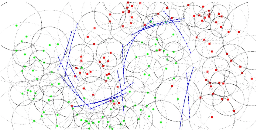
Figure 1: Graphical representation of the proposed approach using local models with k′ = 4,

k=15, and local SVM with RBF kernel. The bold dotted circles highlights the k′

-neighbourhoods covering all the training set (with some unavoidable redundancy), the thin dotted circles denotes the k-neighbourhoods on which the local models are trained. Some k-neighbourhoods do not produce an explicit decision function because entirely composed by points of the same class. The local SVM (with RBF kernel) decision

func-tions are drawn in blue. Notice that, due both to the adoption of the k′-neighbourhood

cover set and to the fact that only a fraction of the neighbourhoods need to be trained, we have only 17 local decision functions for 185 points.

Moreover if a neighbourhood contains only points belonging to one class the local model is the majority rule (specifically, unanimity) and the training of the SVM is avoided.

Figure 1 graphically shows the result of adopting the approach described above on a simple

artificial data set with k and k′ chosen for illustrative purposes. In fact, the example just aims to

show the intuition behind the approach that is instead developed for large data sets and for non-extreme values of the neighbourhood parameters.

From Figure 1 we can also notice that the level of overlapping between k′-neighbourhoods

and thus between k-neighbourhoods depends on the value of k′. If k′ is low, a large number of

k′-neighbourhoods are required to cover the entire training set, whereas if k′ is large fewer k′

-neighbourhoods are needed. The k′parameter thus tune the level of redundancy of the local models.

4.2.2 SELECTING THELOCALMODELS FORTESTINGPOINTS

Once the set of centres

C

select the proper model to use for predicting the label of a test point. A simple strategy we can

testing example. Using the general definition ofFastLSVMof Equation 6 with f(x) =r_xC(1)where

rC corresponds to the reordering function defined in Equation 3 performed on the

C

X

FaLK-SVMc(x) =kNNSVMc(x)where c=xrC

x(1). (10)

FaLK-SVMcis satisfactory from the computational viewpoint, for it performs the nearest neighbour

search on

C

centred on the point for which the testing point itself is the nearest in terms of neighbour ranking.

For example, a testing point q can be closer to c1 than c2 using the Euclidean distance, but at the

same time we can have that q is the i-th nearest neighbour of c1in

X

of c2 with i> j. This is a problem because using the model centred on c2 is better in terms of

proximity. In order to overcome this issue ofFaLK-SVMcwe propose to use, for a testing point q,

the model centred on the training point which is the nearest in terms of the neighbourhood ranking

to its training nearest neighbour. We can do this defining a function cnt :

X

C

way:

cnt(xi) =choose(

n

cz∈

C

)

where h=mint∈ {1, . . . ,k′}

xr_{c j}(t)=xiand cj∈

C

. (11)

The cnt function finds, for each example x, the minimum value h such that x is in the h-neighbourhood

of at least one centre c∈

C

the centre with the minimum index. The existence of h is guaranteed by the k′-neighbourhood

covering strategy. In this way each training point is univocally assigned to a centre and so the

de-cision function of this approximation of Local SVM derivable fromFastLSVMof Equation 6 with

f(x) =cnt(x), and calledFaLK-SVM, is simply:

FaLK-SVM(x) =kNNSVM_cnt(t)(x)where t=x_rx(1). (12)

The association between training points and centres defined by Equation 11 can be efficiently precomputed during the training phase, delaying to the testing phase only the retrieval of the nearest neighbour of the testing point and the evaluation of the local SVM model.

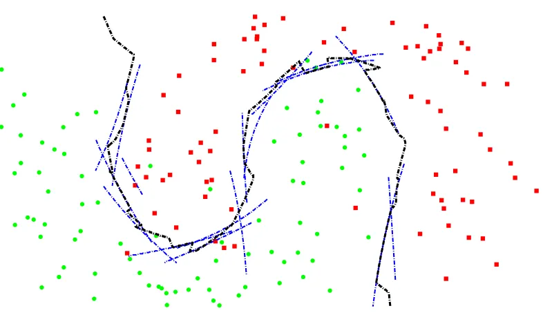
Figure 2 graphically shows the application of theFaLK-SVM(x)prediction strategy on a toy data

set; the training phase for the same data set is illustrated in Figure 1.

FaLK-SVM can be generalised for multi-class problems in the same way of kNNSVM, but in

this paper we focus on binary problems in order to better evaluate the approach.

4.3 FaLK-SVMwith Internal Model Selection:FaLK-SVMl

For training a kernel machine, once a proper kernel is chosen, it is crucial to carefully tune the kernel parameters and, for SVM, to set the soft margin regularisation constant C. Model selection is very often performed estimating the empirical error with different parameter values and a popular

method is theκ-fold cross-validation2with a grid search on parameter space. Given the following

loss function for the two-class classification case

L(y,SVM(x)) =

0 if y=SVM(x)

1, if y6=SVM(x) ,

2. Althoughκ can be confused with the neighbourhood size k or with the kernel function K,κis always used for

Figure 2: Graphical representation of the global decision function (black dotted line) obtained with the local decision functions (the same of Figure 1) using the described approach that uses for each query point the local decision function of the Voronoi region in which it lies.

and partitioning the training set

X

κ-fold cross validation (CV) procedure consists in searching for the parameters that minimise the

average of the losses on

X

X

X

terms of testing accuracies ofκ-fold CV is high, but it adds a computational overhead to the training

phase. In fact, the computational complexity of aκ-fold CV run on a single parameter choice is in

the order ofκtimes the training time; if we have p parameters to set and c possible choices for each

parameter, theκ-fold cross-validation with grid selection isκ·cptimes slower than a single training

of the classifier.

The model selection for FaLK-SVM andFaLK-SVMc can be performed usingκ-fold CV. The

only difference with SVM is that our local kernel machines need to estimate an additional parameter which is the neighbourhood size k (which is however usually chosen in a small set of possible values). However, with the local setting of the classification problem we are discussing in this paper, it is also possible to efficiently tackle the complexity of the model selection phase. Basically, since FaLK-SVMtrains a set of local models, we can perform the model selection in a grid-search setting on a subset of the neighbourhoods. In this way we can efficiently estimate the global parameters of FaLK-SVM without considering all the training points during model selection. The classifier

implementing this approach to model selection is calledFaLK-SVMl.

As a first step for defining the model selection approach of FaLK-SVMl, we define a different

setting of model selection for kNNSVM.

Definition 3 (Localisedκ-fold CV model selection for kNNSVM) The procedure applies the κ -fold CV model selection on the k-neighbourhood of the query point.

However, since the local model is used by kNNSVM only for the central point, the model selec-tion should be performed in order to make the local models predictive especially for the very internal

points. The idea thus consists in selecting theκvalidation sets exclusively from the k′ most

inter-nal points, taking as each corresponding training fold the union of the remaining k′-neighbourhood

points and of the k−k′most external points of the k-neighbourhood.

Definition 4 (k′-internalκ-fold CV model selection for kNNSVM)

The procedure applies the localisedκ-fold CV model selection on the k′-neighbourhood of the query point in the training set adding to each training fold the points in the k-neighbourhood that are not in the k′-neighbourhood with k>k′.

For FaLK-SVM we can apply the k′-internal κ-fold CV for kNNSVM model selection on a

randomly chosen training example and use the resulting parameters for all the local models. In order to be robust the procedure is repeated on more than one k-neighbourhood choosing the parameters

that minimise the average k′-internalκ-fold CV error among the k-neighbourhoods.

Definition 5 (k′-internalκ-fold CV model selection forFaLK-SVM)

The procedure applies the k′-internalκ-fold CV for kNNSVM model selection on the k-neighbour-hoods of 1≤m≤ |

C

The variant of FaLK-SVM that adopts the k′-internal κ-fold CV described in Definition 5 is

namedFaLK-SVMl. SinceFaLK-SVMlselects the local model parameters using a small subset of the

training set, the variance of the error may be higher than the standard cross-validation strategies. However, for huge data sets the standard model selection can be too slow to be applied and, in any case, one may use large values of m to decrease the risk of selecting non-optimal parameters.

4.3.1 A SPECIFICSTRATEGY FORSETTING THERBF KERNELWIDTH

As already proposed by Tsang et al. (2005) and by Segata and Blanzieri (2009b), good choices for

the RBF kernel widthσof SVM are based on the median (or other percentiles) of the distribution of

distances. InFaLK-SVMlwe can thus efficiently estimateσfor each local model simply calculating

the median of the distances in the neighbourhood. This approach has some analogies with standard SVM using a variable RBF kernel width that have good potentialities for classification (Chang et al., 2005). Since other percentiles different from the median can give better accuracy performances, in FaLK-SVMlthe percentile can be a value to set using the k′-internalκ-fold CV approach.

4.4 Generalisation Bounds for kNNSVM andFaLK-SVM

The class of LLAs introduced by Bottou and Vapnik (1992) includes kNNSVM, and can be theo-retically analysed using the framework based on the local risk minimisation (Vapnik and Bottou,

1993; Vapnik, 2000). On the other hand,FaLK-SVMis not a LLA as intended by Bottou and Vapnik

(1992). In fact, LLAs compute the local function for each specific testing point thus delaying the neighbourhood retrieval and model training until the testing point is available. However, we show

We need to recall the bound for the local risk minimisation, which is a generalisation of the global risk minimisation theory.

Theorem 6 (Vapnik (2000)) For a testing point x′ and with probability 1−ηsimultaneously for all bounded functions A≤L(y,f(x,α))≤B,α∈Λ(whereΛis a set of parameters), and all locality functions 0≤T(x,x0,β)≤1,β∈(0,∞), the following inequality holds true:

RLLA(α,β,x′)≤ 1

N∑

N

i=1L(yi,f(xi,α))T(xi,x′,β) + (B−A)γ(N,hΣ)

|_N1∑N_i=1T(xi,x′,β)−γ(N,hβ)|

,

where

γ(N,h) =

r

h ln(2N/h+1)−lnη/2

N ,

and hΣis the VC dimension of the set of functions L(yi,f(xi,α))T(xi,x′,β),α∈Λ,β∈(0,∞)and

hβis the VC dimension of T(xi,x′,β)

For kNNSVM, the loss function is simply

L(yi,f(xi,α)) =

0 if yi= f(xi,α)

1 if yi6= f(xi,α)

and the locality function is

T(xi,x′,k) =

1 if∃j≤k s.t. i=rx′(j)

0 otherwise .

It is straightforward to show that∑N_i=1T(xi,x′,k) =k. Moreover T(xi,x′,k)has VC dimension equal

to 2; it is, in fact, the class of functions corresponding to hyperspheres centred on x′with diameters

equal to the distances of the points from x′and can thus shatter any set of two points with different

classes, but cannot shatter three points with the nearest and furthest points having a class different from the third point.

We observe that, in our case,

N

∑

L(yi,f(xi,α))T(xi,x′,β) = k

∑

L(yi,f(xi,α))

and so we can obtain:

RkNNSVM(α,k,x′)≤ 1

Nk·νx′+γ(N,hΣ)

|1

Nk−γ(N,2)|

(13)

whereνx′ is the ratio of misclassified training points in the k-neighbourhood of x′.

The possibility of local approaches to obtain a lower bound on test misclassification probabil-ity acting with the localprobabil-ity parameter, as stated in Vapnik and Bottou (1993); Vapnik (2000) for LLA, it is even more evident for kNNSVM considering Equation 13. In fact, although choosing a k<N is not sufficient to lower the bound, as the model training becomes more and more local k decreases and (very likely) the misclassification training rate νx′ decreases as well. Moreover,

also the complexity of the classifier (and thus hΣ) can decrease when the neighbourhood decreases,

consideration, it is necessary to consider the trade-off between the degree of locality k, the function of the empirical error with respect to k and the complexity of the local classifier needed with respect

to k, in order to find a minimum of the expected risk which is lower than the k=N case. Multiple

strategies can be used to tune this trade-off, especially if prior or high-level information are available for a specific problem; since in this work we aim to be as general as possible, the expected risk is estimated for the computational experiments using cross-validation based approaches.

FaLK-SVMpre-computes local models to be used for testing points lying in sub-regions (k-NN

Voronoi cells) of the training set. The risk associated to FaLK-SVM considering a specific query

point x′can be defined using the risk of kNNSVM, supposing that x′∈Vxi and so xr_x′(1)=xi:

RFaLK-SVM(α,k,x′) =RkNNSVM(α,k,x′) +λ(x′,xr_x′(1))≤R

kNNSVM_(α,k,x′_{) +λ}

r_x′(1) (14)

where λ(x′,xrx′(1)) is due to the approximation introduced, for the prediction of the label of the

query point x’, by the use of the k-neighbourhood of rx′(1) instead of the k-neighbourhood of x′

itself and

λrx′(1)=_xmax′′_∈V xi

λ(x′′,xrx′(1)).

If we consider k′ =1, the approximation is due to the fact that{rc(i)|i=1, . . . ,k}and{rx′(i)|i=

1, . . . ,k}can be slightly different; however, considering a non very low value for k, the differences between the two sets are possible only for the very peripheral points of the neighbourhoods which are those that influence less the shape of the decision function in the central region. We will

empiri-cally show thatλr_x′(1)is, on average, a small penalising term that still permits to achieve lower risks

than SVM using k′values higher than 1.

The risk ofFaLK-SVMin its eager learning setting (i.e., without the explicit dependency on the

query point) can thus be defined as:

RFaLK-SVM(α,k) =

Z

x′R

FaLK-SVM_(α,k,x′_)g(x′_)dx′ ₍₁₅₎

≤

Z

x′

RkNNSVM(α,k,xi) +λrx′(1)

g(x′)dx′

=

Z

x′R

kNNSVM_(α,k,x

i)g(x′)dx′+ Z

x′λrx′(1)g(x ′_)dx′

=

Z

x′R

kNNSVM_(α,k,x

i)g(x′)dx′+E[λ].

where E[λ] is the expectation of the term due to the use of the kNNSVM risk forFaLK-SVM as

discussed above.

4.5 Computational Complexity Analysis

We analyse here the computational performances of FaLK-SVM from the theoretical complexity

viewpoint. The training phase ofFaLK-SVMcan be subdivided in four steps:

• the building of the cover tree that scales as

O(N log N)

• the retrieval of the local models that scales as

O

C

• the training of the local SVM models that scales as

O(

C

The overall training time, considering the worst case in which k′=1 so|

C

O(N log N

C

C

O(kN

which is, considering a reasonably low and fixed value for k as happens in practice for large data

sets, sub-quadratic, and in particular

O(N log N)

For the testing phase ofFaLK-SVMwe can distinguish two steps (for each testing point):

• the retrieval of the nearest training point that scales as

O(

• the prediction of the testing label using the selected local model that scales as

O(k)

The testing can thus be performed in

O(

even faster because it scales as

O(

C

O(

FaLK-SVM is thus asymptotically faster than SVM (also considering the worst case in which

SVM scales quadratically and k′=1) and all the classifiers taking more than

O(N log N

and

O(

SVM whose parallelisation, although possible (Zanni et al., 2006; Dong, 2005), is rather critical; forFaLK-SVMis sufficient that, every time the points for a model are retrieved, the training of the

local SVM is performed on a different processor. In this way the time complexity ofFaLK-SVMcan

be further lowered to

O(N

Another advantage of FaLK-SVM over SVM is space complexity. SinceFaLK-SVM performs

SVM training on small subregions (assuming a reasonable low k), there are no problems of fitting

the kernel matrix into main memory. The overall required space is, in fact,

O(N

in N, which is much lower than SVM space complexity of

O(N

can still maintain in memory the entire local kernel matrix (if k is not too large), whereas SVM must discard some kernel values thus increasing SVM time complexity due to the need of recomputing them. Analysing the space required to store the trained model in secondary storage devices (e.g.,

hard disks), we can notice that FaLK-SVM needs to save in the model file the entire set of local

models; although we store the models with pointers to the training set points, we need to maintain the whole training set in the model file (or give as input for the testing module both the model file

and the original training set). FaLK-SVM, in other words, needs to store the training set also in

the model file, differently from SVM that needs to store only the support vectors (whose number however grows linearly with N).

4.5.1 CURSE OFDIMENSIONALITY

Although not explicitly considered here, cover trees have a constant in the complexity bounds de-pending on the so-called doubling constant (Clarkson, 1997; Krauthgamer and Lee, 2004) which is a robust estimation of the intrinsic dimensionality of the data. Notice that the intrinsic dimensionality of a data set can be much lower than the dimensionality intended simply as the number of

fea-tures. Regardless of the doubling constant, FaLK-SVMmaintains the derived complexity bounds4

with respect to N, but the overhead introduced for building the cover tree and retrieving the k-neighbourhoods can be very high. This drawback, due to the well-known problem of the curse of

Algorithm 1FaLK-SVM-train(training set x[], training size n, neighbourhood size k, assignment neighbourhood size k’ )

1: models[]⇐null // the set of models

2: modelPtrs[]⇐null // the set of pointers to the models

3: c⇐0 // the counter for the centres of the models

4: indexes[]⇐ {1, . . . ,N} // the indexes for centres selection

5: Randomise indexes // randomise the indexes

6: for i⇐1 to N do

7: index⇐indexes[i] // get the i-th index

8: if modelPtrs[index]= null then // if the point has not been assigned to a model. . .

9: localPoints[]⇐get ordered kNN of x[i] // . . . retrieve its k-neighbourhood . . .

10: models[c]⇐SVMtrain on localPoints[] // . . . train a local SVM. . .

11: modelPtrs[index]⇐models[c] // . . . assign the centre to the trained model.

12: for j=1 to k′do // Assign the model to the k’<k nearest neighbours of the centre

13: ind⇐get index of localPoints[j]

14: if modelPtrs[ind] =null then // assign the points in the k′-neighbourhood . . . 15: modelPtrs[ind]⇐models[c] // . . . to the c-th model

16: end if

17: end for

18: c⇐c+1

19: end if 20: end for

21: return models, modelPtrs

Algorithm 2FaLK-SVM-predict(training set x[], points-to-model pointers modelPtrs, Local SVM models models, query point q )

1: Set p = get NN of q in x // retrieve the nearest training point with respect to q. . .

2: Set nnIndex = get index of p // . . . retrieve its index . . .

3: return label = SVMpredict q with modelPtrs[nnIndex] // . . . and use the corresponding model

for predict the label of the query point.

dimensionality that affects also SVM with local kernels (Bengio et al., 2005), is not however crucial

here, as we are considering non-linear classification problems that are not high-dimensional. In fact, apart from computational problems, high-dimensional problems are typically tackled by approaches not related with the concept of locality (e.g., linear SVM instead of SVM with a RBF kernel).

4.6 Implementation and Availability

FaLK-SVM(and alsoFkNNandFkNNSVMthat are the implementations of kNN and kNNSVM

using cover trees) is available as part of the Fast Local Kernel Machine Library (Segata, 2009, FaLKM-lib). FaLK-SVMis written in C/C++ and it uses LibSVM v. 2.88 (Chang and Lin, 2001)

method brief description

FkNN implementation of kNN (Section 3.1) with cover trees

FkNNSVM implementation of kNNSVM (Section 3.3) with cover trees

FaLK-SVM implementation of fast and scalable local kernel machines (see Equation 12)

FaLK-SVM-train module for the training ofFaLK-SVM(see Algorithm 1)

FaLK-SVM-predict module for the testing ofFaLK-SVM(see Algorithm 2)

FaLK-SVMc faster prediction variant ofFaLK-SVM(see Equation 10)

FaLK-SVMl implementation ofFaLK-SVMwith local model selection (Section 4.3)

FkNNSVM-nr implementation of kNNSVM for noise reduction (Segata et al., 2009b)

FaLKNR impl. of noise reduction withFaLK-SVM(Segata et al., 2009a)

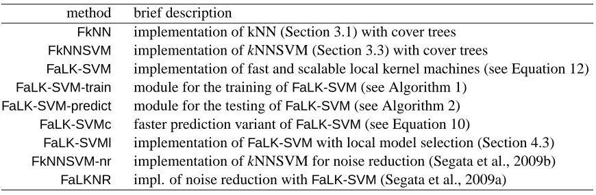
Table 1: Summary for the classifiers developed in the local kernel machine framework and

imple-mented inFaLKM-lib.

in Algorithm 2 (use of cover trees and minimisation of t in Equation 11 are omitted for clearness).

Table 1 summarizes the classifiers discussed in this paper and the modules ofFaLKM-lib.

5. Empirical Analysis

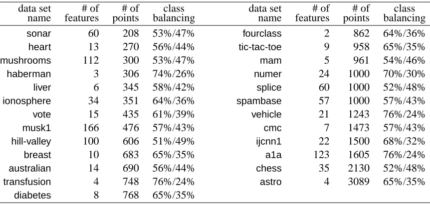
The empirical analysis is organised into three experiments performed with different objectives and using different data sets. Experiment 1 (Section 5.1) has the objective of assessing the

generali-sation performances of FaLK-SVMwith respect to SVM (using LibSVM) and to kNNSVM (using

FkNNSVM) and thus assessing ifFaLK-SVMis more accurate than SVM and if it is a good approxi-mation of kNNSVM. For this experiment we use 25 non-large data sets. Experiment 2 (Section 5.2)

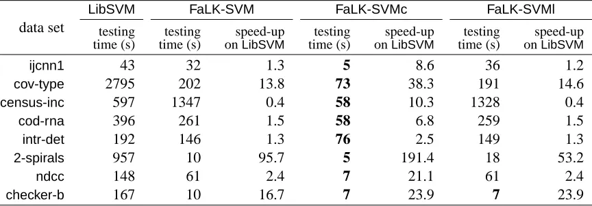
focuses on comparing the classification accuracies and the computational performances of

FaLK-SVM(and its variantsFaLK-SVMcandFaLK-SVMl) with respect to SVM (usingLibSVM) on large

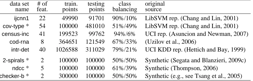
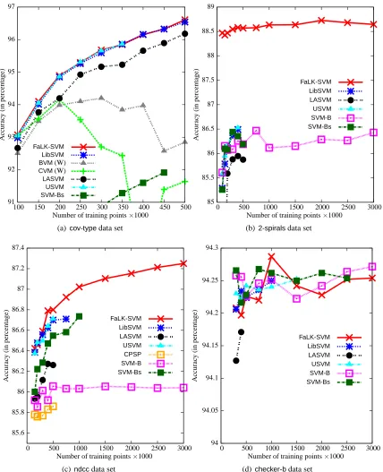
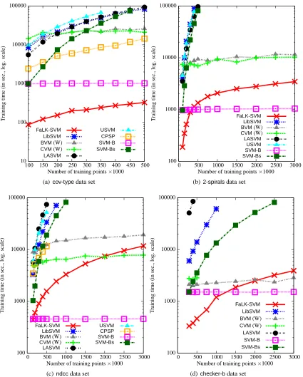
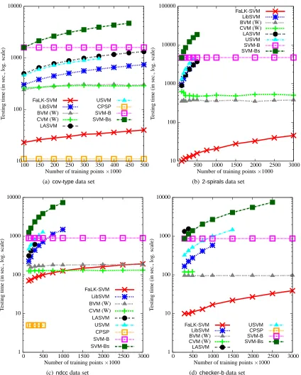
data sets. For this experiment we use 8 data sets with training set cardinalities ranging from about 50k examples to more than 1 million. Experiment 3 (Section 5.3) aims to understand (i) whether FaLK-SVM has better scalability and accuracy performances than LibSVM, a number of

approxi-mated SVM solvers (CVM,BVM,LASVM,CPSPandUSVM) and SVM-bagging and (ii) which are

the computational and accuracy differences betweenFaLK-SVM,FaLK-SVMcandFaLK-SVMl. For

this last experiment we use 4 data sets with increasing training set size up to 3 million examples. The experiments, unless otherwise specified, are carried out on an AMD Athlon 64 X2 Dual Core Processor 5000+, 2600MHz, with 3.56Gb of RAM with Linux operating system.

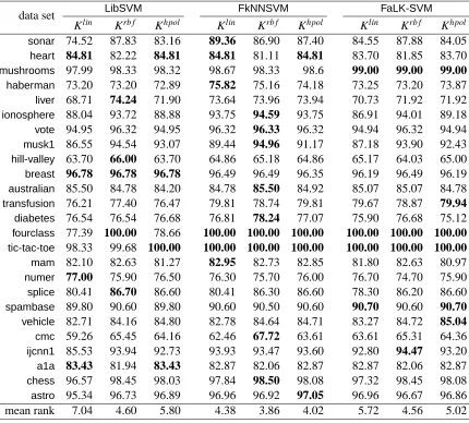
5.1 Experiment 1: Comparison ofFaLK-SVMwithLibSVMandFkNNSVM

In this evaluation we compare SVM (using LibSVM), kNNSVM (using FkNNSVM) and

FaLK-SVMon 25 non-large data sets, with the objective of studying the generalisation performances of

kNNSVM with respect to SVM and the level of approximation introduced by FaLK-SVM to the