Data-Driven Modelling of Natural Gas Dehydrators for Dew Point Determination

(1)

http://www.sciencepublishinggroup.com/j/ogce doi: 10.11648/j.ogce.20170503.11

ISSN: 2376-7669(Print); ISSN: 2376-7677(Online)

Data-Driven Modelling of Natural Gas Dehydrators for Dew

Point Determination

Aniefiok Lawrence Ukpong, Ise Ise Ekpoudom, Eddie Achie Akpan

Department of Electrical/Electronic and Computer Engineering, University of Uyo, Uyo, Nigeria

Email address:

[email protected] (A. L. Ukpong), [email protected] (I. I. Ekpoudom), [email protected] (E. A. Akpan)

To cite this article:

Aniefiok Lawrence Ukpong, Ise Ise Ekpoudom, Eddie Achie Akpan. Data-Driven Modelling of Natural Gas Dehydrators for Dew Point Determination. International Journal of Oil, Gas and Coal Engineering. Vol. 5, No. 3, 2017, pp. 27-33. doi: 10.11648/j.ogce.20170503.11

Received: February 21, 2017; Accepted: March 6, 2017; Published: April 22, 2017

Abstract: The presence of water in natural gas stream is a recurring problem that the oil and gas industry have been dealing

with over the years. Failure to remove water vapor from natural gas stream leads to the formation of hydrates and corrosion of critical facilities. Determination of natural gas dew point which is the temperature at which water vapor condenses out of natural gas is a tricky endeavor, hence there is need to explore modern and more effective ways of determining the dew point. In this research, data driven modeling technique is utilized to generate an expression for the Dew Point of a Natural Gas stream exiting a Molecular Sieve Dehydrator Bed. After data quality analysis, various model structures were utilized for modeling. The Autoregressive Moving Average with exogenous inputs model proved its suitability for predicting the plant output with a highest level of accuracy.

Keywords: Data-Driven Modeling, Dehydrator, Natural Gas, Dew Point

1. Introduction

Determining the precise extent of moisture present in a natural gas well stream prior to carrying out dehydration is of utmost significance, as this will aid and expedite the dehydration procedures and can be beneficial in resolving issues when defects and problems arise in natural gas processing plants [1]. Natural Gas dew point is the temperature at which the free water and other moisture contents of the natural gas begin to condense and drop out of the gas stream [2]. Dew point is the back-bone in the recovery of Natural Gas Liquid (NGL) from a natural gas well stream and must be made as low as possible for efficient production of the Natural Gas Liquid. If the desired natural gas dew point of the NGL recovery plant which is a cryogenic plant is not met, there is a likelihood of hydrate formation and corrosion effects in downstream of the recovery plant [3]. Due to the above mentioned problems, there have been tremendous efforts targeted at lowering and achieving an accurate dew point for natural gas processes. Taking the dynamics of the gas processing plant into consideration, the desired and accurate dew point can be achieved if and only if the natural gas dehydrators are adequately modeled with sufficient number of input and

output. The dew point of the natural gas leaving the dehydrators must be lower than the coldest point of the natural gas liquid production plant; this will prevent the formation of hydrates in the production plant at any point [4].

2. Background Information on

Data-Driven Modelling

(2)

is to aid and guide in the process of deriving a correct and useful mathematical function relating the inputs and output variables [8]. System identification is a tool of data-driven modelling. System identification employs two key techniques in data-driven modelling. The first one is known a black-box modelling specifically useful when your primary interest is in fitting the data regardless of a particular mathematical structure of the model, and is usually a trial-and-error process, where you estimate the parameters of various structures and compare the results. The second is the grey-box modelling which is used when estimating the values of the unknown parameters of your model structure that has already been deduced from physical principles [9].

3. Data Acquisition

The data for this analysis was recorded from a data acquisition device of Natural Gas Liquid (NGL) Molecular Sieve Dehydrator Bed with three input variables, Feed Gas

Flow-rate, Feed Gas Temperature and Feed Gas Pressure; and Output, is the Dew point Temperature. These parameters were chosen because the quantity of moisture present in the natural gas is as dependent on the temperature, pressure and the constituents of the natural gas, thus requiring monitoring of the temperature and pressure of the dehydrator beds [10].

The Pi software used with combination of variable sensors and triplex and delta V monitoring interface in the data acquisition process samples the value of the measured data at 6.00 am (once a day) and log it down for future use. The data obtained from the pi software for the purpose of this project covered a period of two and a half years, ranging from 1st January 2011 to 1st July 2013.

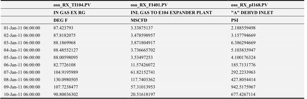
Additionally, the pi software system was accessed and molecular sieve dehydrator bed system trend and logged variables were selected, the period of two and a half years (1st January 2011 to 1st July 2013) was also selected. The data was then down loaded into a Microsoft excel file format. A sample of the data is shown in Table 1.

Table 1. Recorded Data.

oso_RX_TI104.PV oso_RX_FI401.PV oso_RX_pI168.PV IN GAS EX RG INL GAS TO E104 EXPANDER PLANT "A" DEHYD INLET

DEG F MSCFD PSI

01-Jan-11 06:00:00 87.423793 3.33875137 2.188559498

02-Jan-11 06:00:00 87.8182075 3.478598957 3.157794669

03-Jan-11 06:00:00 88.1869968 3.871804917 6.386294669

04-Jan-11 06:00:00 88.48552127 3.736665702 5.103835947

05-Jan-11 06:00:00 88.00598095 3.53497253 4.100176324

06-Jan-11 06:00:00 82.7726108 11.57426072 185.7131776

07-Jan-11 06:00:00 104.9195989 61.82152741 292.2233963

08-Jan-11 06:00:00 130.0980505 117.7403362 427.8054414

09-Jan-11 06:00:00 107.7238477 57.31013953 942.5175967

10-Jan-11 06:00:00 90.80036302 20.51618197 677.4267114

4. Methodology

4.1. Data Pre-Processing

The obtained raw data from the data acquisition device of Natural Gas Liquid (NGL) Molecular Sieve Dehydrator Bed cannot be used for the modelling of the dew point of natural gas exiting the molecular sieve dehydrator instantly as it contains some defects. Such defects include missing values, outliers, offsets and drift and some disturbances [11].

Some Data pre-processing techniques carried out include detection and removal of outliers filtering, detrending, resampling, as well as replacement and removal of missing values.

These pre-processing can be applied to the acquired data to cater for the deficiencies in the data set and make it suitable for the required modelling. Some of these pre-processing techniques will be discussed as they apply to this project. However, some of the pre-processing technique may not be applied to the data set immediately until a data quality analysis is carried out on the obtained data to ascertain their

states [5].

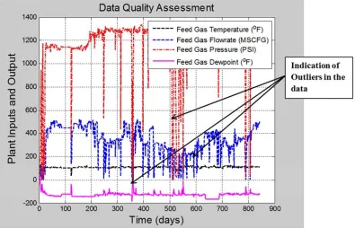
When modeling with data in an off-line situation, plotting of the data must be the first thing to be done so as to determine and examine the defects [12].

4.2. Data Quality Analysis

Prior to commencing the estimation of models from data, the measured data was checked for the presence of any undesirable characteristics by carrying out a time plot of the data. The undesirable characteristics may include the following:

a. Missing data samples b.Drifts and outliers c. Offsets and trends

4.3. Transient Plot of Data

(3)

Figure 1. Time Plotting of Data for Data Quality analysis.

4.4. Handling Missing Data

Certain factors are also responsible for the missing values noticed in the acquired and logged data. These factors include:

a. Shutdown of the NGL extraction plant and other plants that serve as sources of feed gas to the dehydrator beds, either for the purpose of turnaround maintenance or unscheduled shutdown.

b.Failure of either the process variable sensing element or the transmitter.

c. Malfunction of the pi software itself.

d.Network failure within the Oso facility instrument networking and the data acquisition system.

This is one of the pre-processing treatments that can be applied to the data set before carrying out data quality analysis. Once a data file with missing values is loaded into the MATLAB program workspace, MATLAB convert the missing values to NaN which means Not-a-Number without interfering with the structures of the variables containing the missing values

4.5. Data Frequency Response Plots

The spa function was used to estimate frequency response with fixed frequency resolution using spectral analysis before representing this on a bode plot. The algorithm further computes the Fourier transforms of the covariance and the cross-covariance before it finally calculates the frequency-response function and the output noise spectrum of the system. The Bode plots are presented in Figure 2.

Figure 2. Frequency Response Plotting of Feed Gas Pressure to Feed Natural Gas Dew Point.

Frequency response function describes the steady-state response of the dehydrator system to sinusoidal inputs. There are amplitude peaks at certain frequencies for all input-output data combinations which show that the dehydrator will become unsteady at these frequencies. The amplitude peaks at the frequencies of about 0.7 rad/day, 0.5rad/day and 0.4rad/day suggest a possible resonant behaviour (complex poles) for all the input-to-output combination. Moreover, there is rapid phase roll-off at frequency > 0.3rad/day, suggesting the presence of time delays in the data sampling. The frequency response for other pairs show similar characteristics. The step response and impulse response analysis are not presented due to space constraints.

10-2 10-1 100 101

10-2 100

A

m

p

lit

u

d

e

From Feed Gas Pressure to Feed Gas Dewpoint

10-2 10-1 100 101

-400 -300 -200 -100

P

h

a

s

e

(

d

e

g

re

e

s

)

(4)

4.5.1. Decisions

After careful examination of the obtained results of the analysis carried out on the data set, a decision was reached not to detrend, filter and remove the outlier in the data set as these may affect the estimation of the model due to the presence of non-linearity found in the data set but resampling was done to aid in recovery of some lost information.

4.5.2. Resampling

This was the only data pre-processing technique that was carried out on the data sets. In this process, the resampling technique utilizes an antialiasing low pass FIR filter with a 0.08 sampling interval (about 2 hours) to interpolate for the missing information about the dynamics of the system. It is also advisable to decimate the data if it was sampled at much faster rate because such data may contain high-frequency

noise outside the frequency range of the system. For the purpose of model estimation and validation, the resampled data was split into two sets as displayed in Table 2.

Table 2. Splitting of resampled data.

Resampled Data Estimation Validation

Number of Samples 5269 5269

Total 10538

4.6. Modelling Structure

The following model structures were utilized for model cross-validation [5]:

i. Nonlinear Auto-Regressive with exogenous inputs (NARX) model. The structure of this model is written as shown:

= − 1 , … , − , − , … , − − + 1 (1)

ii. Auto-Regressive (AR) Model

= (2) iii.Auto-Regressive with exogenous input(s) (ARX)

Model

= − + (3)

iv.Auto-Regressive Moving Average with exogenous input(s) (ARMAX) Model

= − + (4)

v. Output-Error (OE) Model

= − + (5)

vi.Box-Jenkins (BJ) Model

= − + (6)

vii.State-Space Model

+ = + + (7)

= + + (8)

Where:

is a function that relies on known number of previous

input and output ,

is the number of past output terms used to predict the current output,

is the number of past input terms used to predict the current output and

is the delay from the input to the output, specified as the number of samples.

is the time shift operator dependent on the number of delays in the data samples and the term

models the noise sequence or disturbance inherent in the system.

The model evaluation criteria utilized were Fitness (FIT), Loss Function (V), and Akaike's Final Prediction Error (FPE). Model validation was carried out to examine the models-output plot to see how well the models’ outputs match the measured output in the validation data set.

5. Research Analysis and Results

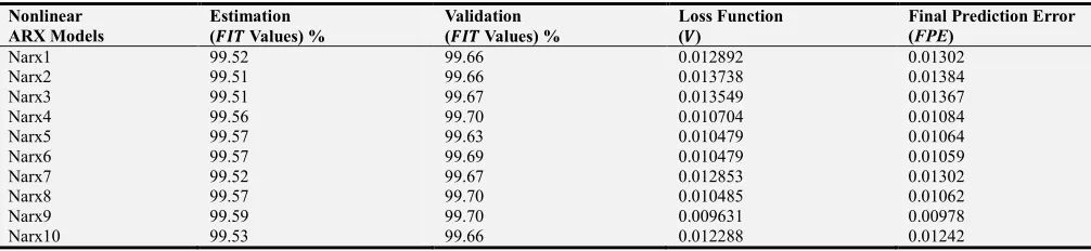
5.1. Model Estimation and Validation Result and Analysis for NARX Models

Table 3 to 7 display the different parameters for various model structures. For each model structure, the model with the highest FIT, lowest Loss Function and lowest Final Prediction Error is chosen and highlighted.

Table 3. NARX Model Evaluation Criteria (FIT, V and FPE Values).

Nonlinear ARX Models

Estimation ("#$ Values) %

Validation ("#$ Values) %

Loss Function (%)

Final Prediction Error (FPE)

Narx1 99.52 99.66 0.012892 0.01302

Narx2 99.51 99.66 0.013738 0.01384

Narx3 99.51 99.67 0.013549 0.01367

Narx4 99.56 99.70 0.010704 0.01084

Narx5 99.57 99.63 0.010479 0.01064

Narx6 99.57 99.69 0.010479 0.01059

Narx7 99.52 99.67 0.012853 0.01302

Narx8 99.57 99.70 0.010485 0.01062

Narx9 99.59 99.70 0.009631 0.00978

(5)

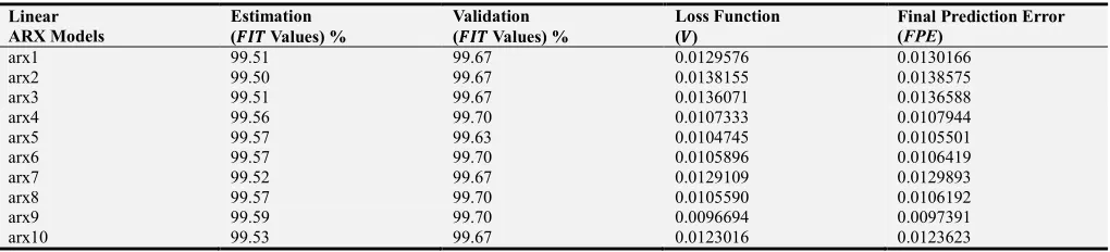
Table 4. Linear ARX Model Evaluation Criteria (FIT, V and FPE Values).

Linear ARX Models

arx1 99.51 99.67 0.0129576 0.0130166

arx2 99.50 99.67 0.0138155 0.0138575

arx3 99.51 99.67 0.0136071 0.0136588

arx4 99.56 99.70 0.0107333 0.0107944

arx5 99.57 99.63 0.0104745 0.0105501

arx6 99.57 99.70 0.0105896 0.0106419

arx7 99.52 99.67 0.0129109 0.0129893

arx8 99.57 99.70 0.0105590 0.0106192

arx9 99.59 99.70 0.0096694 0.0097391

arx10 99.53 99.67 0.0123016 0.0123623

Table 5. State-Space Model Evaluation Criteria (FIT, V and FPE Values).

State Space Models

SSM1 98.56 98.81 0.11680 0.117598

SSM2 98.56 98.81 0.11680 0.117598

SSM3 93.44 90.79 2.42654 2.437590

SSM4 93.44 90.79 2.42654 2.437590

SSM5 93.44 90.79 2.42654 2.437590

SSM6 93.44 90.79 2.42654 2.437590

SSM7 93.44 90.79 2.42654 2.437590

SSM8 98.56 98.81 0.11680 0.117598

SSM9 98.56 98.81 0.11680 0.117598

SSM10 98.56 98.81 0.11680 0.117598

Table 6. Box-Jenkins Model Evaluation Criteria (FIT, V and FPE Values).

Box-Jenkins Models

BJ1 98.54 98.64 0.0766050 0.0770122

BJ2 99.44 99.32 0.0125588 0.0126256

BJ3 99.65 99.75 0.0060331 0.0060812

BJ4 99.19 99.69 0.0102243 0.0102903

BJ5 99.51 99.50 0.0130970 0.0131965

BJ6 99.61 99.72 0.0068007 0.0068628

BJ7 99.39 99.53 39468.600 39783.600

BJ8 99.40 99.74 0.0058195 0.0058593

BJ9 99.43 99.67 0.0132421 0.0133226

BJ10 99.49 99.67 0.0089478 0.0090090

Table 7. ARMAX Model Evaluation Criteria (FIT, V and FPE Values).

Linear ARMAX Models Estimation ("#$ Values) %

ARMX1 99.28 99.34 0.24358500 0.24460400

ARMX2 99.61 99.72 0.00811463 0.00815477

ARMX3 99.58 99.71 0.00930064 0.00933950

ARMX4 99.52 99.70 0.00999814 0.00993388

ARMX5 99.67 99.76 0.0060555 0 0.00610620

ARMX6 99.70 99.78 0.00475646 0.00478904

ARMX7 99.62 99.73 0.00808005 0.00813539

ARMX8 99.68 99.78 0.00483839 0.00487000

ARMX9 99.63 99.74 0.00671544 0.00676910

ARMX10 99.64 99.76 0.00633965 0.00639031

Linear ARX model arx9 has the highest estimated and validated FIT values (of 99.59% and 99.70%) with low V and FPE values of 0.0096694 and 0.0097391. For the state-space models, five models (SSM1, SSM2, SSM8, SSM9and SSM10) show great performance with the same FIT, V and FPE values of 98.56%, 0.11680 and 0.117598. Similarly, the dehydrator bed modeling with Box-Jenkins structure also results in a good model where BJ3 has FIT of 99.65% for estimation and 99.75% for validation with the lowest values

of V and FPE being 0.0060331 and 0.0060812. Finally, linear ARMAX model six depicts a nice performance (FIT = 99.70 and 99.78, V = 0.00475646 and FPE = 0.00478904).

(6)

Table 8. Resultant Models’ Evaluation Criteria (FIT, V and FPE Values).

Model Structures Estimation ("#$ Values) %

Nonlinear ARX 99.59 99.70 0.0096310 0.0097800

Linear ARX 99.59 99.70 0.0096694 0.0097391

State-Space 98.56 98.81 0.1168000 0.1175980

Box-Jenkins 99.65 99.75 0.0060331 0.0060812

Linear ARMAX 99.70 99.78 0.0047564 0.0047890

It can be seen from Table 8 that both nonlinear and linear ARX model structures yields the same results in their level of being able to capture the dehydrator bed dynamics. However, linear ARMAX model seems to perform better than the rest of the other models with the highest fitness of 99.70% for estimation and 99.78% for validation, lowest loss function of 0.0047564 and final prediction error of 0.0047890. This confirms that linear ARMAX model was able to capture the dynamics of the dehydrator bed with the greatest accuracy, given the data sets used in this research, and discomfit the appropriateness of the suggestions offered by the advice

command.

5.2. Selection and Presentation of Dehydrator Bed Model

Model estimation and validation carried out on different types (NARX, ARX, state-space, BJ and ARMAX) of linear model structures prove successful with no failure on the validation data set. Hence, the best estimated model would be selected among the five resultant models. From table 8, the model tagged linear ARMAX produces the best combination of our model validity criteria for estimation and validation data. Therefore, linear ARMAX was selected because it is the model that is seen to have accurately captured the dehydrator bed dynamics. Table 9 highlights the model parameters:

Table 9. Linear ARMAX Model Parameters.

Model Parameters Description

& number of poles of the system 4

&' number of zeros of the system [4 4 4]

&( number of previous error terms on which the current output depends 2

&)

number of input samples that occur before the inputs affect the current output

[10 10 1]

The expression generated by MATLAB for the molecular sieve dehydrator bed is

Discrete-time IDPOLY model:

A(q)y(t) = B(q)u(t) + C(q)e(t) (9) Where:

A(q) = 1 - 2.511 q^-1 + 1.536 q^-2 - 0.1147 q^-3 + 1.475 q^-4 - 2.172 q^-5 + 0.7871 q^-6

B1(q) = -0.01352 q^-10 + 0.01252 q^-11 + 0.01147 q^-12 - 0.01085 q^-13

B2(q) = 0.0001241 q^-10 - 0.0001583 q^-11 B3(q) = -1.653e-005 q^-1

C(q) = 1 + 0.6052 q^-1 - 1.089 q^-2 - 1.088 q^-3 + 0.6042 q^-4 + 0.9976 q^-5

Rearranging the expressions above mathematically, the Auto-Regressive Moving Average with exogenous inputs model structure is expressed as shown below and it is Discrete-time polynomial model as equation 10:

= −0.01352q

012_{+ 0.01252 q}011_{+ 0.01147 q}015_{− 0.01085 q}017

1 − 2.511q01_{+ 1.536q}05_{− 0.1147q}07_{+ 1.475q}09_{− 2.172 q}0:_{+ 0.7871 q}0;u1 t

+ 0.0001241q

012_{− 0.0001583 q}011

1 − 2.511q01_{+ 1.536q}05_{− 0.1147q}07_{+ 1.475q}09_{− 2.172 q}0:_{+ 0.7871 q}0;u2 t

+ −1.653e

0: 01

1 − 2.511q01_{+ 1.536q}05_{− 0.1147q}07_{+ 1.475q}09_{− 2.172 q}0:_{+ 0.7871 q}0;u3 t

+ 1?2.;2:5@

AB_{01.2CD @}AE_01.2CC@AF_{? 2.;295@}AG_{? 2.DDH;@}AI

105.:11@AB_?1.:7;@AE_02.119H@AF_?1.9H:@AG_{0 5.1H5 @}AI_{? 2.HCH1 @}AJ (10) Where is the output (dew-point of the dehydrator feed

gas) at time , 1 is the first input (feed gas temperature), 2

is the second input (feed gas flow-rate) and 3 is the third input (feed gas pressure) and q is the time shift operator. The estimated linear ARMAX model was modeled only for future predictions of the dehydrator dew-point from past and observed inputs and outputs.

6. Conclusion

(7)

The modelling process commenced with the Non-linear Auto-Regressive with eXogenous input (NARX) as suggested by the advice command but on comparison with the linear models, the Autoregressive Moving Average with exogenous inputs model (ARMAX) emerged as the model with the highest fitness of 99.70% for estimation and 99.78% for validation, lowest loss function of 0.0047564 and final prediction error of 0.0047890.

Also achieved, was the investigation of the model’s appropriateness for simulation and prediction purposes. The linear and nonlinear models were confirmed to exhibit low level of accuracy in reproducing the dew-point of the dehydrator bed given sets of measured inputs values. On the contrary, the resultant Autoregressive Moving Average with exogenous inputs model proves its suitability for predicting the plant output with a high level of accuracy.

References

[1] Bahadori, A. "Prediction of Moisture Content of Natural Gases Using Simple Arrhenius-type Function", Central European Journal of Engineering, Vol. 1, Number. 1, 2011, pp. 81-88.

[2] Løkken, T. V., Bersås, A., Christensen, K. O., Nygaard, C. F., and Solbraa, E." Water Content of High Pressure Natural Gas: Data, Prediction and Experience from Field", International Gas Union Research Conference, Oslo Norway, 2008, pp. 12-15.

[3] Gandhidasan, P., Al-Farayedhi, A. A. and Al-Mubarak A. A. "Dehydration of Natural Gas Using Solid Desiccants", Energy, Vol. 26, No. 9, 2001, pp. 855-868.

[4] Mohr, S. H. and Evans, G. M. "Long Term Forecasting of Natural Gas Production", Energy Policy, Vol. 39, No. 9, 2011, pp. 5550-5560.

[5] Solomatine, D., See, L. M., and Abrahart, R. J. “Data-driven Modelling: Concepts, Approaches and Experiences”, Practical Hydroinformatics, Vol. 34, No. 5, 2008, pp. 17-30.

[6] Janes, K. A., and Yaffe, M. B. “Data-driven Modelling of Signal-transduction Networks”, Nature Reviews Molecular Cell Biology, Vol. 7, No. 11, 2006, pp. 820-828.

[7] Friedel, M. J. “A Data-driven Aapproach for Modeling Post-fire Debris-flow Volumes and their Uncertainty”, Environmental Modelling and Software, Vol. 26, No.12, 2011, pp. 1583-1598.

[8] Barbour, S. L. and Krahn, J. “Numerical Modelling: Prediction or Process?”, Geotechnical News, Vol. 22, No.4, 2004, pp. 44-52.

[9] Mathworks (2005). Fuzzy Logic Toolbox.

http://www.mathworks.com/products/fuzzylogic/. Retrieved on the 20th of June 2014. pp. 1 – 22.

[10] Kidnay, A. J. and Parrish, W. R.,. Fundamentals of natural gas processing, CRC Press, Paperback, Florida, 2006.

[11] Lin, H., Thompson, S. M., Serbanescu-Martin, A., Wijmans, J. G., Amo, K. D., Lokhandwala, K. A. and Merkel, T. C. "Dehydration of Natural Gas Using Membranes. Part I: Composite Membranes", Journal of Membrane Science, Vol. 413, No. 19, 2012, pp. 70-81.