8. Stability Control of an Interconnected Power System Using PID Controller

Stability Control of an Interconnected Power System Using PID

Controller

*

Y.V.Naga Sundeep

,

P.NandaKumar

,

Y.Vamsi Babu

,

K.Harshavardhan

*(EEE, P.B.R VITS/JNT University Anantapur,INDIA) ** (EEE, P.B.R VITS/JNT University Anantapur,INDIA) *** (EEE, P.B.R VITS/JNT University Anantapur,INDIA) **** (EEE, P.B.R VITS/JNT University Anantapur,INDIA)

I.

INTRODUCTION

1.1

PID Controller Structure

The PID controllers are most commonly used controllers plant process. They do, present some challenges to control and instrumentation engineers in the aspect of tuningof the gains required for stability and good transient performance. There are several prescriptive rules used in PID tuning[4]. The PID controller encapsulates three of the most important controller structures in a single package. The parallel form of a PID controller has transfer function:

)

sTd

sTi

1

1

(

Kp

sKd

s

Ki

Kp

function

transfer

Controller

PID

=

Gc(s)













Kp=Proportional Gain constant; Ki=Integral Gain constant; Ti=Reset Time constant =Kp/Ki, Kd =Derivative

gain constant; Td = Rate time or derivative time constant.

Fig.1: Structure of PID Controller

The proportional term in the controller generally helps in establishing system stability and improving the transient response while the derivative term is often used when it is necessary to improve the closed loop response speed even further. Conceptually the effect of the derivative term is to feed information on the rate of change of the measured variable into the controller action[1].

ABSTRACT : Maintanence of stability in an interconnected power system is necessary to have good operation ,

e.

Keywords: PID controller, Dynamic response,Interconnected power system, Load Frequency controller

The most important term in the controller is the integrator term that introduces a pole at s = 0 in the forward loop of the process. This makes the compensated1 open loop system (i.e. original system plus PID controller) a type 1 system at least; our knowledge of steady state errors tells us that such systems are required for perfect steady state set-point tracking.

1.2 Overview of Load Frequency Control Schemes

Automatic generation control (AGC) can be defined as, the regulation of power output of controllable generators within a prescribed area in response to change in system frequency, tie-line loading, or a relation of these to each other, to maintain the scheduled system frequency and / or the established interchange with other areas within predetermined limits (Elgerd, 2001). Therefore, a control strategy is needed that not only maintains constancy of frequency and desired tie-power flow but also achieves zero steady state error and inadvertent interchange. Although there is a heap of research papers available in the literature relating AGC problem of power systems. They dealt various aspects of AGC schemes demonstrating the superiority of one scheme over the others. However, there are few notable contributions of the early stages of AGC, which have set the landmarks in the development of AGC schemes [5].

The first attempt in the area of AGC has been to control the frequency of a power system via the governor of the synchronous machine. This technique was subsequently found to be insufficient and a supplementary control was included to the governor with the help of a signal which is directly proportional to the frequency deviation plus it’s integral. This scheme constitutes the classical approach to the AGC of power systems. Cohn has done very early works in this important area of AGC. Concordia et al and Cohn have presented basic important works on tie-line power and frequency control and tie line bias control in interconnected systems [7].

The Current Operational Problems working group has discussed the problems and requirements of the regulation of generation on interconnected power systems in short notes namely, Regulation requirement imposed on operators beyond the considerations of long term planners and Regulation performance criteria, Operating problems of system regulation and factors influencing interconnected operations. Among the various types of load frequency controllers, the most commonly used one is conventional Proportional Integral (PI) controller. The PI controller is very simple for construction, implementation and gives better dynamic response, but their performance is unsatisfied when the complexity of the system increases due to load disturbances or load variations. To overcome this problem, intelligent control techniques are more suitable. Intelligent control techniques are of great help in implementation of AGC in power systems. Today’s power systems are more complex and require operation in uncertain and less structured environment. Consequently, secure, economic and stable operation of a power system requires improved and innovative methods of control. Intelligent control techniques provide a high adaption to changing conditions and have ability to make decisions quickly by processing imprecise information. Some of these techniques are rule based logic programming; model based reasoning, computational approaches like fuzzy sets, artificial neural networks and genetic algorithms.

II. DESIGN OF INTERCONNECTED POWER SYSTEM

The main difference between Load Frequency Control of multi-area system and that of single area system is, the frequency of each area of multi-area system should return to its nominal value and also the net interchange through the tie-line should return to the scheduled values. So a composite measure, called area control error (ACE), is used as the feedback variable. A decentralized controller can be tuned assuming that there is no tie-line exchange power, i.e.∆Ptiei = 0. In this case the local feedback control will be ui = -Ki(s)Bi.∆fi.. Thus load frequency controller for each area can be tuned independently. To illustrate the decentralized PID tuning method, consider a Three-Area power system as shown in Fig.(2).

Fig(2): Three Area Interconnected Power System with Tie-lines

Let area 1, 2, 3 are not identical systems i.e Area-1 consists of non-reheated turbine, Area-2 has reheated turbine and Area-3 has Water or Hydro turbine. Since the Reheat turbines have different stages due to high and low steam pressure, the Reheat turbines are modeled as second-order units. Hydraulic turbines are non-minimum phase units due to the water inertia. In the hydraulic turbine, the water pressure response is opposite to the gate position change at first and recovers after the transient response. Now it is required to tune a decentralized load frequency controller i.e., tune PID controller for[2]

i i psi ti sgi psi ti sgi i

B

)

/R

G

G

G

(1

G

G

G

(s)

P





Plant-1:

Speed Governor Parameters:

Speed governor time constant Tsg1 = 0.08 sec and Speed governor gain constant Ksg =1

Speed governor regulation parameter R1 = 2.4 Hz/pu MW

Non-Reheat Turbine Parameters:

Turbine time constant Tt = 0.3 sec and Turbine gain constant Kt =1

)

s

08

.

0

1

(

1

)

sT

1

(

1

dynamics

ith

Governor w

Speed

=

G









)

s

3

.

0

1

(

1

)

sT

1

(

1

dynamics

with

Turbine

Reheat

-Non

=

G









Plant-2:

Reheat Turbine Parameters:

Turbine time constant Ttr = 0.3 sec and Turbine gain constant Kt =1

Re-heater time constant (Low Pressure) Tlpr = 10 sec

Coefficient of re-heat steam turbine (High Pressure) Khpr = 0.3

)

(

1

s

3

dynamics

with

Turbine

Reheat

=

G





Plant-3:

Speed governor rest time Tsghy = 5.0 sec Transient droop time constant Ttdhy = 28.75 sec = Tsghy (RT /RP )

Main servo time constant TGH = 0.2 sec Water time constant Tw=1.0 sec

Power System parameters:

Rated area capacity Pr = 2000MW, Tie-Line: Ptiemax=200 MW and (δ1- δ2) = 300

Inertia constant H = 5 MW-s/MVA Rated frequency f0 = 60Hz and Di = 8.33x10-3

Power System Gain Constant Kpsi = 120, Power System Time Constant Tps = 2H/Dif0 = 20

Frequency bias constant Bi = 1/Ri + Di puMW/Hz = 0.425

Syn. Co-efficient Tij =

cos

(

)

P

2

r max







P



T12 =T21 = T23 =T32 = 0.377 and T13 =T31 = 0.503

)

s

20

1

(

120

)

sT

1

(

K

dynamics

with

System

Power

=

G









Now the transfer function of all there are represented as

Transfer function of Area-1 = 1 1 1 1 1 1 1 1

B

)

(s)/R

(s)Gps

(s)Gt

Gsg

(1

(s)

(s)Gps

(s)Gt

Gsg



2

.

106

s

46

.

42

2

s

88

.

15

3

s

106.2







Transfer function of Area-2 =

625

.

10

s

38

.

37

2

s

05

.

44

3

s

96

.

15

4

s

)

625

.

10

s

875

.

31

(











Transfer function of Area-3 =

435

.

4

s

66

.

21

2

s

66

.

29

3

s

58

.

16

4

s

435

.

4

s

74

.

17

2

s

174

.

22















III. PID CONTROLLER AND ITS TUNING

In 1942 Ziegler and Nichols, both employees of Taylor Instruments, described simple mathematical procedures, the first and second methods respectively, for tuning PID controllers. These procedures are now accepted as standard in control systems practice. Both techniques make a priori assumptions on the system model, but do not require that these models be specifically known. Ziegler-Nichols formulae for specifying the controllers are based on plant step responses. The Ziegler-Nichols rule is a heuristic PID tuning rule that attempts to produce good values for the three PID gain parameters. Those are Kp - the controller path gain, Ti-

the controller's integrator time constant and Td - the controller's derivative time constant [4]. Recently a new

tuning rule for PID controller was prepared by Ziegler-Nichols called Pessen Integral Rule (PIR) which is a proposed method in this paper. The procedure for tuning a PID controller using Pessen Integral Rule (PIR) is similar to 2nd method of Ziegler-Nichols PID tuning[1,4,6].

The steps for tuning a PID controller using Pessen Integral Rule is as follows:

1. Reduce the integrator and derivative gains to 0.

2. Increase Kp from 0 to some critical value Kp=Kcrat which sustained oscillations occur.

If it does not occur then another method has to be applied.

3. Note the value Kcrand the corresponding period of sustained oscillation, Pcr.

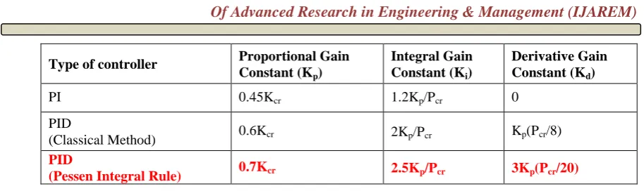
The controller gains are now specified as follows:

Type of controller Proportional Gain Constant (Kp)

Integral Gain Constant (Ki)

Derivative Gain Constant (Kd)

PI 0.45Kcr 1.2Kp/Pcr 0

PID

(Classical Method) 0.6Kcr 2Kp/Pcr Kp(Pcr/8)

PID

(Pessen Integral Rule) 0.7Kcr 2.5Kp/Pcr 3Kp(Pcr/20)

Table 1: Ziegler Nichols – Second Method

Z–N tuning creates “quarter wave decay". This is an acceptable result for some purposes, but not optimal for all applications. The Ziegler-Nichols tuning rule is meant to give PID loops best disturbance rejection. Z–N yields an aggressive gain and overshoot – some applications wish to instead minimize or eliminate overshoot, and for these Z–N is inappropriate.

3.1 Tuning of PID Controller using Pessen Integral Rule:

Case-I: Three area power system with identical turbine in each area

Applying Ziegler Nichols – Second tuning method (R-H Criteria) to plant-1, Critical Gain of the plant Kcr =

5.346, ω = 6.516rad/sec and Critical time constant Pcr = 2π/ω = 0.9643. The controller gains for plant-1are as

follows:

Tuning method Proportional Gain Constant (Kp)

Integral Gain Constant (Ki)

Derivative Gain Constant (Kd)

PID

(Classical Method) 3.2085 6.8622 0.377 PID

(Pessen Integral Rule) 3.7422 9.702 0.5413

Table 2: Kp, Ki & Kd values for Plant-i

Case-II: Three area power system with different turbine in each area

Applying Ziegler Nichols – Second tuning method (R-H Criteria) to plant-1, Critical Gain of the plant Kcr =

5.346, ω = 6.516rad/sec and Critical time constant Pcr = 2π/ω = 0.9643. The controller gains for plant-1are as

follows:

Tuning method Proportional Gain Constant (Kp)

Integral Gain Constant (Ki)

Derivative Gain Constant (Kd)

PID

(Classical Method) 3.2076 6.6527 0.3866 PID

(Pessen Integral Rule) 3.7422 9.702 0.5413

Table 2: Kp, Ki & Kd values for Plant-1

Applying Ziegler Nichols – Second tuning method (R-H Criteria) to plant-2, Critical Gain of the plant Kcr =

13.618, ω = 5.432rad/sec and Critical time constant Pcr = 2π/ω = 1.1567. The controller gains for plant-2are as

follows:

Tuning method Proportional Gain Constant (Kp)

Integral Gain Constant (Ki)

PID(Classical Method) 8.17 14.1264 1.1813

PID (Pessen Integral Rule) 9.5326 20.6 1.654

Table 3: Kp, Ki & Kd values for Plant-2

Similarly, applying Ziegler Nichols – Second tuning method (R-H Criteria) to plant-3, Critical Gain of the plant Kcr = 1.0585, ω = 6.23rad/sec and Critical time constant Pcr = 2π/ω = 1.0085. The controller gains for plant-2are

as follows:

Tuning method Proportional Gain Constant (Kp)

Integral Gain Constant (Ki)

Derivative Gain Constant (Kd)

PID (Classical Method) 0.6351 1.26 0.08

PID (Pessen Integral Rule) 0.741 1.837 0.1121

Table 4: Kp, Ki & Kd values for Plant-3

IV. SIMULATION AND RESULTS

The controller gains for proposed output feedback controller are obtained by Pessen Integral Rule.

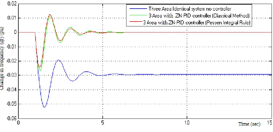
Case-I:

The dynamic response of the system is obtained for 1% step load perturbations in all three areas using MATLAB simulation. The fig.5 shows the change in frequency (df) without and with ZN-PID (classical) & ZN-PID (Pessen Integral Rule) for 1% load perturbation in all three areas. Since the all three area are similar, the change in frequency in all three is same and tie line power variations are zero.

Fig.5 Change in frequency (df) without & with PID for 1% load perturbation in all three areas

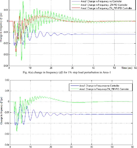
Case-II:

Integral Rule) and change in Tie line power (Ptie) without and with ZN-PID (classical) & ZN-PID (Pessen Integral Rule) for 1% load perturbation in Area-1.

Fig. 6(a).change in frequency (df) for 1% step load perturbation in Area-1

Fig. 6(c).change in Tie line power (dPtie) for 1% step load perturbation in Area-1

The dynamic responses (both variations in frequency and variations in tie line power) for 1% load perturbation in Area-2 are as depicted in figures 7(a), 7(b) and 7(c) without and with PID controllers. The dynamic responses for 1% load perturbation in Area-3 are shown in Figures 8(a), 8(b) and 8(c) without and with PID controllers.

Fig. 7(b).change in frequency (df) for 1% step load perturbation in Area-2

Fig. 8(a).change in frequency (df) for 1% step load perturbation in Area-3

Fig. 8(b).change in frequency (df) for 1% step load perturbation in Area-3

The all above results are summarized as shown in below tables.

Area-i

No Controller ZN-PID

(Pessen Integral Rule Tuning) Steady State

error

Settling time

1st peak over shoots

Steady State error

Settling time

1st peak over shoots

Area-1 -0.0118 55 -0.0217 0 44.2 -0.00943

Area-2 -0.0118 51.57 -0.0376 0 44.35 -0.0106

Area-3 -0.0118 59.8 -0.0531 0 43 -0.0352

Table 5: Comparison between No controller and ZN-PID(Pessen Integral Rule Tuning)

V. CONCLUSION

An attempt has been made to tune a decentralized load frequency controller for a three area interconnected Thermal-Thermal-Hydro Power system incorporating Non-reheated, Reheated and Hydraulic turbine in respective areas. In this paper the proposed controllers are tested and their dynamic responses are compared. Frequency deviations of Area-1, Area-2, Area-3 and Tie line power deviations to 1% step load perturbations in all areas with ZN_PID (Classical) and ZN_PID (Pessen Integral Rule-PIR) controllers have been obtained. It is observed that ZN_PID (Pessen Integral Rule) controller give good dynamic responses that satisfy the requirements of LFC than ZN_PID (Classical). The controller design is simple and similar to ZN_PID (Classical) method.

R

[1]. P. Kundur, “Power System Stability and Control” New York: McGraw-Hill, 2003.

[2]. Wen Tan “Unified Tuning of PID Load Frequency Controller for Power Systems via IMC” IEEE Tran. on Power Systems, Vol. 25, No. 1, pp. 341-350, Feb 2010

[3]. Dingyu Xue, YangQuan Chen, and Derek P. Atherton “Linear Feedback Control", by the Society for Industrial and Applied Mathematics, Unit-6, 2007.

[4]. Brian R Copeland ”The Design of PID Controllers using Ziegler Nichols Tuning” IJETE, pp.1-4, Mar

2008.

[5]. K. P. Singh Parmar S. Majhi, D. P. Kothari,” Optimal Load Frequency Control of an Interconnected Power System” MIT International Journal of Electrical & Inst. Engineering Vol.1, No.1, pp1-5, Jan 2011. [6]. Sigurd Skogestad” Simple analytic rules for model reduction and PID controller tuning ” Journal of Process

Control, Vol.13, pp. 291–309, 2003.

[7]. S.Ohba, H.Ohnishi & S.Iwamoto, “An Advanced LFC Design Considering Parameter Uncertainties in Power Systems,” Proceedings of IEEE conf. on Power Symposium, pp. 630– 635, Sep. 2007.

Bibliography:

Y.V.Naga Sundeepwas born in 1991. He received B. Tech (EEE) degree from JNT University, Anantapur and pursuing M.Tech (Power Electronics) from JNT University, Anantapur.PBR Visvodaya Institute of Technology and Science, Kavali . His research interests are in the areas of Power System Operation & Control, power electronics and Flexible AC Transmission Systems.

P.Nanda Kumarwas born in 1989. He received B. Tech (EEE) degree from SV University, Tirupati . Presently Working as Asst Prof. in P.B.R VITS , Kavali. His research interests are in the areas of Power System Operation & Control and Flexible AC Transmission Systems.