Modeling Macroeconomic Variables Using Principal Component Analysis and Multiple Linear Regression: The Case of Ghana’s Economy

http://www.sciencepublishinggroup.com/j/jbed doi: 10.11648/j.jbed.20200501.11

ISSN: 2637-3866 (Print); ISSN: 2637-3874 (Online)

Modeling Macroeconomic Variables Using Principal

Component Analysis and Multiple Linear Regression: The

Case of Ghana’s Economy

Eyiah-bediako Francis

1

, Bosson-amedenu Senyefia

2, *

, Otoo Joseph

3 1

Department of Statistics, University of Cape Coast, Cape Coast, Ghana

2_{Department of Mathematics and ICT, Holy Child College of Education, Takoradi, Ghana}

3_{Department of Statistics and Actuarial Science, University of Ghana, Legon, Greater Accra, Ghana}

Email address:

*

Corresponding author

To cite this article:

Eyiah-bediako Francis, Bosson-amedenu Senyefia, Otoo Joseph. Modeling Macroeconomic Variables Using Principal Component Analysis and Multiple Linear Regression: The Case of Ghana’s Economy. Journal of Business and Economic Development.

Vol. 5, No. 1, 2020, pp. 1-9. doi: 10.11648/j.jbed.20200501.11

Received: December 25, 2019; Accepted: January 4, 2020; Published: January 13, 2020

Abstract:

The paper sought to model the relationship between GDP and 29 macroeconomic variables in Ghana using the Principal Component Analysis and multiple linear regression. Economic data with 583 data points were collected from January, 1990 through to May, 2018. The KMO statistics was 0.750 and the Bartlett's Test of sphericity statistic obtained for the data was 24807.231 of p-value 0.000. The variables were found to be powerfully correlated with reference to the correlation matrix. Principal Component Analysis was performed to reduce the factors (using orthogonal varimax technique to produce uncorrelated factor structures to help allocate appropriately loadings to factors) to a minimum without compromising the variability of the original data. Seven factors were retained (explained 74% of the overall variation) after using multiple extraction approaches of Scree test, Kaiser Criterion and parallel analysis to avoid over- and under-extraction errors. Regression analysis was performed where component scores were used to develop a relationship with the uncorrelated components and GDP. The component 2 (Closed Economy without Government Activities) explicitly contained seven indicators consisting of consumer price index-Food, Consumer price index-Nonfood, Consumer Price index (overall), Monetary Policy Rate, 91-Days Treasury Bill, 182-Days Treasury Bill, crude oil, and Core Inflation (Adjusted for Energy and Utility). Component 2 was significant and positively related with GDP (B = 0.6, p<0.01). Again, Component 5 (Closed Economy with Government activities) explicitly contained two indicators such as Tax-Equivalent Rate on 28-Days Treasury Bill and Tax-Equivalent Rate on 56-DaysTreasury Bill. Component 5 had a positive and significant impact on GDP (B = 0.386, p<0.01). However, component 4 (monetary economy; B = -3.927, p<0.01), component 6 (B = -0.577, p<0.01) and component 7 (B = -0.256, p<0.01) were negatively related with GDP but were statistically significant. The R-squared value of 0.304 shows that the regression model explains about 30% of the variance. It was recommended for future researchers to consider increasing the number of macroeconomic variables to increase the predictive power of the model.

Keywords:

Principal Component Analysis, Modeling, Macroeconimic Economic Variables, Ghana, Factor Analysis, Eigenvalues, Multiple Linear Regression

1. Introduction

Principal components analysis (PCA) has been extensively applied in diverse fields as a multivariate approach in reducing the dimension of data points so as to facilitate the interpretation and construction of predictive models [1].

Decomposition and dimensional reduction techniques such as Principal component analysis is recommended for a study that involves exploring multidimensional data [2].

analysis. From their results, seventeen variables contributing to GDP were retained in three factors. These three factors derived by the method of PCA were the service factor, agriculture & infrastructure factor, and the fishing & mining factor. In the maximum likelihood method the factors we renamed as service factor, agriculture & infrastructure factor, and education factor.

Hussain et al. (2016), [4] also examined the impact of macroeconomic variables on GDP in Pakistan using multiple regression model. The study found a significant effect on inflation rate, interest rate, and exchange rate on GDP.

A study by Purnamasari et al. (2019), [5] determined the factors capable of affecting learning motivation of students at Yogyakarta State University Postgraduate Program. By the method of Factor analysis, six factors were identified to affect student motivation. These factors were diligence, discipline, discipline and learning frequency, motivation, independence, time management.

A study by Adongo et al. (2018), [6] used PCA to determine the extent of redundant information from correlation matrix. Varimax rotation was applied. Three factors were retained by scree test. The first factors had 6 indicator loadings, the second had one indicator loading, and the third factor had one indicator loading between the nine macroeconomic indicators. They established that PCA method was more robust in comparison with maximum likelihood estimate MLE method. However, the researchers failed to consider varied extraction approaches prior to making decisions on the number of components to retain. This is noteworthy as since the Scree test is known to be highly subjective.

Razak et al. (2015), [7] applied PCA to socioeconomic variables in Asia and found a strong significant and positive correlation between life expectancy at birth and health expenditures, gross national income, good governance, and a healthy life. The study however did not consider the parallel analysis in decision making with regards to the number of components to retain.

Twenefour et al. (2015), [8] in their study sought to identify a yardstick for measuring student performance in a public school in Ghana using PCA. The researchers retained three components using scree test and Kaiser Criterion. The parallel analysis method which has been found to be the most robust method was not incorporated.

The ability of researchers to correctly determine the number of components to retain in PCA has been a major problem confronting researchers. Errors arising from such problems may lead to over-extraction or under-extraction. Field (2005), [9] suggested that if the sample size is more than 250 and the average communality is above 0.6 then one can retain all factors having Eigen values beyond 1 (Kaiser’s criterion). He further suggested for Scree Plot to be used for sample size of at least 300. A study by Scott et al. (1995), [10] reviewed articles that applied PCA (by comparing the three methods such as scree plot, Kaiser Criterion and parallel analysis) from 1987-1993 found that parallel analysis was the most robust method in deciding on the number of

components to retain. Williams (2012), [11] suggested that multiple extraction techniques should be explored before making decisions to retain prospective components.

2. Method

The study examined 30 economic variables (with samples obtained from 583 data points) in Ghana. Data was obtained from the Bank of Ghana (annual reports) panning the years from 1990 through to May of 2018. The analytical methods of PCA and regression analysis were employed.

2.1. Construction of Principal Components

For a random vector, X, with domain ℜm, will have a mean and covariance matrix of µ_X and ∑_X , respectively.

1 2 m 0

λ λ> >⋯>λ > _{for an array of eigenvalues of}

X

∑ , so

that the i-th eigenvalue of ∑_X represents the largest i-th eigenvalue. Suppose a vector α_i denotes the i -th eigenvector of ∑_X corresponding to the i-th eigenvalue of

X

∑ . We wish to derive principal components (PCs) form by

considering the maximization ofvar[α₁TX]=α₁T∑Xα₁, with

respect to α α₁T ₁=1 (a typical optimization problem). The Lagrange multiplier approach is then applied to solve the problem.

To that end,

1 1 1 1 1 1 1

( , ) T X ( T 1)

Lα ϕ =α ∑ α ϕ α α+ −

1 1 1 1

2 X 2 0

L _{α ϕ α}

α

∂ = ∑ _{+ =}

∂ ⇒ Xα1 ϕ α1 1

∑ _{= − ⇒}

1 1 1 1 1

var[αTX]= −ϕ α αT = −ϕ _.

Since −ϕ₁ represent the eigenvalue of ∑_X , with α₁

denoting the respective normalized eigenvector, var[α₁TX] is maximized when α₁ chosen as the initial eigenvector of

X

∑ . To this end, z₁=α₁TX is reffered to as the first PC of

X, with α₁ representing the vector of coefficients for z₁, where var( )z₁ =λ₁.

To get the second PC, z₂ =α₂TX , we shall maximize

2 2 2

var[αTX]=αT∑Xα on condition that z2is not correlated

with z1 _{. But}

1 2

cov(αTX,αTX)=0 ⇒ α1 ∑ α2=0 T

X ⇒

1 2 0

α αT =

, which we will solve by maximizingα₂T∑Xα₂,

on condition thatα α₁T ₂ =0, andα α₂T ₂ =1. We again make use of the Lagrange multiplier approach.

To that end,

2 1 2 2 2 1 1 2 2 2 2

( , , ) T X T ( T 1)

2 1 1 2 2 2

2 _X 2 0

L _{α ϕ α ϕ α}

α

∂ = ∑ _{+ + =}

∂

⇒ 1(2 2 1 1 2 2 2) 0 T

X

α ∑ α +ϕ α + ϕ α = _⇒ ϕ =₁ 0

⇒ ∑Xα2 = −ϕ α2 2 ⇒ 2 2 2 T

X

α ∑ α _{= −}ϕ

.

As −ϕ₂ is the eigenvalue of ∑X , where α2 is the respective normalized eigenvector, we are able to maximize

2

var[αTX] when we select α₂ as the second eigenvector of

X

∑ . As a result, z₂ =α₂TX becomes the second PC of X,

where α₂ represents the vector of coefficients for z₂, and

2 2

var(z )=λ . Per the above results, we can deduce that the i

-th PC zi=αiTX is constructed αi is chosen as the i -th eigenvector of ∑_X , which will then have the variance λ_i. We can conclude by the above results that PCA are the only set of linear functions of original data that are uncorrelated and have orthogonal vectors of coefficients. PCA relies on either covariance matrix or the correlation matrix. The linear combination weights directly originate from combination eigenvectors of correlation matrix or covariance matrix.

Recall that for m variables, the m m× covariance or correlation matrix will contain the following sets:

1 2 p

m eigenvalues {l , l , . . . , l }−

1 2 p

m eigenvectors {e , e , . . . , e }.−

E ach principal component (PC) formed when we considering the values of the elements of the eigenvalues as the weights of the linear combination [6, 12].

Assuming that the k-th eigenvector

(

)

k 1k 2k pk

e = e , e , . . ., e , then the PCs Y , ₁ …, are

produced by

1 11 1 21 2 m1

Y = e X + e X + . . . + e Xm

2 12 1 22 2 m2

Y = e X + e X + . . . + e X ..._m

1m 1 2m 2

Y_m= e X + e X + . . . + e_mmX_m

2.2. Multiple Linear Regressions

The data

1 11 12 1 2 21 22 2 1 2

( ,Y z ,z ,…,z_r), ( ,Y z ,z ,…,z_r),…, ( ,Y z_{n n},z_n ,…,z_nr)

will have the following multiple linear regression model:

0 1 1 2 2 , 1, , ,

i i i r ir i

Y =β +β z +β z + +⋯ β z +ε i= … n

The terms satisfy the following properties:

( )

( )

2

(

)

1.E εi =0; 2.Var εi =σ ; 3.Cov ε εi, j =0,i≠ j

The matrix form of the above data is:

1 0 1 11 1 1 0 1 11 1 1

2 0 1 21 2 2 0 1 21 2 2

0 1 1 0 1 1

r r r r

r r r r

n n r nr n n r nr n

Y z z z z

Y z z z z

Y

Y z z z z

β β β ε β β β ε

β β β ε β β β ε

β β β ε β β β ε

+ + + + + + +            _{+ + + +}   _{+ + +}            =_{ }=_{ }=_{  }+ _         + + + + + + +         ⋯ ⋯ ⋯ ⋯ ⋮ ⋮ ⋮ ⋮ ⋯ ⋯ Or

11 1 0 1

21 2 1 2

1 1 1 1 r r

n nr r n

z z z z Z z z ε β ε β β ε ε β             ₊ _{= +}                 ⋯ ⋯ ⋮ ⋮ ⋱ ⋮ ⋮ ⋮ ⋯ Where;

1 11 1 1 0

2 21 2 2 2

1 1 1 , , , 1 r r

n n nr n r

Y z z

Y z z

Y Z

Y z z

ε β ε β ε β ε β                         =_{ } =_{ } =_{ } =_{ }                 ⋯ ⋯ ⋮ ⋮ ⋮ ⋱ ⋮ ⋮ ⋮ ⋯ .

The error terms are;

( )

( )

( )

2

;

1.E ε =0;and 2.Cov ε =E εεt =σ I

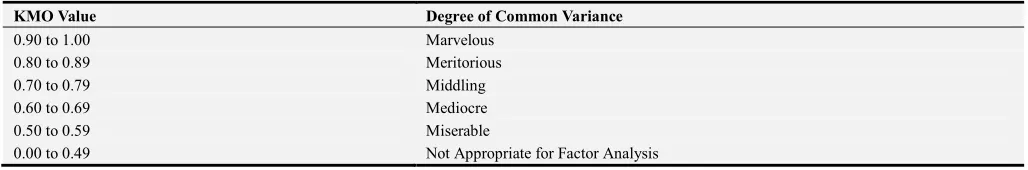
Table 1. Interpretation of the KMO as characterised by Kaiser, Meyer, and Olkin.

KMO Value Degree of Common Variance

0.90 to 1.00 Marvelous

0.80 to 0.89 Meritorious

0.70 to 0.79 Middling

0.60 to 0.69 Mediocre

0.50 to 0.59 Miserable

0.00 to 0.49 Not Appropriate for Factor Analysis

(Schwarz, 2011).

3. Results

William (2010), [11] suggested that the sample size of at least 300 and the sample-variable ratio of 10: 1 are adequate

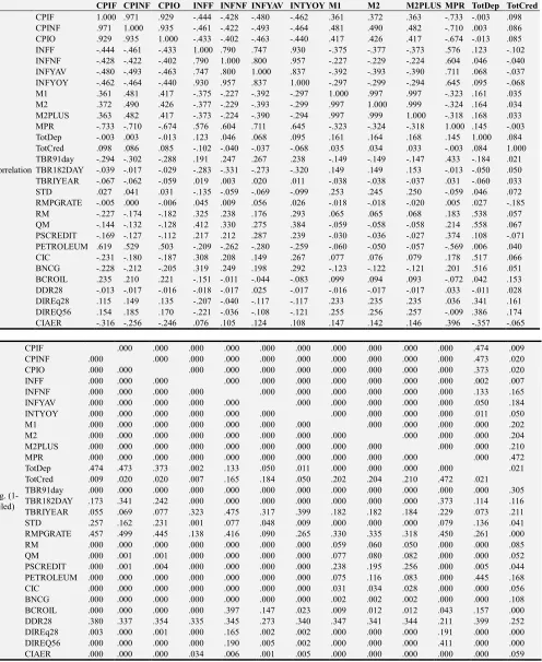
Table 2. Truncated Correlation Matrix.

CPIF CPINF CPIO INFF INFNF INFYAV INTYOY M1 M2 M2PLUS MPR TotDep TotCred

Correlation

CPIF 1.000 .971 .929 -.444 -.428 -.480 -.462 .361 .372 .363 -.733 -.003 .098

CPINF .971 1.000 .935 -.461 -.422 -.493 -.464 .481 .490 .482 -.710 .003 .086

CPIO .929 .935 1.000 -.433 -.402 -.463 -.440 .417 .426 .417 -.674 -.013 .085

INFF -.444 -.461 -.433 1.000 .790 .747 .930 -.375 -.377 -.373 .576 .123 -.102

INFNF -.428 -.422 -.402 .790 1.000 .800 .957 -.227 -.229 -.224 .604 .046 -.040

INFYAV -.480 -.493 -.463 .747 .800 1.000 .837 -.392 -.393 -.390 .711 .068 -.037

INFYOY -.462 -.464 -.440 .930 .957 .837 1.000 -.297 -.299 -.294 .645 .095 -.068

M1 .361 .481 .417 -.375 -.227 -.392 -.297 1.000 .997 .997 -.323 .161 .035

M2 .372 .490 .426 -.377 -.229 -.393 -.299 .997 1.000 .999 -.324 .164 .034

M2PLUS .363 .482 .417 -.373 -.224 -.390 -.294 .997 .999 1.000 -.318 .168 .033

MPR -.733 -.710 -.674 .576 .604 .711 .645 -.323 -.324 -.318 1.000 .145 -.003

TotDep -.003 .003 -.013 .123 .046 .068 .095 .161 .164 .168 .145 1.000 .084

TotCred .098 .086 .085 -.102 -.040 -.037 -.068 .035 .034 .033 -.003 .084 1.000

TBR91day -.294 -.302 -.288 .191 .247 .267 .238 -.149 -.149 -.147 .433 -.184 .021

TBR182DAY -.039 -.017 -.029 -.283 -.331 -.273 -.320 .149 .149 .153 -.013 -.050 .050

TBRIYEAR -.067 -.062 -.059 .019 .003 .020 .011 -.038 -.038 -.037 .031 -.060 .033

STD .027 .041 .031 -.135 -.059 -.069 -.099 .253 .245 .250 -.059 .046 .072

RMPGRATE -.005 .000 -.006 .045 .009 .056 .026 -.018 -.018 -.020 .005 .027 -.185

RM -.227 -.174 -.182 .325 .238 .176 .293 .065 .065 .068 .183 .538 .057

QM -.144 -.132 -.128 .412 .330 .275 .384 -.059 -.058 -.058 .214 .558 .067

PSCREDIT -.169 -.127 -.112 .217 .212 .287 .239 -.030 -.036 -.027 .374 .108 -.071

PETROLEUM .619 .529 .503 -.209 -.262 -.280 -.259 -.060 -.050 -.057 -.569 .006 .040

CIC -.231 -.180 -.187 .308 .208 .149 .267 .077 .076 .079 .178 .517 .066

BNCG -.228 -.212 -.205 .319 .249 .198 .292 -.123 -.122 -.121 .201 .516 .051

BCROIL .235 .210 .221 -.151 -.011 -.044 -.083 .099 .094 .093 -.072 .042 .153

DDR28 -.013 -.017 -.016 -.018 -.017 .025 -.017 -.016 -.017 -.017 .033 -.011 .028

DIREq28 .115 .149 .135 -.207 -.040 -.117 -.117 .233 .235 .235 .036 .341 .161

DIREQ56 .154 .185 .170 -.221 -.036 -.108 -.121 .255 .256 .257 -.009 .386 .174

CIAER -.316 -.256 -.246 .076 .105 .124 .108 .147 .142 .146 .396 -.357 -.065

Sig. (1-tailed)

CPIF .000 .000 .000 .000 .000 .000 .000 .000 .000 .000 .474 .009

CPINF .000 .000 .000 .000 .000 .000 .000 .000 .000 .000 .473 .020

CPIO .000 .000 .000 .000 .000 .000 .000 .000 .000 .000 .373 .020

INFF .000 .000 .000 .000 .000 .000 .000 .000 .000 .000 .002 .007

INFNF .000 .000 .000 .000 .000 .000 .000 .000 .000 .000 .133 .165

INFYAV .000 .000 .000 .000 .000 .000 .000 .000 .000 .000 .050 .184

INTYOY .000 .000 .000 .000 .000 .000 .000 .000 .000 .000 .011 .050

M1 .000 .000 .000 .000 .000 .000 .000 .000 .000 .000 .000 .202

M2 .000 .000 .000 .000 .000 .000 .000 .000 .000 .000 .000 .204

M2PLUS .000 .000 .000 .000 .000 .000 .000 .000 .000 .000 .000 .210

MPR .000 .000 .000 .000 .000 .000 .000 .000 .000 .000 .000 .472

TotDep .474 .473 .373 .002 .133 .050 .011 .000 .000 .000 .000 .021

TotCred .009 .020 .020 .007 .165 .184 .050 .202 .204 .210 .472 .021

TBR91day .000 .000 .000 .000 .000 .000 .000 .000 .000 .000 .000 .000 .305

TBR182DAY .173 .341 .242 .000 .000 .000 .000 .000 .000 .000 .373 .114 .116

TBRIYEAR .055 .069 .077 .323 .475 .317 .399 .182 .182 .184 .229 .073 .211

STD .257 .162 .231 .001 .077 .048 .009 .000 .000 .000 .079 .136 .041

RMPGRATE .457 .499 .445 .138 .416 .090 .265 .330 .335 .318 .450 .261 .000

RM .000 .000 .000 .000 .000 .000 .000 .059 .060 .050 .000 .000 .085

QM .000 .001 .001 .000 .000 .000 .000 .077 .080 .082 .000 .000 .052

PSCREDIT .000 .001 .004 .000 .000 .000 .000 .238 .195 .256 .000 .005 .044

PETROLEUM .000 .000 .000 .000 .000 .000 .000 .075 .116 .083 .000 .445 .168

CIC .000 .000 .000 .000 .000 .000 .000 .031 .034 .028 .000 .000 .056

BNCG .000 .000 .000 .000 .000 .000 .000 .002 .002 .002 .000 .000 .108

BCROIL .000 .000 .000 .000 .397 .147 .023 .009 .012 .012 .043 .157 .000

DDR28 .380 .337 .354 .335 .345 .273 .340 .347 .341 .344 .211 .399 .252

DIREq28 .003 .000 .001 .000 .165 .002 .002 .000 .000 .000 .191 .000 .000

DIREQ56 .000 .000 .000 .000 .190 .005 .002 .000 .000 .000 .411 .000 .000

CIAER .000 .000 .000 .034 .006 .001 .005 .000 .000 .000 .000 .000 .059

Relationship patterns were examined by critical analysis of the respective Pearson correlation coefficient (from the correlation matrix) between all pairs of the economic variables as well as their one-tailed significance of the coefficients. Multicollineality was a problem since the

correlated with each other. A critical look at the correlation matrix (truncated) shows some highly correlated variables such as CPIF and CPIFN, M1 and M2 among others. There was a case of singularity of the data since numerous data sets yielded significance above 0.5 whilst a number of the correlation coefficients were more than 0.9.

Table 3. Kaiser-Meyer-Olkin (KMO) Measure of Sampling Adequacy/Bartlett's Test of Sphericity.

KMO and Bartlett's Test

Kaiser-Meyer-Olkin Measure of Sampling Adequacy. .750

Bartlett's Test of Sphericity

Approx. Chi-Square 24807.231

df 406

Sig. .000

Null Hypothesis: The inter-correlation matrix of the variables is not different from an identity matrix.

Alternate Hypothesis: The inter-correlation matrix of the variables is different from an identity matrix.

Test Results

χ2 = 24807.231; df = 406; p<0.0001 Statistical Decision

The inter-correlation matrix of the variables is significantly different from an identity matrix. In other words, the sample inter-correlation matrix did not come from a population in which the inter-correlation matrix is an identity matrix. The KMO Statistic was 0.750. The degree of common variance among the ten variables is Middling.

In factor analysis, the factors extracted will account for a substantial amount of variance.

Factor analysis is recommended for analysis when the

Bartlett's test of sphericity is statistically significant (≤0.05), and the KMO statistic exceeds 0.6 [14]. Kaiser-Meyer-Olkin Measure of Sampling Adequacy values which are greater than 0.7 by rule of thumb approach is considered a good indication that PCA will be useful for the variables under study (Williams, 2010). The KMO statistics of 0.750 is an indication of the appropriateness of the correlation matrix for component analysis. The Bartlett’s test of Sphericity tests the difference between the correlation matrix for variables and the identity matrix. Bartlett's Test of Sphericity obtained for the data was 24807.231 and p-value was 0.000; an indication of a significant difference which makes it inferable that our correlation matrix for our measured variables is significantly different from an identity matrix which is consistent with the assumption that the matrix should be treated as factorable. This shows that the Bartlett’s test of sphericity is highly sufficient for the data under study.

Table 4. The eigenvalues greater than one of the correlation matrix.

Eigenvalue Total variance (%)

Cumulative Eigenvalue

Cumulative (%)

7.353 25.356 7.353 25.356

4.629 15.961 11.982 41.317

2.963 10.216 14.945 51.533

2.159 7.445 17.104 58.979

1.859 6.411 18.963 58.979

1.4 4.827 20.363 65.389

1.211 3.852 21.574 70.216

1.117 4.176 22.691 74.329

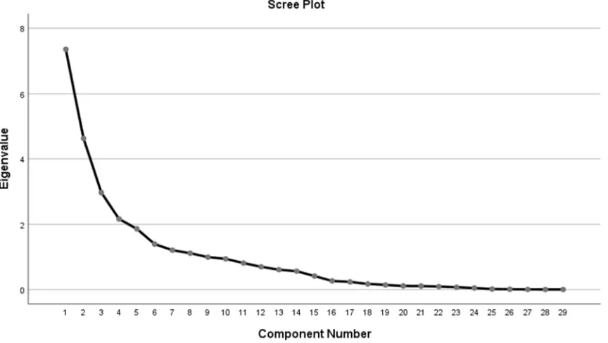
Figure 1. The Scree Plot.

Cattell’s Scree test requires visual analysis of a graphical representation of eigenvalues for point of inflection. The observations above the point of inflection (including the point itself) will inform the number of factors to be retained.

Researcher’s judgment is required in the decision for the number of factors to retain which introduces subjectivity. The subjectivity is reduced for larger sample size [15].

after the fourth principal component

implying that the preceding five principal components can be summarized as being representative of the variables in totality. This is in not in line with the Kaiser criterion (eigenvalue greater than one rule) which extracted 8 factors out of the 29.

Table 5. Parallel Analysis.

Mean Eigenvalue from Eigen values from dataset Eigenvalues retained Parallel Analysis (Kaisor eigen value >1 rule)

1.436368 7.353 7.353

1.377602 4.629 4.629

1.329983 2.963 2.963

1.287357 2.159 2.159

1.252328 1.859 1.859

1.221142 1.400 1.400

1.188662 1.211 1.211

1.162285 1.117

The Kaiser’s eigenvalue >1 rule requires factors with eigenvalues exceeding 1 to be the only ones to be retained.

Parallel analysis (although less applied) has been pointed out by many researchers as the most robust method for retaining factors [15].

Table 5 (second column), the Kaiser’s rule output suggests retaining of 8 factors. The parallel analysis was performed with parameters of 29 economic variables and 583 data points. Percentile Eigen value was set at 95 and the default to generate 100 correlation matrices was maintained. The Eigen values computed from the randomly generated correlation matrices of the parallel analysis were compared with the Eigen values extracted from the data set. The factors which had their Eigen values from the data set exceeding that from that parallel analysis were retained with those failing the threshold considered as spurious as shown in Table 5.To this end, 7 factors were retained. Whereas the Kaiser criterion extracted 8 factors, the parallel analysis suggested retaining only 7 of these out of the 29 variables. To this end, 7 factors were retained for further analysis since the parallel analysis method has been noted as the most robust compared to Scree test and Kaiser criterion (Scott, et al. 1995).

Table 6. Total Variance Explained.

Total Variance Explained Component

Initial Eigenvalues Extraction Sums of Squared Loadings Rotation Sums of Squared Loadings Total % of

Variance Cumulative% Total % of Variance

Cumulative

% Total % of Variance

Cumulative %

1 7.353 25.356 25.356 7.353 25.356 25.356 4.498 15.511 15.511

2 4.629 15.961 41.317 4.629 15.961 41.317 4.253 14.666 30.177

3 2.963 10.216 51.533 2.963 10.216 51.533 4.121 14.210 44.387

4 2.159 7.445 58.979 2.159 7.445 58.979 3.448 11.890 56.277

5 1.859 6.411 65.389 1.859 6.411 65.389 2.106 7.262 63.539

6 1.400 4.827 70.216 1.400 4.827 70.216 1.875 6.464 70.003

7 1.211 4.176 74.392 1.211 4.176 74.392 1.273 4.390 74.392

8 1.117 3.852 78.245

9 .997 3.439 81.684

10 .943 3.253 84.937

11 .816 2.813 87.750

12 .700 2.412 90.162

13 .610 2.103 92.266

14 .563 1.943 94.208

15 .415 1.432 95.640

16 .264 .909 96.549

17 .235 .812 97.360

18 .172 .595 97.955

19 .141 .485 98.440

20 .110 .380 98.820

21 .107 .368 99.188

22 .090 .311 99.499

23 .069 .239 99.738

24 .048 .164 99.902

25 .015 .052 99.954

26 .008 .028 99.982

27 .003 .011 99.993

28 .001 .005 99.998

29 .001 .002 100.000

Extraction Method: Principal Component Analysis.

The first component explains about 25.4% of the total variance. The second component explains about 16% of the overall variance. The third component explains about 10.2% of the total variation and so on and so forth. It can be observed that the first component recorded the greatest

retained variables was about74.4%.

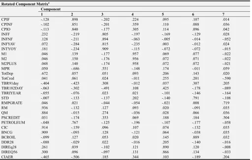
Table 7. Rotated Component Matrixa_.

Rotated Component Matrixa Component

1 2 3 4 5 6 7

CPIF -.128 .898 -.202 .224 .095 .107 .014

CPINF -.102 .851 -.201 .359 .110 .088 .036

CPIO -.113 .840 -.177 .305 .114 .096 .042

INFF .232 -.219 .805 -.197 -.169 -.129 .028

INFNF .128 -.211 .894 -.063 -.005 -.014 -.052

INFYAV .072 -.284 .815 -.235 .003 -.012 .024

INTYOY .181 -.234 .909 -.115 -.072 -.072 -.015

M1 .046 .139 -.177 .957 .069 .077 -.022

M2 .046 .150 -.176 .956 .072 .071 -.022

M2PLUS .048 .140 -.174 .958 .072 .072 -.021

MPR .050 -.686 .551 -.148 .174 -.011 .059

TotDep .672 .057 .051 .093 .206 .143 .020

TotCred .041 .061 .024 -.011 .255 .201 -.590

TBR91day -.404 -.423 .308 -.012 .037 .307 .205

TBR182DAY -.063 -.302 -.491 .108 .425 -.178 -.089

TBRIYEAR -.055 -.076 .023 .021 -.101 -.146 -.164

STD -.007 -.133 -.137 .202 -.140 .791 -.108

RMPGRATE .046 .021 -.044 -.054 -.021 .008 .719

RM .936 -.132 .127 .093 .020 -.091 .035

QM .884 -.015 .274 -.036 .028 .066 .036

PSCREDIT .031 -.174 .353 .069 .188 .184 .504

PETROLEUM -.048 .767 -.125 -.196 -.107 -.177 -.058

CIC .914 -.159 .096 .107 .074 -.132 .035

BNCG .909 -.093 .128 -.121 .064 -.038 .035

BCROIL -.099 .127 .053 .020 .145 .889 .032

DDR28 -.088 -.029 .022 -.016 .205 -.140 -.016

DIREq28 .261 .039 -.102 .121 .890 .120 -.008

DIREQ56 .300 .096 -.097 .131 .866 .134 -.033

CIAER -.465 -.506 .185 .344 .103 -.189 .204

Extraction Method: Principal Component Analysis. Rotation Method: Varimax with Kaiser Normalization. a. Rotation converged in 7 iterations.

Component 1 which is highly correlated (Table 7) with 5 original variables (Total Deposit, Reserve Money, Quasi Money, Consumption index component, and Bank of Ghana Composite Index of Economic Activity (Nominal Growth) was more resembling of a monetary economy.

Component 2 was powerfully correlated (Table 7) with 7 original variables (Consumer price index-food, consumer price index-nonfood, consumer price index overall, Monetary policy rate, crude oil, core inflation adjusted for energy and utility, and 91-dayTreasury Bill was typical of a closed economy without government activity. This is because the indicators are made of mainly investment and consumption factors.

Component 3 which is highly correlated with 5 original variables (Inflation-food, Inflation-nonfood, inflation-average of year, Inflation-year-on-year, 182-Day Treasury

Bill) is a more representative of an inflationary economy. Component 4 is highly correlated with three variables (Narrow Money, Broad Money and Total Liquidity) and a clear case of monetary economy.

Component 5 was highly correlated with 2 original factors (tax-equivalent on treasury bill 28 days, and tax equivalent on Treasury bill 56 days) is a representation of a closed economy with government activity. This is because the indicators are made of investment and government activity (eg. Tax on treasury).

Component 6 has two variables with high correlation (Savings & Time deposits, and International Brent Crude Oil (US$/Barrel) - Monthly Average).

Component 7 has three highly correlated variables (Total Credit, Reserve Money Policy Rate and Private sector credit.

Table 8. Model Summary.

Model Summary

Model R R Square Adjusted R Square Std. Error of the Estimate

1 .551a _{.304 .289 1.97120}

Table 9. ANOVA.

ANOVAa

Model Sum of Squares df Mean Square F Sig.

1

Regression 563.394 7 80.485 20.714 .000b

Residual 1290.026 332 3.886

Total 1853.420 339

a. Dependent Variable: GDP.

b. Predictors: (Constant), REGR factor score 7 for analysis 1, REGR factor score 5 for analysis 1, REGR factor score 1 for analysis 1, REGR factor score 6 for analysis 1, REGR factor score 3 for analysis 1, REGR factor score 2 for analysis 1, REGR factor score 4 for analysis 1.

There was a statistically significant difference among the 7 components.

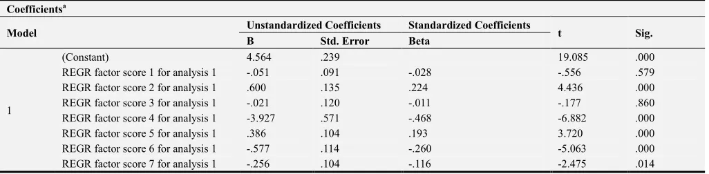
Table 10. Coefficients.

Coefficientsa

Model Unstandardized Coefficients Standardized Coefficients t Sig. B Std. Error Beta

1

(Constant) 4.564 .239 19.085 .000

REGR factor score 1 for analysis 1 -.051 .091 -.028 -.556 .579

REGR factor score 2 for analysis 1 .600 .135 .224 4.436 .000

REGR factor score 3 for analysis 1 -.021 .120 -.011 -.177 .860

REGR factor score 4 for analysis 1 -3.927 .571 -.468 -6.882 .000

REGR factor score 5 for analysis 1 .386 .104 .193 3.720 .000

REGR factor score 6 for analysis 1 -.577 .114 -.260 -5.063 .000

REGR factor score 7 for analysis 1 -.256 .104 -.116 -2.475 .014

a. Dependent Variable: GDP.

The components 2 (closed economy without government activity) and 5 (a closed economy with government activity) were significant and positively related with GDP. However, components 4 (monetary economy), component 6, and 7 are negatively related with GDP and statistically significant. Components 1 (monetary economy) and 3 (inflationary economy) however were not statistically significant and had negative impact on GDP.

4. Conclusion

The paper aimed at modeling the relationship between GDP and 29 macroeconomic variables in Ghana using the PCA and multiple linear regressions methods. Economic data with 583 data points were collected from January, 1990 through to May, 2018. Seven factors were retained (explained 74% of the overall variation) after using multiple extraction approaches of scree test, Kaiser Criterion, and parallel analysis to avoid over- and under-extraction. Regression analysis was performed where component scores were used to develop a relationship with the uncorrelated components and GDP. Closed Economy without Government Activities explicitly contained seven indicators consisting of consumer price index-Food, Consumer price index-Nonfood, Consumer Price index overall, Monetary Policy Rate, 91-DaysTreasury, 182-Days Treasury Bill, crude oil, and Core Inflation (Adjusted for Energy & Utility was significant and positively related with GDP (B = 0.6, p<0.01). Closed Economy with Government activities explicitly contained two indicators such as Equivalent Rate on the 28-DayTreasury Bill and Tax-Equivalent Rate on 56-Day Treasury Bill had a significant

impact on GDP (B = 0.386, p<0.01).

5. Recommendation

Future researchers should consider increasing the number of macroeconomic variables to increase the predictive power of the model.

References

[1] Armeanu D, Lache L. (2018): Application of the Model of Principal Components Analysis on Romanian Insurance Market, Theoretical and Applied Economics.

[2] Fan J, Sun Q, Wen-Xin Z, and Ziwei Z. (2018): Principal component analysis for big data arXiv: 1801.01602v1 [stat. ME].

[3] Syeda F, Muhammad S. and Shah G. A. A (2013). Effects of Macroeconomic Variables on Gross Domestic Product (GDP) in Pakistan. International Conference on Applied Economics (ICOAE) 2013. Procedia Economics and Finance 5 (2013) 703–711.

[4] Hussain A, Hazoor M. Sabir and Kashif M (2016). Impact of macroeconomic variables on GDP: evidence from Pakistan European Journal of Business and Innovation Research Vol. 4, No. 3, pp. 38-52, June 2016.

[6] Adongo F. A, John Amo Jr. L, Chikelu C. J, Osei M, (2018): Principal Component and Factor Analysis of Macroeconomic Indicators, IOSR Journal Of Humanities And Social Science (IOSR-JHSS) Volume 23, Issue 7, Ver. 10 (July. 2018) PP 01-07 e-ISSN: 2279-0837, p-ISSN: 2279-0845. www.iosrjournals.org.

[7] Razzak H, Ali M, (2015): Principal Component Analysis Of Socioeconomic Factors And Their Association With Life Expectancy At Birth In Asia, International Journal of Multidisciplinary Academic Research Vol. 3, No. 1, 2015, ISSN 2309-3218.

[8] Twenefour F. B. K., Nortey E. N. N., Baah, E. M. (2015): Principal Component Analysis of Students Academic Performance International Journal of Business and Social Research, Volume 05, Issue 02, 2015.

[9] Field, A. P. (2005). Discovering statistics using SPSS (2nd edition). London: Sage.

[10] Scott F. B., Gibson, David J., Robertson, Philip A., Pohlmann,

John T. and Fralish, James S. (1995): "Parallel Analysis: a Method for Determining Significant Principal Components." (Feb 1995).

[11] Williams B. (2012): Exploratory factor analysis: A five-step guide for novices. Australasian Journal of Paramedicine Volume 8 | Issue 3.

[12] Hans P. F & Janssens E. (2019). Spurious principal components, Applied Economics Letters, 26: 1, 37-39, DOI: 10.1080/13504851.2018.1433292.

[13] Schwarz J. (2011): Research Methodology: Tools, Applied Data Analysis (with SPSS), Lecture 03: Factor Analysis. [14] Mehmedinovic S. (2017) Fundamentals Of Application Factor

Analysis In Education And Rehabilitation, DOI: 10.21554/hrr.041708.