An improved Active Low Pass Filter

(1)

An improved Active Low Pass Filter

ARUN KUMAR1, RAJIV ASTHANA2, NUTAN LATA3 1

University Department of Physics, Ranchi University, Ranchi.

email: [email protected] 2

Department of Physics, Gossner College, Ranchi.

email: [email protected] 3

Department of Physics, Doranda College, Ranchi.

email: [email protected]

ABSTRACT

A new active low pass filter comprising of two general purpose operational amplifiers (OAs), four resistors and one capacitor is presented. The analytical expressions are obtained and the performance of the proposed circuit is examined in relation to the conventional circuit. Simulation and experimental results are presented which establish the superiority of the proposed low pass filter on the conventional circuit.

Keywords: operational amplifier, Active filter, Active low pass filter.

INTRODUCTION

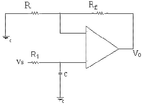
A low pass active filter using operational amplifiers (OA), as shown in Figure1, finds numerous applications in various areas such as instrumentation. A straight forward analysis of the active low pass filter, shown in Figure 1, using 1-pole OA model

஺ఠ

௦ାఠ = ఠ

௦ାఠ (1) gives

0 2

1 1 1 1

1 ( )

( ) 1

s

V

H s G

V s R C G

τ

s R C s

τ

= =

+ + + (2)

with

1

,

1

f

t

R

G

R

ω

τ

=

= +

and ,

where ω₀ is the first-pole frequency, t is the unity gain bandwidth and . Note that =

where

A

₀ is the dc open-loop gain of the op-amp.

(2)

207 Arun Kumar, et al.

Journal of Pure Applied and Industrial Physics Vol.1, Issue of the circuit by minimizing its magni

tude and phase errors. Such efforts have

From Equation (2) it is possible to express the magnitude and phase errors of H(s) as the sum of two components,

0

( ) [1 _H( )]

H s =H +

ε

s

0

( ) ( )

H s H

ε

_φ s

∠ = ∠ +

Where

ε

H( )s and

ε

φ( )s are the magnitude and phase errors respectively, and

0 0

H and H

∠

are the ideal magnitude and phase angles of Equation (2) at s=0. Note that for the low pass filter of Figure 1,

0

H

∠

=0.

Using Equation (2), the new magnitude and phase errors in Equation (3) and (4) may be put in the form

et al., J. Pure Appl. & Ind. Phys. Vol.1 (3), 206-211 (2011)

Journal of Pure Applied and Industrial Physics Vol.1, Issue 3, 30 April, 2011, Pages (162-of the circuit by minimizing its

magni-tude and phase errors. Such efforts have

already been made with success and have been reported in the literature

Figure 1. Conventional low pass filter

From Equation (2) it is possible to express the magnitude and phase errors of H(s) as the sum of two components,

(3) (4) are the magnitude and phase errors respectively, and are the ideal magnitude and phase angles of Equation (2) at s=0. Note that for the low pass filter of Figure 1,

Using Equation (2), the new magnitude and phase errors in Equation (3) and (4) may be

2 2 2 2

1 1

1

( )

(

)

2

H

s

G G

R C

ε

= −

ω

τ

+

1 1

( )s (R C G )

φ

ε

= −

ω

+

τ

From Equations (5) and (6), it follows that the magnitude error is a second order term whereas the phase error is a first order term. In the paper, a new active low pass filter comprising two opamps, three resistors and one capacitor is described. Analytical expressions are obtained and necessary conditions are derived to realize the maximally flat magnitude and phase responses. The feature of this new low pass filter are compared with the conventional low pass filter, using one opamp, three resistors and one capacitor.

211 (2011)

-211)

already been made with success and orted in the literature6-9.

( )

(

)

(5)

(3)

PROPOSED LOW PASS FILTER

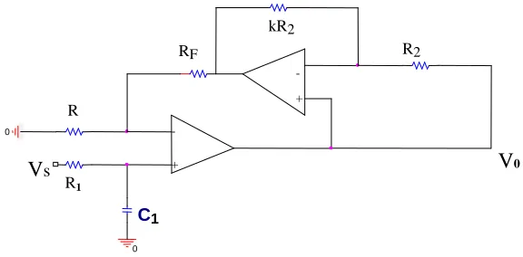
The proposed low pass filter is shown in Figure 2.

Assuming that the opamps are identical, a straight forward analysis of the circuit shown in figure 2, using 1-pole opamp

model, gives the transfer function H(s) in the form

0

2 2 3 2

1 1 1 1 1 1

[1 (1 ) ] ( )

1 ( ) [ (1 ) ] (1 )

s

V G k s

H s

V S R C G s G k R C G s R C G k

τ

+ +

= =

+ + + + + + + (7)

Where _଴_, 1 ோಷ

ோ and τ is the reciprocal of unity gain bandwidth of the opamp. Note that the transfer function in Equation (7) exhibits poles and zeroes in the left-half s-plane and further, that the denominator in Equation (7) satisfies the Routh-Hurwitz stability criterion [10]. Using Equation (7), the maximally flat magnitude response is obtained when

( 2 1) 1 m

k=k = − G− (8)

and maximally flat phase response is achieved for

1

k =k_φ = −G (9)

Using Equation (7)

ε

H( )s and

ε

φ( )s defined by Equations (3) and (4) respectively, under conditions given by Equations (8) and (9) respectively, may be approximately put in the form

(

)

2 3

(

)

4

1 1 1 1

( ) 1

12

H s R C G R C G G k

ω

ε _{= −}_ τ ₊ τ ₊ τ ₊ _ (10)

( )s

φ

ε

=

6ଵଵ ଶଶଷ

(11)

0

C1

R

R1

RF R2

V0 Vs

-+

+

(4)

209 Arun Kumar, et al.

Journal of Pure Applied and Industrial Physics Vol.1, Issue It is seen from equations (10) and

(11) that the magnitude error is a fourth order term whereas the phase error is a third order term, a distinct advantage over the conventional circuit where the magnitude error is a second order term and the phase error is a first order term

SIMULATION AND EXPERIMENTAL RESULTS

A computer simulation of the circuit

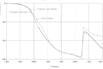
Figure 3: Simulated and experimental magnitude response of circuit in Figure 1 & 2 k=0.242

et al., J. Pure Appl. & Ind. Phys. Vol.1 (3), 206-211 (2011)

Journal of Pure Applied and Industrial Physics Vol.1, Issue 3, 30 April, 2011, Pages (162-It is seen from equations (10) and

(11) that the magnitude error is a fourth order term whereas the phase error is a third order term, a distinct advantage over the conventional circuit where the magnitude cond order term and the phase

SIMULATION AND EXPERIMENTAL

A computer simulation of the circuit

shown in Figure 2 for its magnitude response is plotted in Figure 3 with G=3, k=km=0.242 and upper cut-off frequency 100kHz using 1-pole op-amp model with the parameters listed in Table1. The simulated magnitude response of the conventional low pass filter shown in Figure1 as well as experimental data for circuit shown in Figure 2 are also plotted in Figure 3 to facilitate comparison.

Figure 3: Simulated and experimental magnitude response of circuit in Figure 1 & 2 for dc gain =3 with 211 (2011)

-211)

shown in Figure 2 for its magnitude response is plotted in Figure 3 with G=3, off frequency amp model with the parameters listed in Table1. The simulated magnitude response of the conventional low pass filter shown in Figure1 as well as experimental data for circuit shown in Figure 2 are also plotted in Figure 3 to

(5)

Figure 4: Simulated and Experimental Phase response

It is seen from Figure 3 that the magnitude response of the proposed circuit is much better than the conventional low pass filter circuit. Moreover, the proposed circuit offers an extended frequency range over which the magnitude remains constant, which is a distinct advantage over the conventional circuit. The experimental data plotted in Figure 3 are seen to be in close agreement with the simulated curve for circuit shown in Figure

deviation of the experimental data from the simulated curve may be attributed to the mismatching of the op-amps parameters and their deviation from the parameters used in simulation.

A complete simulation of the circuit shown in Figure 2 using 1

Figure 4: Simulated and Experimental Phase response of circuits of Figure 1 & 2 for gain=3 & k=2

It is seen from Figure 3 that the magnitude response of the proposed circuit is much better than the conventional low pass filter circuit. Moreover, the proposed tended frequency range over which the magnitude remains constant, which is a distinct advantage over the conventional circuit. The experimental data plotted in Figure 3 are seen to be in close agreement with the simulated curve for 2. The minor deviation of the experimental data from the simulated curve may be attributed to the amps parameters and their deviation from the parameters used in A complete simulation of the circuit ing 1-pole op-amp

model for its phase response is plotted in Figure 4 with G = 3 and k = k

simulated phase response of the conventional circuit shown in Figure 1 as well as the experimental data for circuit shown in Figure 2 are also plotted in Fi 4 to facilitate comparison. It is seen from Figure 4 that the phase response of the proposed circuit is much better than the conventional circuit. The experimental data plotted in Figure 4 are seen to be in close agreement with the simulated curve fo circuit shown in Figure 2. The minor deviation of the experimental data with the simulated curve may be attributed to the mismatching of op-amp’s parameters and their deviation from the parameters used in simulation.

of circuits of Figure 1 & 2 for gain=3 & k=2

model for its phase response is plotted in Figure 4 with G = 3 and k = kφ=2. The

(6)

211 Arun Kumar, et al., J. Pure Appl. & Ind. Phys. Vol.1 (3), 206-211 (2011)

Journal of Pure Applied and Industrial Physics Vol.1, Issue 3, 30 April, 2011, Pages (162-211)

Table I: Model Parameters of op-amp

5 0

0

6

1.2 10

9.2 / sec

3.47 10 / sec t

A

rad

ω π

ω

= ×

REFERENCES

1. G. Wilson, ``Compensation of some operational amplifier based RC active network,’’ IEEE Trans. Circuits &

systems, Vol. CAS-23, pp 443-446, (1976).

2. P. Bracket and A. Sedra, ``Active compensation for high frequency effects in op amp circuits with application to active RC filters,’’ IEEE Trans. Circuits

& Systems, Vol. CAS-23, pp 68-73,

(1976).

3. S. Ravichandran and K. R. Rao, ``A novel active compensated scheme for active RC filters,’’ IEEE Proc. , Vol. 68, pp 743-744, 1980.

4. Tey, L.H.; So, P.L.; Chu, Y.C.; ‘Improvement of power quality using adaptive shunt active filter’, Power

Delivery, IEEE Transactions Volume

20, Issue 2, Part 2, Page(s): 1558 – 1568 April (2005).

5. Marques, G.D.; Pires, V.F.; Malinowski, M.; Kazmierkowski, M.;’An Improved Synchronous Reference Frame Method for Active Filters’, EUROCON, 2007. The International Conference on "Computer as a Tool".

6. Anwar A. Khan and Arun Kumar, `A novel noninverting VCVS with reduced magnitude and phase errors,’ IEEE

Trans. on Instrumentation & Measure-ment,’’ Vol. 40, No. 6, pp 919-924

December (1991).

7. Anwar A. Khan and Arun Kumar, `A novel instrumentation amplifier with reduced magnitude and phase errors,’ ’

IEEE Trans. On Instrumentation & Measurement, Vol. 40, No. 6, pp

1035-1038 December (1991).

8. Anwar A. Khan and Arun Kumar, `A novel wide band differenrtial amplifier,’

IEEE Trans. On Instrumentation & Measurement, Vol. 41, No. 4, pp

555-559 August (1992).

9. Anwar A. Khan and Arun Kumar, `Extending the bandwidth of an instrumentation amplifier,’ International

Journal of Electronics, Vol. 74, 1993, pp

643-653.