4. Investigation of intensity laser effects on environment

(1)

Investigation of intensity laser effects on environment

Arash Rezaei

1,*

, Hamid Motavalibashi

2

, Milad Farasat

3

Farhangian university of Isfahan, Isfahan, Iran Iran aircraft Company Isfahan, Isfahan, Iran Farhangian university of Isfahan, Isfahan, Iran

1-

Introduction

In research, especially in the military field, extensive studies have been conducted on guided laser equipment. Use of laser-guided equipment began in America Air Force during the Vietnam War since the 1970s. The first advantage of this type of weapons was confirmed in this war proved in precision destroying targets with relatively small dimensions but with high importance. Today, laser weapons are used much wider for operations against enemy targets armor and protection. The biggest advantage of this type of weaponry is their high precision that can destroy the precise goals with the least amount of ammunition. Another advantage of using these weapons is the possibility of targeting a point precisely for consecutive times that is very efficient to eliminate armor targets. In recent years, military studies and the correct choice of materials for the manufacture of tracker systems pay special attention to laser detectors. Before transmitting a laser beam inside the environment, it is important to identify the effects of the environment on the beam. Molecules and particles such as dust, fog, smoke, steam, and aerosols ,have significant effects on the dispersion, reflection and absorption of laser beams, which themselves contribute to the degradation, deviation, and reduction of laser beam coherence. In this paper, the effects of the environment on the laser beam and the ways to reduce these effects are examined.

2- Discussions

Atmospheric obscurants reduce the performance of sensors by reducing the signal radiation reaching the sensor because of reduced atmosphere transmittance in the sensor wave length response region, increasing noise at the sensor due to scattering of atmosphering radiation or system illuminator energy into the sensor and reducing the signal – to – noise ratio through turbulence induced wave – front degradation.

The three curves indicate a tropical atmosphere with high water vapor content, a subarctic atmosphere, which has a low water vapor content, and a typical us or midlatitude atmosphere, which has a moderate contant . These curves illustrate the effect of water vapor contant on thermal transmittance.

Extinction is defined as the reduction, or attenuation of radiation passing through atmosphere.

Extinction comprise two process: absorption of energy and scattering of energy. In absorption, a photon of radiation is absorbed by an atmosphere molecular or an aerosol particle. In scattering , the direction of the incident radiation is changed by collisions with atmospheric molecular or aerosol particle. Absorption usually dominates scattering at IR and mmw wave length. Scattering is the major factor in visible extinction but may also be important at IR wave length .

Scattering effectiveness is given by the scattering efficiency Q (n , r) which is ratio of the effective scattering cross of a particle of radius r to its geometric cross section as[1, 2] :

(1)

𝑄 𝜆, 𝑟 =

σ

s

πr

2

=

2 r

2

σ

s

θ sinθdθ

π

0

Abstract: In this paper different types of weather conditions which effect laser beam quality are being study. atmospheric conditions such as rain, snow, fog and dust are discussed. Atmospheric turbulence effect on size and intensity of laser beam is described and background optical power relations and received power by receiver are presented. Ground target reflection coefficient and related charts are presented.

(2)

Where

r = particle radius , m

𝜍 = angular scattering cross section , m/sr

𝜃 = scattering angle , rad

If the particle size is much smaller than the radiation wave length , Rayliegh scattering results , and scattering efficiency simplifies to the expression [1] :

(2 )

𝑄 𝜆, 𝑟 =8 3 2𝜋

4𝑟4 𝑛 𝜆 2− 1 2

𝜆4_{𝑛 𝜆}2_{+ 2}2

Where

n(λ) = real part of index of refraction ,r = particle radius , m .

Particale size for several common obscurants are given in tables1 and 2.If the particle size is much larger than the radiation wave length,scattering efficiencycalculated by geometricalscattering.

Table 1the effect of the particles on the order dispersion wave length [1] Effect Distribution type

Radius of particle

Symmetric distribution Rayleigh scattering

less than λ/10

Most distribution Mie scattering

more than λ/10

Most scatting forward Mie scattering

about λ/4

All scatting forward Mie scattering

more than λ

Refraction , reflection , diffraction Light scatting geometry

more than 10 λ

Table 2 particle size distribution and the effect of atmospheric turbulence[1]

mm waves Ir waves

vision waves Diameter of particle

(𝝁m) Particle size

Rayleigh scattering Rayleigh scattering

Rayleigh scattering 10-4

Atmosphere Molecule

Rayleigh scattering Rayleigh scattering

Rayleigh and Mie scattering 10-2 to 10-1

Haze

Rayleigh scattering Mie scattering

Mie and geometric scattering

0.5 t0 100 Fog

2 to 200 Cloud

Mie scattering Geometric scattering

Geometric scattering 102 to 104

Rain

Geometric scattering Geometric scattering

5 × 103_{𝑡𝑜 5 × 10}5

Show

1 Smoke

1 to 100 Dust

According to the table 2 , types of atmospheric particles (steam, aerosols , rain, snow ,…) have different scattering relations.

(3)

The following equation shows the atmosphere transmittance coefficient for steam and molecular particles[1]. ( 3 )

T_m λ = e−Υm λ R

Where

T_m = atmosphere transmittance coefficient for steam and molecular = steam and molecular attenuation coefficient .Υm

R = Path length

The average value of 𝛾 for low humidity ( lower water vaper than 3.5 g /m3 ) in visible spectrum is between 0.4 and 0.7 and for high humidity ( water vaper more than 14 g /m3 ) is about 0.02 .

In the near – infrared range ( between 0.7 and 1.1 ) for low humidity the average value of 𝛾 is about 0.02 and for high humidity is about 0.03 .

The water vapor atmosphere transmittance coefficient within 3 to 5 𝜇𝑚 is specifid in table 3and within 8 to 12

𝜇𝑚 in table 4.

Also according to table 5, the attenuation coefficient for 10.591 wave length and mmw in different humidities.

Table 3Transmission coefficient for water vapor in the atmosphere of moisture and different distances ranging from 3-5 𝝁𝒎[1]

Transmission coefficient for water vapor in the atmosphere of moisture 𝐓_𝐦 𝛌 Along the way in terms km

Temperature ( ℃ ) The

moisture

content 1 3 5 7 10 15

0.47 0.53 0.58 0.62 0.68 0.77 0

10 0.42

0.48 0.53 0.58 0.61 0.74 10 0.38 0.44 0.49 0.53 0.60 0.71 20 0.33 0.39 0.44 0.48 0.55 0.67 30 0.35 0.41 0.47 0.51 0.58 0.70 0

40 0.30

0.36 0.41 46 0.53 0.66 10 0.24 0.30 0.35 0.40 0.47 0.61 20 0.19 0.25 0.30 0.35 0.42 0.56 30 0.30 0.36 0.41 0.46 0.53 0.66 0

70 0.24

0.30 0.35 0.40 0.47 0.61 10 0.18 0.24 0.29 0.34 0.41 0.56 20 0.13 0.18 0.23 0.28 0.36 0.50 30 0.27 0.33 0.39 0.44 0.51 0.64 0

90 0.21

(4)

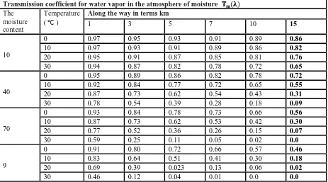
Table 4Transmission coefficient for water vapor in the atmosphere of moisture and different distances ranging from 8-12 𝝁𝒎[1]

Transmission coefficient for water vapor in the atmosphere of moisture 𝐓𝐦 𝛌

Along the way in terms km

Temperature ( ℃ ) The

moisture

content 1 3 5 7 10 15

0.86 0.89 0.91 0.93 0.95 0.97 0 10 0.82 0.86 0.89 0.91 0.93 0.97 10 0.76 0.81 0.85 0.87 0.91 0.95 20 0.65 0.72 0.78 0.82 0.87 0.94 30 0.72 0.78 0.82 0.86 0.89 0.95 0 40 0.55 0.65 0.72 0.77 0.84 0.92 10 0.31 0.43 0.54 0.62 0.73 0.87 20 0.09 0.18 0.28 0.39 0.54 0.78 30 0.56 0.66 0.73 0.78 0.84 0.93 0 70 0.30 0.42 0.53 0.62 0.73 0.87 10 0.07 0.15 0.26 0.36 0.52 0.77 20 0.0 0.02 0.05 0.11 0.25 0.59 30 0.46 0.57 0.66 0.72 0.80 0.91 0

9 0.18

0.30 0.41 0.51 0.64 0.83 10 0.02 0.06 0.13 0.023 0.39 0.69 20 0.0 0.0 0.01 0.04 0.12 0.46 30

Table 5Molecules attenuation coefficient for wavelength 10.591 𝜇𝑚 and millimeter waves atdifferent Humidities[1]

Absolute humidityIn

terms of g/m3 Attenuation coefficient𝚼𝐦In terms of 𝐊𝐦

−۱

10.591 𝝁𝒎 35 GHz 94 GHz

1 0.083 0.018 0.025

3 0.091 0.021 0.043

5 0.109 0.024 0.067

10 0.185 0.032 0.108

15 0.311 0.041 0.154

20 0.383 0.049 0.201

Aerosol (fog , cloud, dust)

The equation below shows the atmosphere transmittance coefficient for aerosols[1]:

Ta λ = e−Υa λ R

whereT_aatmosphere transmittance coefficient Υareduce coefficient of aerosols and R= path length.The avearage

ofΥa in visible spectrum (between 0.4 to 0.7) is:

Υa 0.4 − 0.7μm = 3.912 𝑉 (5)

Where V is visible distance in km

Visible distance is defined as the distance which you can diagnose an object properly by the contrast of l against background by the contrast of 0.02[1]

(5)

Table 6Visible distances for different regions[3]

in IR area for the yag laser:two values will be obtained for aerosols attenuation coefficient one for visible distance more than 0.6 km which is equal to[1]:

Υa1 1.06μm = 10 −0.136 +1.16𝑙𝑜𝑔 3.912 𝑉 (6)

And for a visible distance less than 0.6 km and equal to 0.6 km[1]: Υa2 1.06μm = 3.912 𝑉 (7)

In near-IR range(between 0.7 to 1.1)the average value of Υa is equal to[1]:

Υa 0.7 − 1.1μm = 0.6 3.912 𝑉 (8)

Table7 shows the attenuation coefficient for other wavelength.

Table 7 Attenuation coefficient of suspended particles in the air for wavelength10.591 , 8-12 𝜇𝑚 , 3-5 𝜇𝑚[1]

Particle size _{Attenuation coefficient}_𝚼_𝐚_{in terms of}_𝐊𝐦−۱

10.591 𝝁𝒎 8-12 𝝁𝒎 3-5 𝝁𝒎

May city

Visibility to 2 km 0.16 0.18 0.29

May incident

Visibility to 0.5 km 1.7 2.4 10.1

May rose

Visibility to 0.5 km 8.9 9.0 8.4

Radiation fog forms when the weather cools down until the dew point and advection fog forms when vertical air mixture with different temperatures manufactures until the dew point. In these two types the size of fog particle are different.

0 to 50 meter

Dense dust

50 to 200 meter

Thick dust

200 to 500 meter

The average dust

500 to 1000 meter

Dust weak

1000 to 2000 meter

Low dust

2000 to 4000 meter

Fog

4000 to 10000 meter

May the poor

10000 to 20000 meter

clean Air

20000 to 50000 meter

Very clean air

more than 50000 meter

(6)

Rain:

The following equation defines the atmosphere transmittance coefficient for the precipitation in the air[1].

Tp λ = e−Υp λ R (9)

Where

.Tp= the atmosphere transmittance coefficient for the precipitation in the air

.Υp= the precipitation attenuation coefficient

R=path length

The average value of Υp (in visible spectrum range to thermal wavelength) determines based on the amount of

rainfall for three different types of rainfall. For the drizzle we have[1]:

Υprd Visible − Thermal = 0.51𝑟0.63 (10)

For the widespread we have:

Υ_prw Visible − Thermal = 0.36𝑟0.63₍₁₁₎

And for the thounderstorm we have :

Υprt Visible − Thermal = 0.16𝑟0.63 (12)

Where r = amount of rainfall ( mm per hour(mmph))

Table 8Precipitation

Rainfall intensity Annual rate

Heavy More than 7.7 mm/h

Average 2.5 to 7.7 mm/h

Light Less than 2.5 mm/h

Snowfall:

The atmosphere transmittance coefficient equation for both rainfall and snowfall are the same. The only difference is the attenuation coefficient . the snowfall attenuation coefficient depends on visible distance and equals to[1]:

Υps Visible − Thermal = 3.912 𝑉 (13)

Dust:

The following equation defines the atmosphere transmittance coefficient for dust in the air[1].

Td λ = e−αd λ Cl (14)

Where

.T_d = atmosphere transmittance coefficient for dust in the air ..αd= attenuation coefficient of dust in the air

And cl= path length density by g/m2

Cl achieves from multiplication of upload mass by path length R generally for the a we could write[1] αd λ =≪

𝑄𝜍

𝑀 ≫ (15)

Where:

𝜍 =cross-sectional area of particle Q= the dispersion coefficient M=mass of the particle

The internal bracket is identifier of solid angle average and the external bracket is the identifier of mass distribution average of the particle. For the cl we have:

𝐶𝑙 = 𝐶 𝑟 𝑑𝑙𝑟2

𝑟1 (16)

(7)

𝐶 𝑟 = density at r

. 𝑑𝑙 = longitudinal element of the doped area = length of the doped area 𝑟2−𝑟1

the table 9 shows the dust attenuation coefficient for different wavelength

Table 9Dust in the air attenuation coefficient for different wavelengths[1]

Rainfall intensity Annual rate

Heavy More than 7.7 mm/h

Average 2.5 to 7.7 mm/h

Light Less than 2.5 mm/h

Table 10 shows the masses of different dusts for visible wavelength where visible distance is certain in it.

Table 10Mass loading of dust visible for different distances[1]

Visible distance , Km Mass loading , g/m3

0.2 1.1 × 10−1

0.47 6.9 × 10−2

1 2.1 × 10−2

3.2 5.2 × 10−3

8 2 × 10−3

Smoke:

The following equation defines the atmosphere transmittance coefficient for smoke in the air[1]:

T_s λ = e−αs λ Cl₍₁₆₎

Where

Ts = atmosphere transmittance coefficient for smoke in the air

.αs = attenuation coefficient of smoke in the air,g/m2

And cl = path length of density, g/m2

Cl also defines according to the equation (17)

Table11 shows the amount of attenuation coefficient of types of smoke for different wavelength

Table 11Smoke attenuation coefficient obtained from a variety of sources, to differentwavelengths[1]

Smoke sources

Attenuation coefficient smoke

wavelength in terms of micrometer

0.4 – 0.7 0.7 – 1.2 1.06 3-5 8-12 10.6 35.94 GHz

Fuel

evaporates into

mechanical 6.58 4.59 3.48 0.25 0.02 0.02 0.001

Spray fuel into

(8)

Burning

phosphorus 4.05 1.77 1.37 0.29 0.83 0.38 0.001

Burning zinc

compounds 3.66 2.67 2.28 ]0.19 0.04 0.03 0.001

Coal 6.00 3.50 2.000 0.23 0.05 0.06 0.001

According to the equation 17we could calculate the amount of cl so that l is the length of infected area .then due to the equation16 we could calculate the atmosphere transmittance coefficient for smoke for the all of atmosphere transmittance coefficient in the absence of precipitation we have:

𝑇 λ = T𝑚 λ T𝑎 λ T𝑠 λ T𝑑 λ (17)

And in presence of snowfall or rainfall we have:

𝑇 λ = T𝑚 λ T𝑝 λ T𝑠 λ T𝑑 λ (18)

Light turbulence

The atmospheric turbulence reduces by wavelength enhancement. Atmospheric turbulence causes beam extension beam divagation flashing and fluctuataion in the brightness of the beam[4].

These effect will be describe by radius of beam displacement of the center of beam compatibility or confliction of radiation of the beam.

The scintillation effect causes the reduction of pendulous power average at the receiver aperture. Movement of picture or the blur of the caused turbulence describe by optic function (coherence length) and also wavefront tilt.

The atmospheric turbulence could be considered as a compound of cell with different size and refractive index. These cells move within the beam and cause the effect which is explained at the above. Assuming still and freezed atmosphere the speed and direction of this uniform movement determines by the wind average speed. Based on the size of dominant cell and beam diameter the turbulence cells cause the beam scatterring in different direction. When size of the cell is smaller than the beam diameter refraction and diffraction happens. The beam radiation figure turns into a small ray and the dark area results of int erference of wavefront refraction and diffraction (flicker). Based on the turbulence power ratio each one of the two cases of the above may be observed singly or together. Strehl is the ratio of the average of radiation on the axis with turbulence to the average of radiation on the axis without turbulence .so that the ratio of the beam diameter with turbulence to the beam without turbulence is equal to:

For the long term turbulence cases we have[1] :

𝑆_𝑙 _{= 1 + 𝐷 𝑟} ₀ 2

−1

(19)

And for the short term turbulence if _{𝐷 𝑟} ≤ 3₀ :

𝑆_𝑠1_{= 1 + 0.182 𝐷 𝑟} ₀ 2

−1

(20) And if _{𝐷 𝑟} > 3₀ :

𝑆𝑠2= 1 + 𝐷 𝑟 ₀ 2

− 1.18 𝐷 𝑟 ₀

5 3 −1

(21) Where

D= effective diameter of the laser aperture .𝑆_𝑙= ratio of the long term strehl

.𝑆𝑠= ratio of the short term strehl

And 𝑟₀= coherence length

If the turbulence is uniform we have:

𝑟₀= 0.3325 10−6_𝜆6₅₁₀3_𝐶 𝑛2𝑅

−3

5₍₂₂₎

Where 𝐶𝑛2= constant of the refraction index by 𝑚 −2

3

The amount of 𝐶_𝑛2_{changes between}₁₀−14_{for the weak turbulence}_{6 ∗ 10}−14_{for the medium turbulence and}

6 ∗ 10−13_{for hard turbulence}

(9)

σ_𝐼2_{= 1.24C}

𝑛2 2π _𝜆 7

6

103_𝑅11₆₍₂₃₎

In the spread range or hard turbulence the amount of σ𝐼2 wont be more than 0.5 sigma is by w for the

consubtatial turbulence the amount of σ𝑥2variance of the movement of the center of the picture is equal to:

σ𝑥2 = 1.093C𝑛2𝐹2𝐷 −1

3103_𝑅₍₂₄₎

Where f= focal length of the receiver

The reflection coefficient of ground targets

At first reflection coefficient is reviewed for very important ground targets. Generally natural targets are divided to 5 total categories which three categories of water cloud and snow due to close nature are mentioned in one[5,6].

1- Agricultural land trees bushes and meadows 2- Ground

3- Rocks

4- Water cloud and snow 5- Metals

Received power

To determination of the most range of object location and tracing the lighten object by the laser pulse first of all it's necessary to find the light level in optical receiver sensitive position.

It's specified as well that the angel measurement error is highly dependent to noise signal ratio in output receiver ring.

In more analysis according to table 1-7 geometric characteristic of the laser, the lighten object and the optical receiver are in use to specify the optical power level at the optical reciver input [7].

In analysis, in order to generalize, it's assumed that laser and optical receiver are placed in different places.

Analysis of the power level of the background and reflected optical signal of laser behaives according to the main known equation which is radioscopy. For the background and object it's assumed that scattered reflections are reflected of the Lamberty surfaces.

Also it's assumed that all of the laser beam is on the object which is lighten by laser. Background power

Background optical power which receives from a optical receiver sensitive to location at entrance is equal to [7] :

(10)

.𝐿_𝜆=son radiance spectrum G= geometric factor

.𝑇_𝑅=transference coefficient of optical receiver .𝑇𝐹=transference coefficient of optical filter

And 𝑇_𝑎𝑡=atmosphere transference coefficient

G the geometric factor is obtained from two small area radiative exchange factor and equals to:

G =𝐴𝐷𝐶𝑂𝑆Ө.𝐴𝑅𝐶𝑂𝑆Ө𝑝𝑜

𝑅𝑀2 (26)

Where

.𝐴_𝐷= Quad detector footprint area in background .𝐴_𝑅𝐶𝑂𝑆Ө_𝑝𝑜= The effective area of the photoreceptor

. Ө = The angle between the vector perpendicular to the surface of the object and filed lines between the object and the receiver

.Ө_𝑝𝑜= The angle between the vector perpendicular to the surface receptor filed with the line between the object and the receiver

.𝑅𝑀= The distance between the object and the photoreceptor

In cases where tracking and positioning is good, The photoreceptor is always face to the object so Ө𝑝𝑜 = 0

For the whole radiance of the sun𝐿𝜆 which caused by a diffuse reflector we have:

𝑇𝑎𝑡 = 𝑒−𝛶𝑅𝑀 (27)

Where

= the whole of the sun .𝐸_𝜆

And.𝜌_𝐵= background reflect

The amount of 𝐸𝜆 per wavelength can be obtained from standard charts

.𝑇_𝑎𝑡atmospheric transfer coefficient is obtained from the following relationship comes to

𝑇_𝑎𝑡 = 𝑒−𝛶𝑅𝑀₍₂₈₎

Where

. 𝛶=Atmospheric extinction coefficient.

The back ground power that obtained from equation(25),when combined with equations (26) and (27) has to be obtained as follows.

Where

The whole bandwidth Optical Filter.∆_𝜆=

. 𝛽= photoreceptor visibility range Diameter optical receiver.𝐷𝑝𝑜 =

Signal power

P_S the optical signal received by the laser radiation reflected from the object is lightened with a laser when the laser beam cross-sectional area of the object is smaller than, equals to:

𝑃_𝑆= 𝐿_𝑇𝐴_𝑇𝛺_𝐷𝑇_𝑅𝑇_𝐹𝑒−𝛶𝑅𝑀_{𝐶𝑂𝑆Ө}₍₂₉₎

Where

. .𝐿𝑇=Spectrum reflected from the object

.𝐴_𝑇=The area of the laser spot on the object

And 𝛺𝐷in accordance with Figure 3-7 angle created by the opening of an optical receiver

.𝐿𝑇spectrum is [7-9]

𝐿𝑇=

4𝑃𝐿𝑇𝑇𝜂 𝜌𝑇𝑒−𝛶 𝑅𝐿𝐶𝑂𝑆Ө𝐿

𝜋2_𝛽

𝑇2𝑅𝐿2 (30)

Where

. 𝑃_𝐿= peak power laser

.𝑇_𝑇=transmission coefficient of light

η=efficiency of collection optical transmission .𝜌𝑇=target reflection coefficient

(11)

and 𝑅_𝐿=distance between the laser and the object

.𝐴_𝑇 area of the laser spot on the object of value follow below

𝐴_𝑇 = 𝜋𝑅𝐿2𝛽𝑇2

4𝐶𝑂𝑆Ө𝐿 (31)

And for𝛺_𝐷angle we have:

𝛺_𝐷≈𝜋𝐷𝑝𝑜2

4𝑅_𝑀2 (32)

By combining equations (31) to (33) with equation (30), we finally have for the 𝑃𝑆

𝑃_𝑆=𝐷𝑝𝑜2

4𝑅_𝑀2 𝑃𝐿𝜌𝑇𝑇𝑇η𝑇𝑅𝑇𝐹𝑒

−𝛶 𝑅𝐿 + 𝑅𝑀 _{𝐶𝑂𝑆Ө}₍₃₃₎

Conclusion

According to the formula of laser attenuation by atmospheric conditions such as temperature, humidity, dust, rain, snow polished and smoke and ... which are dependent to the laser wavelength and the distance and the light intensity in order to minimize the laser must:

1- reduse the target distance

2-increase the incident laser beam intensity

3-increaase the Selective laser wavelength because the more higher frequency, the more attenuation efficiency and Conversely is the same situation

4- The purpose of reflecting surface so that the reflection coefficient is higher, For example, hitting a building is better that the laser to hit on smooth surfaces such as metallic windows.

Reference

[1]. DEPARTMENT OF DEFENSE HANDBOOK WASHINGTON DC,Quantitative Description of Obscuration Factors for Electro-Optical and Millimeter Wave System,DOD HDBK-178,(1986).

[2]. M.Pendley, Air Warfare Battlelab Initiative for Stabilized Portable Optical Target Tracking Receiver , International Command and Control Reserch and Technology Symposium the Future of C2, 10𝑡ℎ_edition,

(2004).

[3] Henrik Andersson, Position Sensitive Detectors-Device Technology and Application in Spectroscopy, ISSN 1652-893X,Mid Sweden University Doctoral Thesis 48,ISBN 978-91-85317-91-2,5-25, (2008). [4] Gerald.C.Holst, CCD ARRAYS,CAMERAS and DISPLAYS, 2𝑡ℎ_{edition , SPIE Optical Engineering}

Press, Washington USA, (1998).

[5] K.C.Bahuguna, Prabhat Sharma,N.S.Vasan,S.P.Gaba,Laser Range Sensors, Defence Science Journal, Vol. 57, No. 6, pp. 881-890, (2007).

[6] Department of defense handbook, range laser safety, mil-hdbk-828B, 2𝑡ℎ_{edition,10-35 , (2011).}

[7] Zarko P.Barbaric,Lazo M.Manojlovic,Optimization of Optical Receiver Parameters for Pulsed Laser Tracking Systems, IEEE Transactions on instrumentation and measurement, vol. 58, NO. 3,19-27, MARCH 2009.

[8] Gerald.C.Holst, Electro-optical imaging system performance, 2𝑡ℎ_{edition , SPIE Optical Engineering}

Press, Washington USA,2000.