R E S E A R C H
Open Access
Solving singular second-orderinitial/boundary
value problems in reproducing kernel
Hilbert space
Er Gao
*, Songhe Song and Xinjian Zhang
* Correspondence: gao. [email protected]
Department of Mathematics and Systems Science, College of Science, National University of Defense Technology, Changsha 410073, China
Abstract
In this paper, we presents a reproducing kernel method for computing singular second-order initial/boundary value problems (IBVPs). This method could deal with much more general IBVPs than the ones could do, which are given by the previous researchers. According to our work, in the first step, the analytical solution of IBVPs is represented in the RKHS which we constructs. Then, the analytic approximation is exhibited in this RKHS. Finally, then-term approximation is proved to converge to the analytical solution. Some numerical examples are displayed to demonstrate the validity and applicability of the present method. The results obtained by using the method indicate the method is simple and effective.
Mathematics Subject Classification (2000)35A24, 46E20, 47B32.
1. Introduction
Initial and boundary value problems of ordinary differential equations play an impor-tant role in many fields. Various applications of boundary to physical, biological, che-mical, and other branches of applied mathematics are well documented in the literature. The main idea of this paper is to present a new algorithm for computing the solutions of singular second-order initial/boundary value problems (IBVPs) of the form:
⎧ ⎨ ⎩
p(x)u(x) +q(x)u(x) +r(x)u(x) =F(x,u),
a1u(0) +b1u(0) +c1u(1) = 0,
a2u(1) +b2u(1) +c2u(0) = 0,
(1:1)
where u(x)∈W23[0, 1], for xÎ [0, 1],p≠0,p(x), q(x),r(x)Î C[0, 1].a1, b1,c1, a2, b2,c2 arc real constants and satisfy thata1 u(0) +b1 u’(0) +c1 u (1) and a2 u(1) + b2u’(1) +c2u’(0) are linear independent. F(x,u) is continuous.
Remark1.1. We find that if
b1=c1=b2=c2= 0, a1= 0, a2= 0, (1:2)
the problems are two-point BVPs; if
b1=c1=a2=b2= 0, a1= 0, c2= 0, (1:3)
the problems are initial value problems; if
b1=a2= 0,a1=c1= 0,b2=c2= 0, (1:4)
the problems are periodic BVPs; if
b1=a2= 0, a1=−c1= 0, b2=−c2= 0, (1:5)
the problems are anti-periodic BVPs.
Such problems have been investigated in many researches. Specially, the existence and uniqueness of the solution of (1.1) have been discussed in [1-5]. And in recent years, there are also a large number of special-purpose methods are proposed to pro-vide accurate numerical solutions of the special form of (1.1), such as collocation methods [6], finite-element methods [7], Galerkin-wavelet methods [8], variational iteration method [9], spectral methods [10], finite difference methods [11], etc.
On the other hands, reproducing kernel theory has important applications in numer-ical analysis, differential equation, probability and statistics, machine learning and pre-cessing image. Recently, using the reproducing kernel method, Cui and Geng [12-16] have make much effort to solve some special boundary value problems.
According to our method, which is presented in this paper, some reproducing kernel Hilbert spaces have been presented in the first step. And in the second step, the homo-geneous IBVPs is deal with in the RKHS. Finally, one analytic approximation of the solutions of the second-order BVPs is given by reproducing kernel method under the assumption that the solution to (1.1) is unique.
2. Some RKHS
In this section, we will introduce the RKHS W1
2[0, 1] andW23[0, 1]. Then we will
con-struct a RKHS H32[0, 1], in which every function satisfies the boundary condition of (1.1).
2.1. The RKHS W1 2[0, 1]
Inner space W1
2[0, 1] is defined as W21[0, 1] ={u(x)|u is absolutely continuous real
valued functions,u’Î L2[0, 1]}. The inner product in W1
2[0, 1] is given by
(f,h)W1
2 =f(0)h(0) + 1
0
f(t)h(t)dt, f,h∈W21[0, 1] (2:1)
and the norm ||u||W1
2 is denoted by ||u||W21 =
(u,u)W1
2. From [17,18], W 1
2[0, 1] is a
reproducing kernel Hilbert space and the reproducing kernel is
K1(t,s) = 1 + min{t,s} (2:2)
2.2. The RKHS W3 2[0, 1]
Inner space W3
2[0, 1] is defined as W23[0, 1] ={u(x)|u,u,u is absolutely continuous real valued functions, u"’Î L2[0, 1]}.
From [15,17-19], it is clear that W3
Zhang and Lu [18] and Long and Zhang [19] give us a clue to relate the inner pro-duct with the boundary conditions (1.1). SetL=D3, and
⎧ ⎨ ⎩
γ1f =a1f(0) +b1f(0) +c1f(1),
γ2f =a2f(1) +b2f(1) +c2f(0),
γ3f =a3f(0) +b3f(0) +c3f(0),
(2:3)
wherea3,b3,c3 is random but satisfying thatg3is linearly independent ofg1 andg2.
It is easy to know that g1,g2,g3are linearly independent inKer L. Then from [18,19],
it is easy to know one of the inner products of W3 2[0, 1]
(f,h)W3 2 =
3
i=1
γifγih+ 1
0
f(t)h(t)dt, f,h∈W23[0, 1] (2:4)
and its corresponding reproducing kernelK2(t, s).
2.3. The RKHS H3 2[0, 1]
Inner space H3
2[0, 1] is defined as H32[0, 1] ={u(x)|u,u,u are absolutely continuous real valued functions, u"’ Î L2[0, 1], and, a1 u(0) + b1 u’(0) + c1 u(1) = 0,a2 u(1) + b2u’(1) +c2u’(0) = 0}.
It is clear that H3
2[0, 1] is the complete subspace of W23[0, 1], so H32[0, 1] is a
RKHS. IfP, which is the orthogonal projection from W3
2[0, 1] to H32[0, 1], is found,
we can get the reproducing kernel of H3
2[0, 1] obviously. Under the assumptions of
Section 2, note
Pf(t) = (γ3f)e3(t) + 1
0
G(t,τ)·f(τ)dτ, ∀f ∈W23[0, 1] (2:5)
Theorem 2.1. Under the assumptions above, P is the orthogonal projection from H32[0, 1]to H23[0, 1].
Proof. For all f ∈W3
2[0, 1], We have
(γ1(Pf))(t) = (γ2(Pf))(t) = 0
That means Pf ∈H3
2[0, 1]. At the same time, for any f,h∈W23[0, 1]
(Pf,h) =
⎛
⎝(γ3f)e3(t) + 1
0
G(t,τ)·Lf(τ) dτ,h
⎞ ⎠
= (γ3f)(γ3h) + 1 0 ⎛ ⎝L 1 0
G(t,τ)·Lf(τ)dτ
⎞ ⎠·Lh(t) dt
= (γ3f)(γ3h) + 1
0
Lf(t)·Lh(t) dt
(f,Ph) =
⎛
⎝f, (γ3h)e3(t) + 1
0
G(t,τ)·Lh(τ) dτ ⎞ ⎠
= (γ3f)(γ3h) + 1
0 Lf(t)·L
1
0
G(t,τ)·Lh(τ) dτdt
= (γ3f)(γ3h) + 1
0
P is self-conjugate. And
P(Pf) =P
⎛
⎝(γ3f)e3(t) + 1
0
G(t,τ)·Lf(τ)dτ ⎞ ⎠
= (γ3f)e3(t) + 1
0
G(t,τ)·L
⎛
⎝(γ3f)e3(τ) + 1
0
G(τ,s)·Lf(s)ds
⎞ ⎠, dτ
= (γ3f)e3(t) + 1
0
G(t,τ)·Lf(τ) dτ
=Pf
P is idempotent.
SoP is the orthogonal projection from W3
2[0, 1] to H32[0, 1]. The proof of the Theorem 2.1 is complete.
Now, H3
2[0, 1] is a RKHS if endowed the inner product with the inner product
below
(f,h)H3
2 =γ3fγ3h+ 1
0
f(t)·h(t) dt (2:6)
and the corresponding reproducing kernelK3(t,s) is given in Appendix 4.
3. The reproducing kernel method
In this section, the representation of analytical solution of (1.1) is given in the reprodu-cing kernel space H32[0, 1].
Note Lu = p(x)u”(x) + q(x)u’(x) + r(x)u(x) in (1.1). It is clear that
L:H23[0, 1]→W21[0, 1] is a bounded linear operator.
Puti(x) =K1(xi,x),Ψi(x) =L*i(x), whereL* is the adjoint operator of L. Then
i(x) = (L∗ϕi(y),K3(x,y)) = (ϕi(y),LyK3(x,y))
= (LyK3(x,y),ϕi(x)) =LyK3(x,y)|y=xi
(3:1)
Lemma 3.1. Under the assumptions above, if {xi}∞i=1is dense on [0, 1] then {i(x)}∞i=1is the complete basis H32[0, 1].
The orthogonal system {i(x)}∞i=1 of H23[0, 1] can be derived from Gram-Schmidt
orthogonalization process of {i(x)}∞i=1, and
i(x) = i
j=1
βijj(x).
Then
Theorem 3.1. If {xi}∞i=1is dense on[0, 1]and the solution of(1.1)is unique, the
solu-tion can be expressed in the form
u(x) = ∞
i=1 i
k=1
Proof. From Lemma 3.1,{i(x)}∞i=1 is the complete system ofH32[0, 1]. Hence we have
u(x) = ∞
i=1
(u(x),i(x))i(x) = ∞ i=1 i k=1
βik(u(x),i(x))i(x)
= ∞ i=1 i k=1
βik(u(x),L∗ϕk(x))i(x) = ∞ i=1 i k=1
βik(Lu(x),ϕk(x))i(x)
= ∞ i=1 i k=1
βik(F(x,u(x)),ϕk(x))i(x) = ∞ i=1 i k=1
βikF(xk,u(xk))i(x)
and the proof is complete.
The approximate solution of the (1.1) is
un(x) = n i=1 i k=1
βikF(xk,u(xk))i(x) (3:3)
If (1.1) is linear, that is F(x,u(x)) = F(x), then the approximate solution of (1.1) can be obtained directly from (3.3). Else, the approximate process could be modified into the following form:
⎧ ⎨ ⎩
u0(x) = 0
un+1(x) = n+1
i=1
Bii(x) (3:4)
where Bi= i k=1
βikF(xk,un(xk)).
Next, the convergence of un(x) will be proved.
Lemma 3.2. There exists a constant M, satisfied |u(x)| ≤M||u||H3
2, for all
u(x)∈H3 2[0, 1].
Proof. For allxÎ [0, 1] and u∈H3
2[0, 1], there are
|u(x)|=|(u(·),K3(·,x))| ≤ ||K3(·,x)||H3
2· ||u||H23.
Since K3(·,x)∈H32[0, 1], note
M= max
x∈[0,1]||K3(·,x)||H 3 2.
That is,
|u(x)| ≤M||u||H3 2
.
By Lemma 3.2, it is easy to obtain the following lemma.
Lemma 3.3.If un||·||→ ¯u(n→ ∞), ||un||is bounded, xn® y(n® ∞)and F(x,u(x))is
continuous, then F(xn,un−1(xn))→F(y,u¯(y)).
Theorem 3.2. Suppose that ||un || is bounded in (3.3) and (1.1) has a unique
solution. If {xi}∞i=1is dense on[0, 1],then the n-term approximate solution un(x)derived
from the above method converges to the analytical solution u(x)of(1.1).
From (3.4), we infer that
un+1(x) =un(x) +Bn+1n+1(x).
The orthonormality of {i}∞i=1 yield that
||un+1||2=||un||2+ (Bn+1)2=· · ·= n+1
i=1 (Bi)2.
That means ||un+1||≥ ||un||. Due to the condition that ||un|| is bounded, ||un|| is
convergent and there exists a constantℓsuch that
∞
i=1
(Bi)2=.
Ifm>n, then
||um−un||2=||um−um−1+um−1−um−2+· · ·+un+1−un||2.
In view of (um-um-1)⊥(um-1-um-2)⊥···⊥(un+1-un), it follows that
||um−un||2=||um−um−1||2+||um−1−um−2||2+· · ·+||un+1−un||2
= m
i=n+1
(Bi)2→0 as n→ ∞
The completeness of H3
2[0, 1] shows thatun®ūasn®∞in the sense of || · ||H3 2.
Secondly, we will prove thatūis the solution of (1.1). Taking limits in (3.2), we get
¯
u(x) = ∞
i=1
Bii(x).
So
Lu¯(x) = ∞
i=1
BiLi(x)
and
(Lu¯)(x) = ∞
i=1
Bi(Li,ϕn) = ∞
i=1
Bi(i,L∗ϕn) = ∞
i=1
Bi(i,n). (3:5)
Therefore,
n
i=1
βnj(Lυ¯)(xn) = ∞
i=1
Bi
i, n
i=1
βnjj
= ∞
i=1
Bi(i,n) =Bn.
Ifn= 1, then
Lu¯(x1) =F(x1,u0(x1)).
Ifn= 2, then
It is clear that
(Lu¯)(x2) =F(x2,u1(x2)).
Moreover, it is easy to see by induction that
(Lu¯)(xj) =F(xj,uj−1(xj)), j= 1, 2,. . . (3:6)
Since {xi}∞i=1is dense on [0, 1], for all YÎ[0, 1], there exists a subsequence {xnj}∞j=1 such that
xnj→Y as j→ ∞. (3:7)
It is easy to see that (Lu¯)(xnj) =F(xnj,unj−1(xnj)). Letj®∞, by the continuity ofF(x, u(x)) and Lemma 3.3, we have
(Lu¯)(Y) =F(Y,u¯(Y)). (3:8)
At the same time, u¯ ∈H3
2[0, 1]. Clearly,usatisfies the boundary conditions of (1.1).
That is, ūis the solution of (1.1). The proof is complete.
In fact, un(x) is just the orthogonal projection of exact solution ū(x) onto the space
Span{ ¯i}ni=1.
4. Numerical example
In this section, some examples are studied to demonstrate the validity and applicability of the present method. We compute them and compare the results with the exact solution of each example.
Example4.1. Consider the following IBVPs: ⎧
⎨ ⎩
x2(1−x)u(x) + 2u(x) + 10xu(x) +x2(1−x)(u(x) + 1)2
=f(x), 0<x<1,
u(0) +u(0) +u(1) = 0,
u(1) +u(1) +u(0) = 1,
Where f(x) = 10xe10(x−x
2)2
+40e10(x−x2)2
(1−2x)(x−x2)
+x2(1−x)(e20(x−x2)2
+20e10(x−x2)2
(1−2x)2− 40e10(x−x2)2
(x−x2) + 400e10(x−x2)2
(1−2x)2(x−x2)2) .
The exact solution is u(x) =e10(x−x2)2
−1. Using our method, takea3 = 1,b3=c3= 0
and n= 21, 51,N= 5, xi= i−1
n−1. The numerical results are given in Tables 1 and 2.
Example4.2. Consider the following IBVPs: ⎧
⎪ ⎨ ⎪ ⎩
u(x) +u(x) +x(1−x)(u(x)−1)3=f(x), 0≤x≤1, −π
2u(0) +u
(0)−π
2u(1) = 0,
πu(1) + 2u(1) + 3u(0) = 0,
wheref(x) =πcos(πx) - sin(πx)(x2 + (-1 +x) *x* sin2(π*x)). The true solution isu
(x) = sin(πx) + 1. Using our method, takea3 = 1,b3 = c3= 0, andN= 5,n= 21, 51,
xi= i−1
Table 1 Numerical results for Example 4.1 (n= 21,N= 5)
x True solutionu(x) Approximate solutionu11 Absolute error Relative error
0.08 0.05566 0.05530 3.6E-4 6.5E-3
0.16 0.19798 0.19765 3.3E-4 1.7E-3
0.24 0.39473 0.39443 3.0E-4 7.6E-4
0.32 0.60560 0.60526 3.4E-4 5.6E-4
0.40 0.77891 0.77839 5.2E-4 6.6E-4
0.48 0.86452 0.86385 6.7E-4 7.7E-4
0.56 0.83516 0.83457 5.9E-4 7.1E-4
0.64 0.70036 0.70009 2.7E-4 3.8E-4
0.72 0.50144 0.50146 1.8E-5 3.6E-4
0.80 0.29175 0.29175 3.2E-6 1.1E-5
0.88 0.11797 0.11771 2.6E-4 2.2E-3
0.96 0.01485 0.01453 3.3E-4 2.2E-3
Table 2 Numerical results for Example 4.1 (n= 51,N= 5)
x True solutionu(x) Approximate solutionu11 Absolute error Relative error
0.08 0.05566 0.05564 2.3E-5 4.IE-4
0.16 0.19798 0.19796 2.IE-5 1.1E-4
0.24 0.39473 0.39471 2.0E-5 4.9E-5
0.32 0.60560 0.60557 2.8E-5 4.6E-5
0.40 0.77891 0.77885 5.6E-5 7.IE-5
0.48 0.86452 0.86444 8.0E-5 9.3E-5
0.56 0.83516 0.83509 6.6E-5 7.9E-5
0.64 0.70036 0.70035 9.6E-6 1.4E-5
0.72 0.50144 0.50148 4.3E-5 8.6E-5
0.80 0.29175 0.29180 4.7E-5 1.6E-5
0.88 0.11797 0.11797 2.2E-6 1.9E-5
0.2 0.4 0.6 0.8 1.0 0.0015
0.0020 0.0025 0.0030
0.2 0.4 0.6 0.8 1.0 0.0010
0.0015 0.0020 0.0025 0.0030
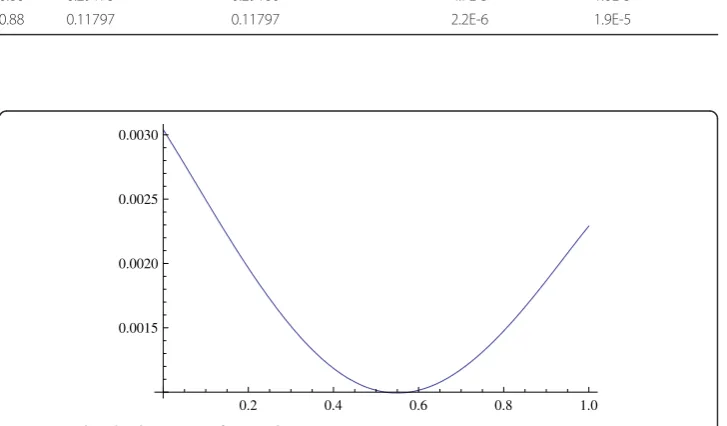
Figure 2The relative error of Example 4.2 (n= 21,N= 5).
0.2 0.4 0.6 0.8 1.0 0.00030
0.00035 0.00040 0.00045 0.00050 0.00055 0.00060
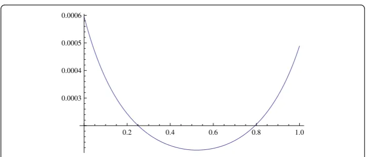
Figure 3The absolute error of Example 4.2 (n= 51,N= 5).
0.2 0.4 0.6 0.8 1.0 0.0003
0.0004 0.0005 0.0006
Contributions
Er Gao gives the main idea and proves the most of the theorems and propositions in the paper. He also takes part in the work of numerical experiment of the main results. Xinjian Zhang suggests some ideas for the prove of the main theorems. Songhe Song mainly accomplishes most part of the numerical experiments. All authors read and approved the final manuscript.
Appendix A: The reproducing kernel of H32[0, 1]
The reproducing kernel of H32[0, 1] is
K3[t,s] = 1
120+
2
2 +
3
120+
4 402+
5
120+
6
120+
7 1202
+ ⎧ ⎪ ⎨ ⎪ ⎩
1 120(s
5−5s4t+ 10s3t2),t≥s,
1 120(t
5−5t4s+ 10t3s2),t<s,
where
=a3(2b1b2+b2c1−c1c2) +a2(a3b1−a1b3+ 2a1c3−2b1c3) −2(a1+c1)(b2b3−b2c3−c2c3),
1= (c1(−2c2c3+a3c2s2−a2(−1 +s)(b3−2c3−a3s+b3s) +b2(2b3−2c3+a3(−2 +s)s))t3(10−5t+t2)),
2= (2b1b2+b2c1−c1c2−2a1b2s−2b2c1s+a1b2s2+b2c1s2) +a1c2s2+c1c2s2−a2(−1 +s)(b1−a1s+b1s))
×(2b1b2+b2c1−c1c2−2a1b2t−2b2c1t+a1b2t2+b2c1t2 +a1c2t2+c1c2t3−a2(−1 +t)(b1−a1t+b1t)),
3=c1s3(10−5s+s2)(−a2(−1 +t)(b3−2c3−a3t+b3t) −2c2c3+a3c2t2+b2(2b3−2c3+a3(−2 +t)t),
4=c1(2(c2c2(−2c3+a3s2) +a2(2b1c3−2a1c3s−a3b1s2+a1b3s2)) +b2(10b1c3+ 6c1c3+a3c1s−10a1c3s−10c1c3s−5a3b1s2 −3a3c1s2+b3(−c1+ 5a1s2+ 5c1s2)))(−2c2c3+a3cst2
−a2(−1 +t)(b3−2c3−a3t+b3t) +b2(2b3−2c3+a3(−2 +t)t)),
5= (2b1c3+ 2c1c3+a3c1s−2a1c3s−2c1c3s−a3b1s2−a3c1s2 +b3(a1s2+c1(−1 +s2)))t3(−5b2(−4 +t) +a2(10−5t+t2)),
6=s3(−5b2(−4 +s) +a2(10−5s+s2))(2b1c3+ 2c1c3+a3c1t −2a1c3t−2c1c3t−a3b1t3−a3c1t2+b3(a1t2+c1(−1 +t2))),
7= (6a22(a1s(−2c3+b3s) +b1(2c3−a3s2)) + 3a2(2c1c2(−2c3+a3s2) +b2(−b3c1+ 20b1c3+ 6c1c3+a3c1s−20a1c3s−10c1c3s−10a3b1s2
+ 10a1b3s2−3a3c1s2+ 5b3c1s2)) + 5b2(3c1c2(−2c3+a3s2)
+b2(−2b3c1+ 16b1c3+ 10c1c3+ 2a3c1s−16a1c3s−16c1c3s−8a3b1s2
Acknowledgements
The work is supported by NSF of China under Grant Numbers 10971226.
Competing interests
The authors declare that they have no competing interests.
Received: 13 January 2011 Accepted: 16 January 2012 Published: 16 January 2012
References
1. Erbe, LH, Wang, HY: On the existence of positive solutions of ordinary differential equations. Proc Am Math Soc.
120(3):743–748 (1994). doi:10.1090/S0002-9939-1994-1204373-9
2. Kaufmann, ER, Kosmatov, N: A second-order singular boundary value problem. Comput Math Appl.47, 1317–1326 (2004). doi:10.1016/S0898-1221(04)90125-3
3. Yang, F-H: Necessary and sufficient condition for the existence of positive solution to a class of singular second-order boundary value problems. Chin J Eng Math.25(2):281–287 (2008)
4. Zhang, X-G: Positive solutions of nonresonance semipositive singular Dirichlet boundary value problems. Nonlinear Anal.68, 97–108 (2008). doi:10.1016/j.na.2006.10.034
5. Ma, R-Y, Ma, H-L: Positive solutions for nonlinear discrete periodic boundary value problems. Comput Math Appl.59, 136–141 (2010). doi:10.1016/j.camwa.2009.07.071
6. Russell, RD, Shampine, LF: A collocation method for boundary value problems. Numer Math.19, 1–28 (1972). doi:10.1007/BF01395926
7. Stynes, M, O’Riordan, E: A uniformly accurate finite-element method for a singular-perturbation problem in conservative form. SIAM J Nu-mer Anal.23, 369–375 (1986). doi:10.1137/0723024
8. Xu, JC, Shann, WC: Galerkin-wavelet methods for two-point boundary value problems. Numer Math.63, 123–144 (1992). doi:10.1007/BF01385851
9. He, J-H: Variational iteration method–a kind of non-linear analytical technique: some examples. Nonlinear Mech.34, 699–708 (1999). doi:10.1016/S0020-7462(98)00048-1
10. Capizzano, SS: Spectral behavior of matrix sequences and discretized boundary value problems. Linear Algebra Appl.
337, 37–78 (2001). doi:10.1016/S0024-3795(01)00335-4
11. Ilicasu, FO, Schultz, DH: High-order finite-difference techniques for linear singular perturbation boundary value problems. Comput Math Appl.47, 391–417 (2004). doi:10.1016/S0898-1221(04)90033-8
12. Cui, MG, Geng, F-Z: A computational method for solving one-dimensional variable-coefficient Burgers equation. Appl Math Comput.188, 1389–1401 (2007). doi:10.1016/j.amc.2006.11.005
13. Cui, MG, Chen, Z: The exact solution of nonlinear age-structured population model. Nonlinear Anal Real World Appl.8, 1096–1112 (2007). doi:10.1016/j.nonrwa.2006.06.004
14. Geng, FZ: Solving singular second order three-point boundary value problems using reproducing kernel Hilbert space method. Appl Math Comput.215, 2095–2102 (2009). doi:10.1016/j.amc.2009.08.002
15. Geng, F-Z, Cui, M-G: Solving singular nonlinear second-order periodic boundary value problems in the reproducing kernel space. Appl Math Comput.192, 389–398 (2007). doi:10.1016/j.amc.2007.03.016
16. Jiang, W, Cui, M-G, Lin, Y-Z: Anti-periodic solutions for Rayleigh-type equations via the reproducing kernel Hilbert space method. Com-mun Nonlinear Sci Numer Simulat.15, 1754–1758 (2010). doi:10.1016/j.cnsns.2009.07.022
17. Zhang, XJ, Long, H: Computating reproducing kernels forW2m[a,b] (I). Math Numer Sin30(3):295–304 (2008). (in Chinese)
18. Zhang, XJ, Lu, S-R: Computating reproducing kernels forW2m[a,b] (II). Math Numer Sin30(4):361–368 (2008). (in Chinese)
19. Long, H, Zhang, X-J: Construction and calculation of reproducing kernel determined by various linear differential operators. Appl Math Comput.215, 759–766 (2009). doi:10.1016/j.amc.2009.05.063
doi:10.1186/1687-2770-2012-3
Cite this article as:Gaoet al.:Solving singular second-orderinitial/boundary value problems in reproducing
kernel Hilbert space.Boundary Value Problems20122012:3.
Submit your manuscript to a
journal and benefi t from:
7 Convenient online submission
7 Rigorous peer review
7 Immediate publication on acceptance
7 Open access: articles freely available online
7 High visibility within the fi eld
7 Retaining the copyright to your article