ISSN: 2146-4138 www.econjournals.com
Poverty, Growth and Inequality in Developing Countries
Housseima Guiga
Faculty of Economic Sciences and Management of Tunis, Tunis El Manar University, TUNISIA.
Email: [email protected]
Jaleleddine Ben Rejeb
Higher Institute of Management of Sousse, University of Sousse, TUNISIA.
Email: [email protected]
ABSTRACT: The purpose of this paper is to assess the position of some developing countries in relation to different theories about the relationship between poverty, growth and inequality. We conducted an econometric analysis through a study using panel data from 52 developing countries over the period 1990-2005, to determine the main sources of poverty reduction and show the interdependence between poverty, inequality and growth by using a system of simultaneous equations. This method is rarely applied econometric panel data and especially in the case studies on poverty. Our results indicate that the state investment in social sectors such as education and health and improving the living conditions of the rural population can promote economic growth and reducing inequality. Therefore, the Kuznets hypothesis is based on a relationship between economic growths to income inequality is most appropriate.
Keywords: Poverty, Growth; Inequality; Panel Data; Simultaneous System Equations. JEL Classifications: C30; C33; I32; O15
1. Introduction
Poverty is a global phenomenon which is increases day by day. This phenomenon is related to areas such as Sub-Saharan Africa, Asia and Latin America. Similarly, poverty affects several million people in Europe. Among the 400 million people of the European Union member countries, 60 million live below the poverty line (set at 50% of median income in each country), and 2.7 million people are homeless. For an international poverty line at $ 1.08 per day, 75% of the poor in the developing world are concentrated in rural areas, while only 58% of its population is rural.
Several years ago, the fight against poverty has become a constitutive element of development policy. A set of countries in the international community has been devoted entirely to the fight against poverty in its monetary dimension, educational and equity. Their main objective "Millennium Development Goal" is based on the reduction by half between 1990 and 2015 the proportion of people whose income is less than one dollar per day.
Since the publication of the annual report of the Global Report of Human Development (1990), most international aid agencies and development donors, have reserved their efforts to economic growth seen as a fundamental factor in the process of fight against poverty.
They consider that economic growth is favorable to reduce poverty. This idea is based on theoretical and empirical evidences. For example, Ravallion and Chen (1996) showed, from an econometric model, that the elasticity of poverty to economic growth is always negative for different poverty lines.
However, the results are not similar for all geographical areas. As it is noted in the World Development Report, the countries of East Asia, especially China accounted for most of the world’s decline in extreme poverty since 1980, while the sub- Saharan Africa has succeeded in reducing poverty only in 1990 and 2004 despite the economic policies adopted.
It is undeniable that the underdeveloped world has marked economic progress especially during the last two decades. Hence the question arises: Why the living conditions of the poor do not follow the overall improvement observed in the world in general and in the Third World in particular?
Kakwani and Pernia (2000), for example, consider that growth is pro-poor if it is accompanied by a reduction in inequality.
Bourguignon (2003) showed that the trends in poverty are not systematically related to economic growth because they can also be associated with inequality in the economy. This explanation relies on a mechanical relationship between growth, inequality and poverty.
In fact, Bourguignon (2003) expressed the changes in poverty as the sum of changes in the average level of income and changes in the level of inequality.
The problem we try to solve here is to identify the factors that most influence the evolution of poverty and clarify by what mechanism is the transmission of economic growth and income inequality into poverty. To achieve this goal, we are led to resort to panel data from 52 developing countries over the period 1990-2005.
2. Economic Growth as a Tool for Reducing Poverty
Many economists such as Adam Smith, Karl Marx, John Stuart Mile, considered the capital accumulation and enrichment as a mean of eradicating extreme poverty and shortage.
Economic growth creates employment because it requires a workforce. According to data of the Global Report of Human Development (2003), many countries have found difficult to combat monetary poverty, due to the lack of economic growth during the 90s decade and that regions with faster economic growth (countries of East Asia and countries of South Asia, with respective growth rates of 6.4% and 3.3%) reduced, a more important monetary poverty.
For example, between 1987 and 1998, growing fast, the proportion of poor decreases by 16.7 points in the low-income countries and 18.3 points in the middle-income countries.
Based on average expenditures derived from household surveys, Ravallion and Chen (1996, p.34) regressed the elasticity of poverty incidence for consumption on different Poverty lines.
The estimation results show that the elasticity of poverty to growth is still negative, it varies between -0.53 and -3 12 for different poverty lines. Thus, if growth would increase by 1 percentage point, the share of population living on less than $ 1 per day, would be reduced by 3.1 percentage points.
Barro (1997), to answer the question of whether economic growth reduces poverty, made a regression of 30 countries, the rate of income growth leading to respective first and second poorest quintiles the rate of growth GDP per capita in PPP.
The results show that the elasticity of GDP per capita growth with income growth of 20% poorest is equal to 0.921 and the 40% poorest follows closely the growth of income per head.
The article of Dollar and Kraay (2000) « Growth is good for the poor » contribute to reaffirm the importance of economic growth policies to reduce poverty. They divide the sample between periods of crisis and periods of expansion.
The results show the existence of a very close correlation between the incomes of poor and average income: the correlation coefficient is 1.08 for the period of crisis and 1.09 for the periods of normal growth. Contrary to conventional ideas, Dollar and Kraay (2000) show that in times of crisis or downturn, the income of the poor do not fall more than income per head and there is no evidence that crises affect income of the poor in a manner disproportionate.
Similarly, they show that the effect of growth on incomes of the poor is even in poor countries than in rich countries and the growth caused by the policies of the state, is more beneficial to the poor than the economy in general.
Alesina and Rodrik (1994) demonstrate using data from over 40 countries that inequality, particularly in access to land and income, is detrimental to the growth itself and its effects on reducing poverty.
The empirical record shows that poverty is intimately linked to economic growth. This economic growth is related to the level of inequality and the nature of distribution which is equal or unequal.
In the next section we will mention the different theoretical and empirical findings addressing the relationship between growth and inequality. Inequality: the element that minimizes the role of economic growth in the process of poverty reduction
The first theoretical foundation that focuses on the relationship between growth and inequality is the Kuznets hypothesis (1955) based on a curvilinear relationship between growth and income inequality.
This inverted U-curve can be decomposed into three phases. In the early stages of development, characterized by very low income levels, investment in infrastructure capital and natural capital is the main mechanism of growth, inequality encourages growth by sharing resources for those who save and invest more. Moreover, as the population becomes urbanized and industries grow, inequality rises
In a more advanced stage of development, as wealth accumulates, the transition from physical investment to investing in technology and human capital has reduced inequality.
The third phase is characterized by a greater level of wealth. The increase in human capital takes the place of physical capital accumulation as the main source of growth. The inequality is slowing while growth continues to be realized.
This inverted U curve shows the idea that the process of economic development reflects a transition from an agricultural economy with low productivity to an industrial economy with high productivity. Kuznets explains this principle by the hypothesis of dualism which he considers two agricultural and non agricultural (very unequal). According to this hypothesis, the evolution of inequality during this period is attributed to the reduced share of the agricultural sector in the economy and its replacement by the industrial sector.
A study of the Kuznets hypothesis developed by Deininger and Squire (1996) conducted on panel data shows the absence of a significant relationship between inequality and growth which led the authors to study the relationship of reverse causality, ranging from inequality to growth.
The first two are from Alesina and Rodrik (1994) and Persson and Tabellini (1994), according to them where inequalities are too high induce a demand for redistribution and a high level of taxation that discourages investment in human and physical capital which is detrimental to growth.
Deininger and Squire (1998) conducted a cross-sectional regression of 44 countries for the years 1960 and 1992 to clarify the impact of inequality in land distribution and income growth.
The estimation results show that an increase of one standard deviation of 0.4 points in the Gini coefficient causes a decrease in average growth rate per capita of 0.4 percentage points. However, the coefficient of inequality becomes non significant by introducing dummies regions. While the Gini coefficient of land distribution is still significant even if the regional dummies are introduced.
This leads us to conclude that a better measure of disparity is the Gini of the earth. Thus, the evolution of poverty must be decomposed into effects related to growth and the other resulting in inequality.
Bourguignon (2003) has reported that growth modifies the distribution of income, which itself partly determines the growth, nature, level and its impact on poverty. Similarly, he stressed on the idea of maintaining the redistribution as a complementary element of growth to achieve a remarkable reduction in the level of poverty in the short and long term.
Ravallion (2001) shows that the reduction of inequality results in a faster pace of poverty reduction. He has proved, on the basis of an econometric study, that countries having higher average income per head, registering a reduction of poverty from 1.3% to a high level of inequality, while the reduction is 10% to a low level of inequality
3. Modeling the Interaction between Poverty, Growth and Inequality
We will try in this part using econometric models involving poverty in relation to growth and inequality and other explanatory factors. For this, we use an econometric panel data by taking a sample of 52 developing countries over a period displaying from 1990 to 2005.
3.1. Specification of models and variables description Model 1:
The first model expresses poverty in terms of two principal variables which are economic growth and inequality of income and other explanatory factors. Panel data regression model is shown bellow in the simplest way (Meng et al., 2005):
Log(P)it = αi + α1log(GDP)it+ α2log(Gini)it+ α3log(infl)it +α4log(saving)it +α5log(school)it+ εit (1)
With Pit: is the poverty head-count index in terms of income. It is the proportion of people below the
poverty line (named poverty rate).
GDPit: is the real gross domestic product per capita based on purchasing power parity. GDP per head
can take into account the impact of growth on poverty.
Giniit: is the Gini coefficient which measured in term of income.
Inflit: is the rate of inflation, which captures the impact of macroeconomic stability on poverty. Savingit: is the rate of investment as a percentage of GDP.
Schoolit: is the secondary enrollment rate reference to human capital. αi is the effect of specific countries and εit is the error term.
To estimate this equation it is necessary to execute the Hausman tests comparing the estimator "within" and the least squares estimator quasi-generalized. This test leads to reject the exogeneity of the individual effect.
The OLS estimator for the first differences (FD OLS) removes individual fixed effect. The estimation of this linear model is done by the method of generalized least squares because the Hausman test allows us to choose a random effects model.
Model 2:
Concerning the second model, we proceed to estimate the growth equation that will allow us to firstly, identify the factors contributing to the promotion of growth and secondly, to identify the impact of inequality on economic growth. The dynamic panel model that will be used based on Forbes (2000) is as follows:
1i,t i 1 1 , 1 2 2 , 1 3 3 , 1 4 4 , 1 5 5 , 1 6 6 , 1
x
(2)
it i t i t i t i t i t i t it
y
x
x
x
x
x
x
U
Where γi is the individual effect and Uit is the error term.
yitis the average annual growth rate of GNP per capita.
x1i, t-1 is the GNP per capita calculated in $ (U.S. List Price).
x2i, t-1 is the Gini index with the expected sign of the coefficient is positive.
x3i, t-1 is the secondary enrollment rate.
x4i, t-1 is the infant mortality rate (per 1,000 children) for children aged 5 and under.
x5i, t-1 is the percentage of gross domestic savings (share in GDP).
x6i, t-1 is the weight of the rural population in total population.
This dynamic panel model includes a lagged dependent variable that is correlated with the error term (E (yi, t-1Uit) ≠ 0) which makes the estimation of intra-individual ordinary least squares (OLS) biased and non-convergent.
Similarly, the explanatory variables are correlated with individual effects E (xit αi-1) ≠ 0.
Arellano and Bond (1991) suggest a technique for estimating the moments’ generalized method which not only corrects the bias introduced by the lagged endogenous variable, but also allows the correction of measurement error in the other regressors. The principle of this method is to consider the model in first differences:
, 1
(
)
(3)
it i t it ity
y
x
u
In fact, the method of MMG is to take for each period the first difference equation to eliminate the effects of specific countries (αi), and then instrument the first differences of variables in the
• The test of Sargan (1958) of suridentifiantes restrictions: it is a necessary condition that the estimated equation should be suridentifiant view that the number of orthogonality conditions corresponding to the hypotheses (the number of instruments) should be higher than the number of parameters to estimate.
The test statistic follows the chi-square law of order q (q = number of external instruments - number of explanatory variables).
• The test of autocorrelation of second order in which the error terms should not be correlated in series: E (uit ui,t-s) = 0 pour tout s ≥ 1. → E (∆uit , ∆ui,t-2 ) = 0
This is a test of second order between the first differences of individual error terms and time. However, this equation suffers from a problem of endogeneity. In fact, referring to theoretical work, the Kuznets hypothesis (1955) focuses on a causal relationship conversely, from growth to inequality and which is written as follows:
0 1 2 3 , 2
log(
Gini
it)
log(
Pnb
it)
log(
Invst
it)
log(
Infl
it)
i t (4)Whose dependent variable Giniit: is the Gini coefficient and variable independent are
Pnbit: Gross National Product per capita
Invstit: the rate of gross investment as a percentage of GDP.
Inflit: the rate of inflation is the annual percentage change in prices acquiring a fixed basket of goods
and services.
To clarify this interaction, we try to analyze simultaneously the interdependence between poverty, inequality and growth using a system of simultaneous equations which is written as follow:
Model 3:
0 1 2 , 1t
0 1 2 3 , 2
0 1 2 3 4 5
log(
)=
log(
)
log(
)
log(
)
log(
)
log(
)
log(
)
log(
)
log(
)
log(
)
log(
)
log(
)
log(
it it it i
it it it it i t
it it it it it
Pauvreté
Pnb
Gini
Gini
Pnb
Invst
Infl
Crois
Pnb
Gini
Txscho
Sante
Rural
it)
6log(
Ep
arg
ne
it)
i, 3t
This system of equations includes three models defined above with the first model is inspired by the work of Meng et al., (2005) and expresses the rate of poverty (Pit) based on GNP per capita (Pnbit) and
the Gini coefficient (Giniit). The second model represents the equation of inequality (Kuznets, 1955)
and the third is the function of economic growth. 3.2. The Results of Estimations
It is necessary to appeal to a bivariate analysis to test the possible presence of a problem of multicollinearity between the explanatory variables.
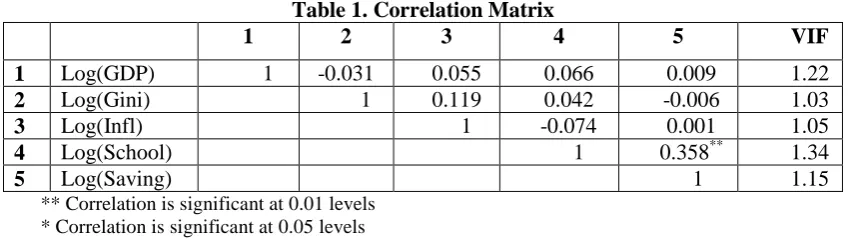
Table 1. Correlation Matrix
1 2 3 4 5 VIF
1 Log(GDP) 1 -0.031 0.055 0.066 0.009 1.22
2 Log(Gini) 1 0.119 0.042 -0.006 1.03
3 Log(Infl) 1 -0.074 0.001 1.05
4 Log(School) 1 0.358** 1.34
5 Log(Saving) 1 1.15
** Correlation is significant at 0.01 levels * Correlation is significant at 0.05 levels
The correlation matrix presented in Table 1, shows that the explanatory variables are weakly correlated in general. But the correlation between enrollment and investment rates is statistically significant at the 1% and by conducting the test of FIV1, there is an absence of multicollinearity.
In fact, the linear independence implies a VIF equal to 1 and VIF collinearity implies a VIF greater than 10. In our case, the variables are much lower than 10 (Neter et al., 1985), the problem of multicollinearity does not seem critical.
1 The Variance Inflation Factor measures the degree to which the variance of coefficients in a partial regression
Thus, for the equations considered, Hausman tests comparing the estimator "within" and the least squares estimator quasi-generalized leads to systematically reject the exogeneity of the individual effect. The various regressions are shown in Table 2.
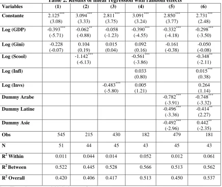
Table 2. Results of linear regression with random effects
Note: The endogenous variable is the rate of poverty
*, **, *** Indicate statistical significance respectively at 10%, 5% and 1%.
The first estimate of the model shows that an increase in income per head is pro-poor. In fact, the elasticity of poverty rate in GDP per capita is negative and significant at the 1% (column 1 of Table 2) and an increase in GDP per capita of 1% will lead to a decrease in the poverty rate of 40%. This was consistent with results obtained by Ravallion and Chen (1996) and Dollar and Kraay (2000), under which economic growth plays a key role in reducing poverty.
Concerning the logarithm of the Gini coefficient (column 1), it is negative and insignificant. Regarding the control variables, the results show that an increase in secondary enrollment reduces poverty and an increase of 1 percentage point of enrollment would lead to a decrease in the poverty rate of 1.14 percentage points. Similarly for the coefficient of the logarithm of the rate of investment, it is negative and statistically significant at 1% and a 1% increase in the investment rate would reduce the poverty rate of 48% (column 3).
It should be noted that the rate of inflation has no significant impact and that the results did not differ in a major way by introducing the dummy variables. The values in the intercept being 2.85 for Africa, 2.07 (2.85-0.782) for Arabic, 2.36 (= 2.85-0.49) for Latin America and Asia. We concluded that there is not a very important effect of regions. That is why the explanatory power (R2 overall) does not improve by introducing dummy variables.
Table 3 introduces the estimation of second model using the fixed effect (column 1), the random effect (column 2) and the technique of Arellano and Bond GMM (column 3). The model was chosen as logarithmic.
Variables (1) (2) (3) (4) (5) (6)
Constante 2.125***
(3.08) 3.094*** (3.33) 2.811*** (3.75) 3.091*** (3.24) 2.850*** (3.77) 2.731*** (2.48)
Log (GDP) -0.393***
(-5.71) -0.062** (-0.88) -0.058 (-1.23) -0.390*** (-4.55) -0.332*** (-4.18) -0.298*** (-3.50)
Log (Gini) -0.228
(-0.07) 0.104 (0.19) 0.015 (0.04) 0.092 (0.16) -0.161 (-0.38) -0.050 (-0.08)
Log (Scool) -1.142***
(-6.13)
-0.561*** (-3.86)
-0.348** (-2.11)
Log (Infl) 0.033
(0.80)
0.015*** (0.38)
Log (Invs) -0.483***
(-5.80)
0.005 (1.21)
0.264 (1.14)
Dummy Arabe -0.782***
(-3.91)
-0.748*** (-3.32)
Dummy Latine -0.496***
(-3.36)
-0.414** (2.27)
Dummy Asie -0.492***
(-2.96)
0.442** (-2.35)
Obs 545 215 430 182 479 181
N 51 44 45 43 45 43
R2 Within 0.011 0.044 0.014 0.052 0.012 0.061
R2 Between 0.522 0.445 0.528 0.566 0.513 0.562
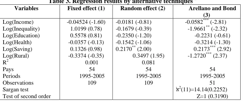
Table 3. Regression results by alternative techniques 2
Variables Fixed effect (1) Random effect (2) Arellano and Bond
(3)
Log(Income) Log(Inequality) Log(Education) Log(Health) Log(Saving) Log(Rural) R2
Pays Periods Observations Sargan test
Test of second order
-0.04524 (-1.60) 1.0199 (0.78) 0.5578 (0.81) -0.0357 (-0.13)
0.1326 (0.98) -0.3374 (-0.35)
0.001 54 1995-2005
109
-0.0181 (-0.81) -0.1679 (-0.39) -0.2350 (-1.20) -0.1542 (-1.06) 0.2170** (2.00)
0.3497 (1.95) 0.081
54 1995-2005
109
-0.0582*** (-2.81) -1.9661** (-2.32) -0.2231 (-0.61) -0.3214 (-1.30) 0.2173*** (2.92) -1.2720*** (2.37)
54 1995-2005
51 ﭏ2(11)=14.14(0.2252)
Z=1 (0.3190)
From this table, we see that whatever the estimation method (fixed effect or random effect), the model used is not efficient. Indeed, the explanatory power is very low (R2 overall). Similarly, no weighting of variables is significant, with the exception of coefficient on variable savings (significant at seuil5%).
In our regressions, as mentioned previously, the two methods are not efficient because of the presence of delayed income. So we opted for the GMM method of Arellano and Bond (1991) in two steps that we can correct this problem.
Prior to the estimation of the GMM dynamic model, we must ensure the validity of lagged variables as instruments. The Sargan test statistic equals ﭏ2 (11) = 14.14 4 with a probability greater than 5%, which allows us to accept the null hypothesis that our equation is suridentifiant.
Concerning the residual autocorrelation test of second order, the probability of accepting the null hypothesis (H0: no autocorrelation) is equal to 0.319 which allows us to deduce that the errors are not correlated.
The model results show the growing significance of several variables of interest.
The coefficient
of income is negative and highly significant at 1%. An increase of 1 percentage point to gross
national income per head leads to a decrease in the rate of growth of GDP of 1.05 percentage
points (the coefficient of this variable is equal to -1.0582).
According to Arjona et al., (2002, p.23), this negative effect of initial income on the annual growth rate is explained by Solow and Swan (1965), as absolute convergence of economies which means a level of capital per head identical for all countries
For the variable inequality, the coefficient is negative and significant at 5% and for an increase of 1 percentage point of inequality there is a decrease of the growth rate of GDP of 1.96 percentage points.
The coefficient on the percentage of rural population is negative and significant at 5% and for an increase of 1 percentage point of the rural population there is a decrease of the annual growth rate of GDP of 1.27 percentage points.
The ratio of gross domestic savings is positive and highly significant and for an increase in gross domestic saving of 1 percentage point we have an increase is the growth rate of GDP of 0.21 percentage point.
Finally, it should be noted that the coefficients associated with education and health are not significant. Referring to these two models and that of the Kuznets curve, we see the interdependence between poverty, growth and inequality. Therefore, we will jointly estimate the three models in the form of a system of simultaneous equations.
To identify the possible presence of endogeneity problem, we make use of the test Durbin-Wu-Hausman, which is in two stages. Initially, we proceed to the regression of each endogenous variable on all exogenous variables (Davidson and MacKinnon, 1993). Then, we recover the residues of the first regression and included them in the initial model.
2 The dependent variable is the average annual growth rate of GNP per capita and the figures in brackets are
In our case, we will test the endogeneity of the variable GNP per capita and the Gini. The test results of Durbin-Wu-Haussman show that the residues of the original equation are significant and thus there is a problem of endogeniety.
On the other hand, it is necessary to check two conditions identification: the conditions of order and the rank conditions. The rank condition is a necessary and sufficient condition for identification, but in practice it is difficult and sometimes impossible to implement. That's why researchers are content most often order a condition that is determined equation by equation.
To implement this test, we proceed as follows: Where:
g: the number of endogenous variables of the model (or the number of equations); g': the number of endogenous variables included in an equation;
K: the number of exogenous variables of the model;
K ': the number of exogenous variables contained in an equation.
Our model has three equations, g = 3 (which are the Headcount, GDP and GINI), K = 7 (6 exogenous variables and the constant).
First equation: g’= 2 and K’= 1. That is to say: g – 1<g-g’+K-K’: the equation is therefore over-identified.
Second equation: g’=1 and K’=2. That is to say: g – 1<g-g’+K-K’: the equation is therefore over-identified.
Third equation: g’=2 and K’=5. That is to say:g – 1<g-g’+K-K’: the equation is over-identified. In conclusion, the identification condition is satisfied and the model is over-identified and can be estimated.
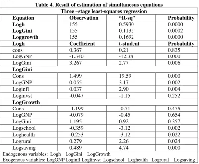
Table 4. Result of estimation of simultaneous equations Three –stage least-squares regression
Equation Observation “R-sq” Probability
Logh LogGini Loggrowth
155 155 155
0.5930 0.1135 0.1692
0.0000 0.0002 0.0000
Logh Coefficient t-student Probability
cons 0.367 0.21 0.835
LogGNP -1.340 -12.38 0.000
LogGini 3.267 2.77 0.006
LogGini
Cons 1.499 19.59 0.000
LogGNP 0.055 3.17 0.002
Loginfl 0.037 2.90 0.004
Loginvst -0.047 -1.15 0.252
LogGrowth
Cons -1.199 -0.71 0.475
LogGNP -0.079 -0.45 0.654
LogGini 1.195 0.92 0.357
Logschool -0.359 -3.12 0.002
Loghealth -0.253 -3.12 0.022
Logrural 0.279 2.26 0.024
Logsaving 0.489 4.74 0.000
Endogenous variables: Logh LogGini LogGrowth
Exogenous variables: LogGNP Loginfl Loglinvst Logschool Loghealth Logrural Logsaving
While the increase of 1 percentage point of the Gini coefficient would result in an increase of 3.26 percentage points in the poverty rate.
The last variable (Gini index) is itself determined by the GNP per capita and the inflation rate which are significant at 1%. In fact, the increase of 1 percentage point of GNP per capita would generate increased levels of inequality averaged of 0.05 percentage points and an increase by 1 percentage point of inflation is equivalent to an increase the level of inequality of 0.03 percentage points.
This result is expected because the poor are less protected against inflation as the wealthiest in society. Thus, inflation aggravates the situation of the poor which will lead to a higher gap between rich and poor in society.
It should be noted that the rate coefficient of investment is not significant. Concerning the reverse causality, from inequality to growth, we do not see a significant impact of the Gini coefficient on the rate of economic growth. We conclude that the hypothesis of Kuznets (1955), ranging from growth to inequality, is the most appropriate. This does not preclude having others factors which have a significant impact on economic growth.
The results show a positive impact on the percentage of rural population and gross domestic savings rate of growth. These last two are significant respectively at the 5% and 1%. Indeed, the increase of 1 percentage point of the rural population generates an increase in the rate of growth of output per head of 0.27% and the increase of 1 percentage point from gross domestic savings is equivalent to an increase economic growth rate of 0.48%.
Similarly, the results indicate that the coefficient of infant mortality rate is negative and significant at 5%. This implies an increase of 1 percentage point of infant mortality rates imply a reduction in the rate of economic growth of 0.25 percentage points. Thus, it is essential to the state to improve health services sector which is in favor of the economic growth. It should be noted that coefficient of secondary school enrollment rate is significant at 1% but does not admit the predicted sign (positive).
4. Conclusion
The general topic of this article has focused on the phenomenon of poverty. The main objective of this study is to assess the factors that most influence the evolution of poverty and determine the nature of interaction between poverty, growth and inequality.
Some authors, such as Dollar and Kraay (2000) find that the role of economic growth is crucial for poverty reduction and economic growth plays a direct role in increasing the incomes of the poor. Indeed, several speakers in the field of development focus on accelerating growth to achieve the international development goal, which is to reduce by half the proportion of poor in the world between 1990 and 2015.
However, growth is not sufficient for poverty reduction; it is necessary but it must be also accompanied by the introduction of policies to reduce inequalities. In fact, for a rate of economic growth, poverty is not declining at the same pace in all countries or all times. This amount to the extent of the reduction of poverty depends on change in the distribution of income growth. In addition, it is depends on the initial inequalities in terms of income, assets and access to opportunities that allow poor people to enjoy the fruits of growth.
Bourguignon (2003) showed that a high level of inequality is associated with a slower reduction in poverty during episodes of positive growth. He stressed that maintaining the redistribution as a complementary element of growth to achieve a lower level of poverty in the long term.
In this article, to understand the mechanism of poverty reduction, we estimate the relationship between poverty, inequality and growth and other control variables by conducting regressions performed on panel data from 45 developing countries during the period 1990-2005.
The main observations that can be drawn from the regressions are as follows:
The increase in per capita income reduces the poverty rate. The results show that an increase of 1 percentage point of GDP per capita causes a reduction of poverty rate of 0.40 percentage points. Thus, economic growth plays a key role in reducing poverty.
We showed that there is not a significant impact of Gini coefficient on the economic growth and thus the Kuznets hypothesis, ranging from growth to inequality, is the most appropriate. Concerning other socioeconomic factors, they play an important role in promoting economic growth that is reducing poverty.
The estimation shows that the increase in percentage of rural population generates an increase in economic growth, which implies that the population of developing countries lives in rural areas, and is active in agriculture sector. Similarly, gross domestic savings has a positive impact on economic growth. While infant mortality rate, induces a decrease in the rate of economic growth which encourages the state to improve services in the health sector.
Thus, it is essential to apply appropriate social policies including the establishment of institutions, education and skill’s development and the improvement of health services, especially in the fight against infectious diseases. Also, it is necessary to give more interest to rural areas for one hand, reduce inequalities between rural and urban areas and secondly, to accelerate the pace of economic growth.
References
Alesina, A., Rodrik, D. (1994), Distributive Politics and Economic Growth, Quarterly Journal of Economics, 109(2), 465-490.
Arellano, M., Bond, S. (1991), Some tests of specification for panel data: Monte Carlo evidence and an application to employment equations. The Review of Economic Studies, 58, 277–297.
Arjona, R., Ladaique, M., Pearson, M. (2002), Social Protection and Growth, OECD Economic Review, 35(2), 7-45.
Barro, R.J. (1997), Determinants of Economic Growth: A Cross-Country Empirical Study, Cambridge, MA,
Bourguignon, F. (2003), The poverty-Growth-Inequality Triangle, Contribution presented in Indian Council for Research on International Economic Relations, in New Delhi, India.
Davidson R., MacKinnon J.G., (1993), Estimation and Inference in Econometrics, Oxford University Press, New York.
Deininger, K., Squire, L. (1996), A new data set measuring income inequality, The World Bank Economic Review, 10(3), 565-592.
Deininger, K., Squire, L. (1998), New ways of looking at old issues: inequality and growth, Journal of Development Economics, 57(2), 259-287.
Dollar, D., Kraay, A. (2000), Growth is Good for the Poor, Development Research Group, World Bank.
Forbes. K.J. (2000), A Reassessment of the Relationship between Inequality and Growth, American Economic Review, 90(4), 869-887.
Global Report of Human Development (1990), Paris, Economica. Global Report of Human Development (2003), Paris, Economica.
Kakwani, N., Pernia, E. (2000), What is Pro-Poor Growth? Asian Development Review, 18(1), 1-16. Kraay, A. (2006), When is Growth Pro-Poor? Evidence from a Panel of Countries, Journal of
Development Economics, 80(1), 198-227.
Kuznets, S. (1955), Economic Growth and Income Inequality, American economic Review, 45(1), 1-28.
Meng, X., Gregory, R., Wang, Y. (2005), Poverty, Inequality and Growth in Urban China, 1985-2000, Journal of Comparative Economics, 33(4), 710-729.
Neter, J., Wasserman, W., and Kutner, M.H. (1985), Applied linear statistical models (2nd ed.). Homewood, IL: Richard D. Irwin, Inc.
Persson, T., Tabellini, G. (1994), Is Inequality Harmful for Growth? American Economic Review, 84(3), 600-621.
Ravallion, M., Chen, S. (1996), What can new survey data tell us about recent changes in distribution and poverty? The World Bank Economic Review, 11(1), 345-361.
Ravallion, M. (2001), Growth, Inequality and Poverty: Looking Beyond Averages. World Development, 29, 1803-1815.