ISSN: 2008-6822 (electronic)
http://dx.doi.org/10.22075/IJNAA.2020.4217
An Analysis of A Fishing Model with Nonlinear
Harvesting Function
E. SOROURIa, M. ESHAGHI GORDJIa,∗, R. MEMARBASHIa
aDepartment of Mathematics, Semnan University,
P. O. Box 35195-363, Semnan, Iran.
(Communicated by Javad Damirchi)
Abstract
In this study, considering the importance of how to exploit renewable natural resources, we analyze a fishing model with nonlinear harvesting function in which the players at the equilibrium point do a static game with complete information that, according to the calculations, will cause a waste of energy for both players and so the selection of cooperative strategies along with the agreement between the players is the result of this research.
Keywords: natural resource management, game theory, bioeconomic models, nonlinear dynamical systems, fishery, harvest function.
2010 MSC: 91B76; 91A80.
1. Introduction
Since game theory examines situations in which decision-makers interact, this theory has many applications in the commercial competition between individuals, companies, and countries (see [2],[8],[9],[14] and [15]).
For example, using this theory, we can examine how to use renewable natural resources and different strategies. Consider a river, lake or sea exploited by fishermen or companies. If the number of fishermen is increased or more fish are harvested, it will lead to the extinction of the generation of fishes in that source.
If fishering from the source is done only by a fisherman, he(or she) will consider the amount of current harvest because he(or she) knows that the amount of fish may be reduced and harvesting in
∗Corresponding author
Email addresses: [email protected](E. SOROURI ), [email protected](M. ESHAGHI GORDJI ), [email protected](R. MEMARBASHI )
prevent the extinction of species (see [1],[3],[4],[11],[12],[13] and [18]).
Of course, a large number of these studies have been investigated in Dynamic Systems (see [5], [6], [10], [16], [17] and [19]).
The logistic equation with density-dependent harvesting (see [7]) is
dN
dt =rN(1− N
K)−H(t).
whereN is the population biomass of fish at timet,ris the intrinsic rate of growth of the population,
K is the carrying capacity, andH(t) as the harvest function is
H(t) =qEN(t)
whereE is the fishing effort, the intensity of the human activities to extract the fish andq ≥0 is the catchability coefficient which is defined as the fraction of the population fished by a unit of effort. In the above fishing mdel and many other models, the harvest function is linear in terms ofN(t) but we want to examine the effect of the nonlinear harvest function of H(t) =qE(N(t))2 and since that
fishermen or companies usually harvest individually and based on their own profits, at the point of equilibrium of the system we consider a static game with complete information and as a result we calculate the amount of the waste of effort and energy.
2. Main results
In this model, we consider the relation between net growth, W, and the carrying capacity, K, a logistic growth function. So, we have
W =rN(1− N
K). (2.1)
Assuming a nonlinear harvest function, H =qEN2, the dynamics of this model is
dN
dt =rN(1− N
K)−qEN 2
.
It can be written as follows
dN
dt =rN(1− N K0
)
where K0 = r+rKqEK. This system has a trivial equilibrium, N = 0, and an non-trivial equilibrium, N =K0 = r+rKqEK.
Considering f(N) = rN(1− NK)−qEN2, we have dN
dt = f(N). Since
df(N)
dN = r−2
rN
K −2qEN,
then df(0)
dN = r > 0 so the trivial equilibrium point is unstable, and at the non-trivial equilibrium df(K0)
dN =
−r2−qEK
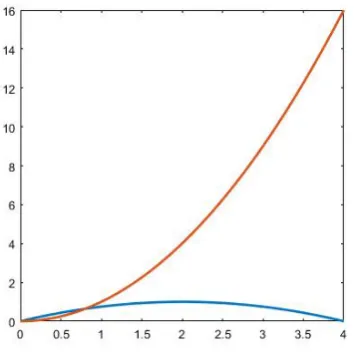
Figure 1: The functinsW =rN(1− NK), H =qEN2 in whichr = 1, q= 1, E = 1 and K = 4.
On the other hand the differential equation of this system is a separable type and it is solved by a method called separation of variables.
By solving this equation and taking B = |K0N−(0)N(0)|, it follows that if K0 −N > 0 then N(t) =
BK0ert
1+Bert is the solution of this differential equation and since limt→+∞N(t) = K0, it implies that
the non-trivial equilibrium is asymptotically stable and if K0−N < 0 then N(t) = −BK0e
rt
1−Bert is the
solution of the differential equation and limt→+∞N(t) = K0 implies that the non-trivial equilibrium
is asymptotically stable.
According to the above, when the system reaches the equilibrium point, where H = W (see Figure 1), we have
N = rK
r+qEK. (2.2)
Which shows the relation between the equilibrium mass and the effort. By substituting (2.2) in
H(t), the relation between the level of effort and the harvest is
H =qE( rK (r+qEK))
2. (2.3)
We assume that there are two fishing companies,A1 and A2, which use this source separately. They
as players do a static game with complete information in devoting the amount of effort to harvest. If E1 and E2 respectively represent the level of effort of players A1 and A2 then the total effort to
harvest from this source isET =E1+E2 and the total harvest of this effort isHT =qET((r+qErKTK))2.
In this model, we assume that the share of each company (player) is equal to its share of total effort in other words
H1 = E1 ET
HT =
E1 ET
qET(
rK
(r+qETK)
)2 =qE1(
rK
(r+q(E1+E2)K))
2,
H2 = E2
ET
HT =
E2 ET
qET(
rK
(r+qETK)
)2 =qE2( rK
(r+q(E1+E2)K)
)2
where HT =H1 +H2.
(r+q(E1+E2)K)2
To find the Nash equilibrium we use the best response method. In this way, we first do the calculations for player 1. So, assuming that E2 =E2 is positive and constant, we have
UA1(E1, E2) = 0 =⇒E1 = 0∨E1 =
√
P r2 qC −β.
where β= (qKr +E2). But
E1 =
√
P r2
qC −β >0⇐⇒E2 < r(
√
P qC −
1
qK). (2.4)
On the other hand, if ∂UA1(E1, E2)
∂E1
= qr2P K2(r+q(E1+E2)K)−2r2q2P K3E1
(r+q(E1+E2)K)3 − c = 0 then by a simple
calculations we have
E13+ 3E12β+ (3β2 +r
2P
qC )E1 = r2P
qC β−β
3 (2.5)
where β= (qKr +E2).
We considerf1(E1) = E13+ 3E12β+ (3β2+
r2P
qC )E1 andf2(E1) = r2P
qC β−β
3 that according to (2.4)
and β = qKr +E2 >0 always f2(E1) = r
2P
qC β−β
3 >0.
On the other hand, limE1→+∞f1(E1) = +∞and limE1→−∞f1(E1) =−∞and alsof1(E1) =E1(E12+
3βE1 + (3β2+ r
2P
qC )) thatE
2
1 + 3βE1+ (3β2 +r
2P
qC ) has ∆ =−3β
2−4r2P
qC <0 thenf1(E1) only has
a real root E1 = 0.
Since df1(E1)
dE1
= 3E12+ 6βE1+ (3β2+ rqC2P) then f1(E1) forE1 >0 is always an increasing function. According to the above, functionsf1 and f2 forE1 >0 intersect each other exactly at one point then UA1(E1, E2) for 0< E2 < r(
√ P qC −
1
qK) has exactly a local extremum that we show it withE1◦.
In order to determine the type of this extremum, we use the first derivative test for UA1(E1, E2)
in the neighborhood of this point,E1◦. Since E1◦ >0 , we consider ϵ >0 such thatE1◦−ϵ >0 in this case
dUA1(E1◦,E2)
dE1 =
−C(qKE1◦+(r+qKE2))3−q2r2P K3E1◦+qr2P K2(r+qKE2)
(qKE1◦+(r+qKE2))3 = 0, dUA1(E1◦+ϵ,E2)
dE1 =
−C(qK(E1◦+ϵ)+(r+qKE2))3−q2r2P K3(E◦
1+ϵ)+qr2P K2(r+qKE2)
(qK(E◦1+ϵ)+(r+qKE2))3
= −Cq3K3ϵ3−3qKCθ1ϵ−3q2K2Cθ1ϵ2−q2r2K3P ϵ
(qK(E◦1+ϵ)+(r+qKE2))3 <0
where θ1 =qKE1◦+ (r+qKE2)>0,
dUA1(E1◦−ϵ,E2)
dE1 =
Cq3K3ϵ3+3qKCθ1ϵ(qK(E◦
1−ϵ)+(r+qKE2))+q2r2K3P ϵ
Therefore, according to the first derivative test, E1◦ is a relative maximal point for UA1(E1, E2).
According to the above, the best response function of player 1 is
E1 =B1(E2) =
E1◦ for E2 < r(
√ P qC −
1
qK)
0 for E2 ≥r(
√ P qC −
1
qK).
(2.6)
Now we would like to calculate E1◦ as the root of Equation (2.5). For
E13+ 3E12β+ (3β2+ r
2P
qC )E1+ (β
3− r2P
qC β) = 0
we consider
a= 3β, b = 3β2+r2P
qC, and c=β
3− r2P qC β
then according to the calculation method of the roots of a third-order polynomial, we have
p=b− a32 = rqC2P, q= 227a3 − ab3 +c=−2(r2qCP β) and ∆ = q42 + p273 = rq42PC22(β2+
1 27
r2P qC)>0.
Since ∆>0, then (2.5) has only one real root that we already showed it withE1◦ and this root is
E1◦ = (−q2 +√∆)13 + (−q
2 −
√
∆)13 −a
3
= ((rqC2P)(β+
√
β2+ 1 27
r2P qC ))
1 3 + ((r
2P
qC )(β− √
β2+ 1 27
r2P qC ))
1 3 −β.
Therefore
E1 =B1(E2)
=
((rqC2P)(β+
√
β2+ 1 27
r2P qC ))
1 3 + ((r
2P
qC)(β− √
β2+ 1 27
r2P qC))
1
3 −β for E2 < r( √
P qC −
1
qK)
0 for E2 ≥r(
√ P qC −
1
qK)
where β= qKr +E2.
According to the symmetry of the game and with a completely similar discussion for the second player, we conclude that
E2 =B2(E1)
=
((rqC2P)(β∗+
√
β2
∗ + 271
r2P qC ))
1 3 + ((r
2P
qC )(β∗− √
β2
∗ +271
r2P qC ))
1
3 −β∗ for E1 < r( √
P qC −
1
qK)
0 for E1 ≥r(
√ P qC −
1
qK).
where β∗ = qKr +E1. According to the functions E1 and E2, we can obtain Nash equilibrium for
this model from solutions of the following system
E1 = ((rqC2P)(β+
√
β2+ 1 27
r2P qC ))
1 3 + ((r
2P
qC)(β− √
β2+ 1 27
r2P qC ))
1
3 −β that β = r
qK +E2
E2 = ((rqC2P)(β∗ +
√
β2
∗ + 271
r2P qC ))
1 3 + ((r
2P
qC )(β∗− √
β2
∗ +271
r2P qC))
1
3 −β∗ that β∗ = r
qK +E1.
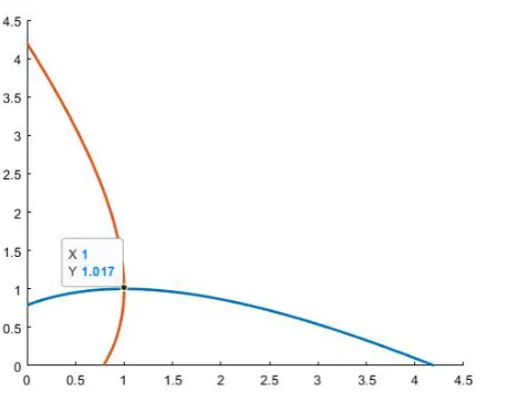
Figure 2: The unique Nash equilibrium is (E1∗, E2∗) = (1,1).
Since the above system is complicated based on the parametersr, q, P,C andK, to make a clearer analysis and easier understanding of the problem, we consider the following values for the parameters
r=P = 1, q=C = √1
27 and K = √
27.
In this case, the system (2.7) is
{
E1 = 3(((1 +E2) +
√
(1 +E2)2+ 1)
1
3 + ((1 +E2)− √
(1 +E2)2+ 1)
1
3)−1−E2
E2 = 3(((1 +E1) +√(1 +E1)2+ 1)13 + ((1 +E1)− √
(1 +E1)2+ 1)13)−1−E1
(2.8)
We have solved the above nonlinear system with the iterative method, that, as shown in Figure 2, it has an approximate unique solution (E1, E2) = (1,1), with very little error. This unique solution
is the Nash equilibrium of this model that we represent with (E1∗, E2∗) therefore (E1∗, E2∗) = (1,1). The total effort and harvest in the Nash equilibrium, ET and HT, are
ET =E1∗+E2∗ ∼= 1 + 1 = 2
and
HT =H1∗+H2∗
where
H1∗ =qE1∗( rK
(r+q(E1∗+E2∗)K))
2 =
√ 27
9 = 0.5773502691∼= 0.577 and similarly
H2∗ ∼= 0.577 then HT ∼= 1.15.
On the other hand, by substituting in (2.3) we have
HT =qET(
rK
(r+qETK)
)2 = √
27ET
(1 +ET)2
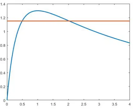
Figure 3: The functins HT = √
27ET
(1+ET)2, HT = 1.15 that the intersections of the two functions show
ET1, ET2.
But the recent relation is almost equivalent to
1.15ET2 −2.9ET + 1.15 = 0.
For this equation ∆ = 3.12 , √∆ = 1.7663521733 ∼= 1.77, and its roots are ET1 = 0.4913043478 ∼=
0.49 and ET2 = 2.0304347826∼= 2.03. (see Figure 3).
It should be noted that ET2 is approximately the sum of the levels of effort of the players in Nash
equilibrium and these two roots indicate that the amount of harvest in the Nash equilibrium can be obtained with ET2 and with less effort ET1. Since ET2 −ET1 ∼= 1.54, then in ET2 that players
are doing a static game with complete information thay are wasting 1.54 units of effort because the mass of fish is reduced and fishing is hardly done and players should spend more effort to harvest more. Therefore, by considering certain values as parameters, in order to make a clearer analysis, we conclude when the harvest function is nonlinear, doing a static game causes a waste of energy and money of both players. Therefore, doing a cooperative game with the agreement of the parties will be for the benefit of each player.
References
[1] Agnew, TT.,Optimal exploitation of a fishery employing a non-linear harvesting function, Ecological Modelling, Elsevier, 1979.
[2] Bernheim, BD., Rationalizable strategic behavior, Econometrica: Journal of the Econometric Society, JSTOR, 1984.
[3] Bischi, GI., Lamantia, F., Harvesting dynamics in protected and unprotected areas, Journal of Economic Behavior & Organization, Elsevier, 2007.
[4] Clark, CW., Restricted access to common-property fishery resources: a game-theoretic analysis, Dynamic opti-mization and mathematical economics, Springer, 1980.
[5] Clark, CW., Mathematical models in the economics of renewable resources, Siam Review, SIAM, 1979.
[6] Cohen, Y., A review of harvest theory and applications of optimal control theory in fisheries management, Canadian Journal of Fisheries and Aquatic ..., NRC Research Press, 1987.
[7] Cooke, KL., Witten, M., One-dimensional linear and logistic harvesting models, Mathematical Modelling, Else-vier, 1986.
[8] Dixit, AK., and Skeath, S., Games of Strategy, Fourth International Student Edition, 2015.
approach, Natural Resource Modeling, Wiley Online Library, 1998.
[14] Osborne, MJ., An introduction to game theory, Oxford University Press. New York, 2004. [15] Osborne, MJ., and Rubinstein, A., A course in game theory, MIT Press, 1994.
[16] Schaefer, MB., Some aspects of the dynamics of populations important to the management of the commercial marine fisheries, American Tropical Tuna Commission Bulletin, 1954.
[17] Schaefer, MB., Some considerations of population dynamics and economics in relation to the management of the commercial marine fisheries, Journal of the Fisheries Board of Canada, NRC Research Press, 1957.
[18] Sumaila, UR., A review of game-theoretic models of fishing, Marine policy, Elsevier, 1999.