ISSN: 2334-2986 (Print), 2334-2994 (Online) Copyright © The Author(s). All Rights Reserved. Published by American Research Institute for Policy Development DOI: 10.15640/jea.v5n1a2 URL: https://doi.org/10.15640/jea.v5n1a2
Statistical analysis of Impact of Building Morphology and Orientation on its Energy
Performance
Thulasi Ram Khamma1 & Mohamed Boubekri2
Abstract
Building energy consumption in developed countries accounts for 20–40% of the total energy use and about 40% of primary energy use in the U.S in 2010.Office buildings account for approximately 18% of this usage. The morphology of a building has a huge impact on its energy use, especially in office buildings due to their huge glazing areas. Designing with proper regard of climate issues leads to enhanced energy performance. This paper provides an analysis of the impact of building shapes and orientations on the energy performance across small, medium and tall office buildings for the Chicago, IL, USA location. The method is based on the analysis of simulation results obtained from energy modeling software, using Pearson Correlation and Multiple Linear Regression methods. The analysis considers six different building shapes; Rectangular (1:1, 1:1.5, 1:2), T, L and U. All of these considered shapes have identical construction and Window-wall ratios as specified in the Department of Energy (DOE) standard reference buildings. The aim is to establish a relationship between the impacts of building relative compactness (RC) on the energy performance of office buildings in three different cases: Small, Medium and Tall.
Keywords: Building Morphology, Relative Compactness, Energy performance, Internalloads and External
loads.
1.Introduction
The energy performance of a building relies heavily on the building shape and height, which are planned in the initial design phase. However, very little tools are available to architects to determine the balance between these two interdependent components; shape and height. Many studies were conducted to determine the relationship between the building morphology and its energy performance. This relationship varies widely with the location and operational characteristics of the facility. Building geometry, when properly determined according to the location and function, could result in substantial reduction of operational and energy costs. Building geometry can be illustrated by several simple numeric indicators; Volume-Area Ratio, Plan-Aspect Ratio, Section-Aspect Ratio, and other. Generally, these indicators are generated through the internal volume and external surface area. They indirectly represent internal and external loads in a building. [Mahdavi and Gurtekin 2002] introduced the concept of “Relative Compactness” as a measure of the geometrical compactness of the building. It seems to be very effective in comparison studies to assess the impact of building shape and energy performance, as shown by [AlAnzi et al. 2009a; Ourghi et al. 2007a] The behavior of energy loads in buildings vary with the height and shape of the building due to the change in the balance of internal and external loads.
Studies have demonstrated that the building shape can have significant impact on the heating and cooling loads of the building [AlAnzi et al. 2009a; Ourghi et al. 2007a]. These studies have developed simplified tools and methods to predict the impact of the shape on the energy efficiency of the buildings. Particularly studies by [Ourghi et al. 2007a; Danielski et al. 2012; Depecker et al. 2001a] were focused on establishing relationships between the building compactness and energy consumption. The aim of this research study is to analyze the varying influence of cooling and heating loads with the building height and relative compactness on the energy loads of the building. Most of the recent research studies sought to identify the relationship between the RC or building volume and Building energy loads [ Parasonis et al. 2012; Pessenlehner and Mahdavi 2003; Ratti et al. 2003]. They either had considered hypothetical building shapes with constant floor area with constant height or constant floor area with varying height among different shapes or modular shapes. But, our study is based on standard office building floor areas and heights defined by the Department of Energy’s (DOE) commercial reference buildings. These buildings have 16 types that represent approximately 70% of the commercial buildings across 16 locations representing all U.S. climate zones.
1.1 Relative Compactness (RC)
The shape of a building is best explained by its internal volume and external surface area. Through their studies, [Mahdavi and Gurtekin 2002], concluded that RC is a better measure of the subjective categorization of shape compactness by designers. Since the shape samples used in our study are of equal volume, we conclude that RC would be an ideal measure of comparison.
RC is an indicator of the building’s geometric compactness. Buildings with high RC are more compact and vice versa. RC, a shape-dependent factor, is generated by comparing the volume to surface ratio of the building to that of a cube with identical volume. Here, the surface area includes the entire area that is exposed to the outside environment, i.e, the sum of the walls, roof and the ground floor areas. The higher the RC value the more compact the building is.
RC = =(Surface Area)
(Surface Area)
1.2 Building Orientation (OR)
Orientation is a huge factor in case of office buildings (chosen building type) which have majority of wall area covered with glass windows. This extensive glazing offers spectacular views and daylighting while resulting in increased energy consumption for heating and cooling due to their weak thermal resistance. Hence, the orientation of a building on site is one of the deterministic factors of the amount of heat gains and losses. Selecting an optimal orientation would have influence the energy consumption of a building positively.
1.3 Building Type & Location
It is the one of the major cities in the East North Central region of United States, which accounts for approximately 21% of the total energy end usage in the US. Office buildings account for approximately 19% of these total energy usage. Hence, studying the impact of building morphology in this building type and location would have a huge impact on the future architectural design and energy usage. Future analyses will include other climatic regions.
2 Methodology
Our analysis is based on results obtained from building energy model simulations. Building energy modeling is the process of virtually recreating the physical building replicating all of its characteristics and by taking the climate into consideration. They provide valuable insights to designers and engineers on the behavior of the thermal loads in the buildings based on their architecture, operation type, internal activities and loads, and construction materials, and are often used to evaluate alternatives in building design. This study employs building energy simulations to study the impact of different building shapes, orientations and heights on the thermal loads in Office buildings.
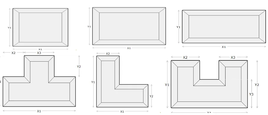
2.1Shapes and Dimensions
The office buildings are modeled with six typical shapes employed in the architectural design. Three rectangular shapes with sides’ ratio of 1:1, 1:1.5 and 1:2, ‘L’, ‘T’ and ‘U’ shapes were modeled for our study as shown in Figure 1 based on the office building floor areas and heights defined by the Department of Energy’s (DOE) commercial reference building types including Small, Medium and Tall offices. Models were developed for these three building types, to ascertain the energy behavior of the office buildings at different heights. The floor areas for these shapes are adopted from the standard reference buildings for energy modeling. The shape characteristics and dimensions for the small, medium and tall buildings are provided in the Table 1, Table 2 and Table 3 respectively.
Table 1 - Shape characteristics of Small office building models
Shape RC Area
(Sq.ft) No. of Floors Floor-Floor height (ft.) Percent of perimeter zone area Volume (Cu.ft) X1 (ft) X2 (ft) X3 (ft) Y1 (ft) Y2 (ft) Y3 (ft) Rectangle (1:1)
0.6730 5,500 1 12 64.5 14,600 74.15 - - 74.15 - -
Rectangle (1:1.5)
0.6696 5,500 1 12 66.2 14,600 90.85 - - 60.55 - -
Rectangle (1:2)
0.6632 5,500 1 12 69.4 14,600 104.90 - - 52.45 - -
T 0.6416 5,500 1 12 78.4 14,600 101.35 29.85 41.65 72.40 30.75 -
L 0.6340 5,500 1 12 80.7 14,600 89.00 39.80 - 89.00 39.80 -
U 0.6459 5,500 1 12 84.9 14,600 98.95 37.00 37.00 61.85 61.85 37.00
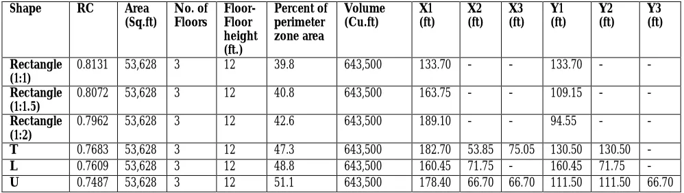
Table 2 - Shape characteristics of Medium office building models
Shape RC Area
(Sq.ft) No. of Floors Floor-Floor height (ft.) Percent of perimeter zone area Volume (Cu.ft) X1 (ft) X2 (ft) X3 (ft) Y1 (ft) Y2 (ft) Y3 (ft) Rectangle (1:1)
0.8131 53,628 3 12 39.8 643,500 133.70 - - 133.70 - -
Rectangle (1:1.5)
0.8072 53,628 3 12 40.8 643,500 163.75 - - 109.15 - -
Rectangle (1:2)
0.7962 53,628 3 12 42.6 643,500 189.10 - - 94.55 - -
T 0.7683 53,628 3 12 47.3 643,500 182.70 53.85 75.05 130.50 130.50 -
L 0.7609 53,628 3 12 48.8 643,500 160.45 71.75 - 160.45 71.75 -
U 0.7487 53,628 3 12 51.1 643,500 178.40 66.70 66.70 111.50 111.50 66.70
Table 3 - Shape characteristics of Tall office building models
Shape RC Area
(Sq.ft) No. of Floors Floor-Floor height (ft.) Percent of perimeter zone area Volume (Cu.ft) X1 (ft) X2 (ft) X3 (ft) Y1 (ft) Y2 (ft) Y3 (ft) Rectangl e (1:1)
0.9457 498,58 8
12 + basement
13 28.3 5,983,000 195.8
5
- - 195.85 - -
Rectangl e (1:1.5)
0.9335 498,58 8
12 + basement
13 28.9 5,983,000 239.8
5
- - 159.90 - -
Rectangl e (1:2)
0.9107 498,58 8
12 + basement
13 30.1 5,983,000 276.9
5
- - 138.50 - -
T 0.8559 498,58
8
12 + basement
13 33.5 5,983,000 267.6
5
78.8 5
109.95 191.15 81.25 -
L 0.8394 498,58
8
12 + basement
13 34.4 5,983,000 235.0
0
105. 10
- 235.00 105.10 -
U 0.8165 498,58
8
12 + basement
13 36.0 5,983,000 261.3
5
97.6 5
97.65 163.35 163.35 97.6
5
This strategy ensures close representation of actual systems and also reduce the possibility of unmet loads in the energy model.
2.2 Construction Details
Identical construction specifications for climate zone 5A in ASHRAE 90.1 were used for all the office building models in three different height categories. The construction details for all the models are detailed in Error! Not a valid bookmark self-reference. according to the ASHRAE 90.1 standard and DOE commercial reference buildings.
Table 4–Construction details of the models
Shape Roof Type
Roof
Construction(R-Value in Hr-Sqft-F°/ Btu) Wall Construction Floor Construction Doors(U-value in Btu/Hr-Sqft-F°) Windows(U-value in Btu/Hr-Sqft-F°)
Small Office Attic roof Metal Building (R-13 +R-13)
Metal Building (R-13 +R-5.6 c.i)
- Double glazing with thermal break (U-value = 0.52) Double glazing with thermal break (U-value = 0.52) Medium Office
Flat roof Metal Building (R-13 +R-13)
Metal Building (R-13 +R-5.6 c.i)
Mass floors (R-10.4 c.i) Double glazing with thermal break (U-value = 0.52) Double glazing with thermal break (U-value = 0.52)
Tall Office Flat Roof Metal Building (R-13 +R-13)
Metal Building (R-13 +R-5.6 c.i)
Mass floors (R-10.4 c.i) Double glazing with thermal break (U-value = 0.52) Double glazing with thermal break (U-value = 0.52)
2.3 Internal and External Loads
Latent heat is the heat that causes the change in the moisture content of the space whereas the sensible heat is the heat that causes change in the temperature of the space. The total heat gain is the sum of both of these. People, equipment and infiltration are the main sources that influence latent heat in a building, whereas the heat through different sources like the wall, roof, doors, windows, people and equipment, impact the sensible heat. Internal loads constitute both the latent and sensible heat gains from people, lighting, equipment and process loads. These loads are dependent on the building type and its operational schedules. They are dependent on the floor area of the building. External loads include the heat gains occurring by heat transfer mechanisms; conduction, convection and radiation, through external walls, roof, ground surface, doors and windows. These loads are dependent on the environmental factors, like climate and location as well as the configuration of building components. They vary with the change in the surface area of the building. Both internal and external loads combine together to form Cooling Load (CL) and Heating Load (HL).
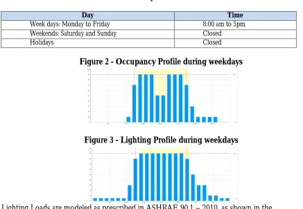
Typical operational profile of an office building is modeled as shown in the Table 5. These operational timings are followed for the occupancy, lighting and equipment schedules.
Equipment loads during this time vary based on the occupancy of the space. Occupancy and lighting profiles vary during the weekdays as shown in the
Figure 2 and Figure 3 respectively.
Table 5–Operational Profile
Day Time
Week days: Monday to Friday 8:00 am to 5pm Weekends: Saturday and Sunday Closed
Holidays Closed
Figure 2 - Occupancy Profile during weekdays
Figure 3 - Lighting Profile during weekdays
Lighting Loads are modeled as prescribed in ASHRAE 90.1 – 2010, as shown in the
Table 6 below.Daylighting was not considered in the models, since it was not a criteria for this study.
Table 6–Lighting loads
Space Lighting (W/S.ft)
Office (Open plan) 0.98
Office (Executive/Private) 1.11
Corridor 0.66
Lobby 0.90
Conference 1.23
Copy room 1.50
Restrooms 0.98
Mechanical / Electrical Rooms 1.50
Energy. This software runs on the DOE-2 engine. Each individual model is oriented at four different orientations; 0°, 90°, 180° and 270° with respect to Sun’s position. 0° orientation is considered to be the base model with the longest side facing south. So, each height category results in 24 different models. Simulations results, which include both the heat and cool loads, for all the models in each height category are analyzed together using statistical analysis methods: Pearson correlation coefficient and Multiple Linear Regression.
2.4 Statistical analysis methods
The study uses Pearson correlation analysis to measure the strength of the linear association between the RC and cooling and heating loads. Correlation analysis focuses on the strength of the relationship between multiple variables whereas regression analysis assumes a causal relationship and generally used to identify the strength of effect by multiple independent on one dependent variable. Multiple linear regression (MLR) attempts to model the relationship between multiple predictor variables and a response variable by fitting a linear equation to observed data. Hence, the study uses MLR method to further analyze this linear relation between these variables.
2.4.1 Pearson correlation coefficient
Pearson correlation coefficient which lies in between -1 and 1, is a measure of the strength of linear correlation between two variables. Positive values indicate weight of the positive correlation where 1 indicates absolute positive correlation. Whereas the negative values indicate the strength of negative correlation where -1 indicates absolute negative correlation. It is obtained by calculating the covariance of the two variables divided by their standard deviations. Pearson correlation coefficient for any two variable x and y is given by:
, =
( , )
, is the Pearson correlation coefficient, is standard deviation of x and is standard deviation of y.
2.4.2 Multiple Linear Regression (MLR)
MLR consists of Response variable, Predictor variables, their interactions and error term. It is most commonly used to estimate the linear relationship between the response and two or more predictors. These predictors could be categorical or continuous in nature, sometimes a mixture of both. The model assumes that the data follows a Gaussian distribution, linear relationship between the response and predictor variables, absence of multicollinearity among the predictors, and error terms are homoscedastic (constant variance). The simplest form of MLR with two predictors and interaction term is defined as:
= + ∗ + ∗ + ∗ ∗ +
yi is the response variable, is the intercept, and are the coefficients of the predictor variables, is the coefficient of the interaction between the
two predictor variables and is the error term or residual.
Since the coefficients change with the predictors, the effect of each of the predictors are no longer constant. Changing one predictor will alter the impact of the other on Y. If either one of the predictors are insignificant, then they can be removed from the model since they do not explain the variation in the response variable. Suppose if X2 and the interaction term are not significant then the resulting model will
line. In other words, the least squares approach is to minimize the sum of squared error terms. Our null hypothesis in this MLR analysis is that a predictor variable is significant in predicting the response. Alternative hypothesis is that the null hypothesis is false. The p-value is used to determine the significance of the results. A small p-value indicates strong evidence against null hypothesis and null hypothesis is rejected.
Alternatively, if p-value is large, null hypothesis is not rejected. This hypothesis testing involves setting up a threshold value for p, called significance level or α. If the p-value is less than or equal to the chosen α, the test indicates that the null hypothesis must be rejected. Typically, p-value is less than or equal to 0.05 is accepted as the desired cutoff at α=95% significance level. A variable is said to be significant if the p-value is less than 0.05 at α=95% significance level. The p-value in the MLR results indicate that if a variable is significant or not in predicting the response variable. The study chooses α = 95% level and p -value <=0.05 to assess the MLR results.
3 Results
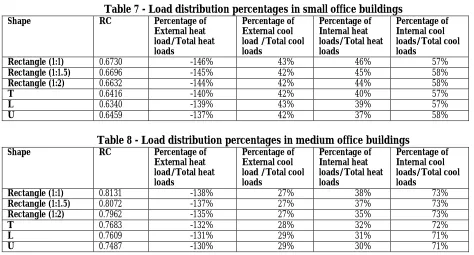
The internal and external loads for all shapes at 0° orientation, are broken down from the simulation results. As mentioned earlier, internal loads include the heat gains from people, equipment, lighting and process loads. They are constant across all shapes of in each height category since their floor areas remain the same but their percentage with respect to the total load changes based on the change in the external loads. Thepercentage of external heat load to total heat loadis treated as negative since they constitute heat losses and internal loads as positive since they add heat to the space. The breakdown of the internal and external loads among the three categories are as follows:
Table 7 - Load distribution percentages in small office buildings
Shape RC Percentage of
External heat load/Total heat loads
Percentage of External cool load /Total cool loads
Percentage of Internal heat loads/Total heat loads
Percentage of Internal cool loads/Total cool loads
Rectangle (1:1) 0.6730 -146% 43% 46% 57%
Rectangle (1:1.5) 0.6696 -145% 42% 45% 58%
Rectangle (1:2) 0.6632 -144% 42% 44% 58%
T 0.6416 -140% 42% 40% 57%
L 0.6340 -139% 43% 39% 57%
U 0.6459 -137% 42% 37% 58%
Table 8 - Load distribution percentages in medium office buildings
Shape RC Percentage of
External heat load/Total heat loads
Percentage of External cool load /Total cool loads
Percentage of Internal heat loads/Total heat loads
Percentage of Internal cool loads/Total cool loads
Rectangle (1:1) 0.8131 -138% 27% 38% 73%
Rectangle (1:1.5) 0.8072 -137% 27% 37% 73%
Rectangle (1:2) 0.7962 -135% 27% 35% 73%
T 0.7683 -132% 28% 32% 72%
L 0.7609 -131% 29% 31% 71%
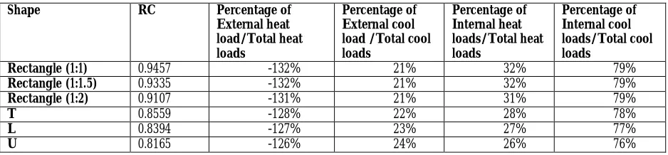
Table 9- Load distribution percentages in tall office buildings
Shape RC Percentage of
External heat load/Total heat loads
Percentage of External cool load /Total cool loads
Percentage of Internal heat loads/Total heat loads
Percentage of Internal cool loads/Total cool loads
Rectangle (1:1) 0.9457 -132% 21% 32% 79%
Rectangle (1:1.5) 0.9335 -132% 21% 32% 79%
Rectangle (1:2) 0.9107 -131% 21% 31% 79%
T 0.8559 -128% 22% 28% 78%
L 0.8394 -127% 23% 27% 77%
U 0.8165 -126% 24% 26% 76%
There appears to be a slight variation in the percentage of external cool loads to the total cool loads across the different shapes in the case of small office buildings as indicated in table 7. It varies more in both medium and tall buildings (Table 8 & 9). Both the percentages of external cool load to the total cool load, and external heat load to the total heat load are larger for small office buildings and decrease gradually with the height of the building. The cooling and heating loads are considered for further analysis in each height category and are treated as response variables in MLR models.
3.1 Correlation Analysis
The Pearson correlation coefficient indicate higher correlation factors (ŕ) among all the models with RC in case of heating load. For cooling load, ŕ varies widely across the three categories. It is very weak and negligible in the small buildings and stronger in the tall buildings category.
Table 8: Correlation coefficient between RC v/s CL v/s HL across small, medium and tall categories
Category CL HL
Small 0.281 -0.994
Medium -0.713 -0.998
Tall -0.944 -0.998
3.2 MLR Results
Two separate MLR models for cooling and heating loads were developed with RC and OR as predictor variables to analyze the impact of the predictor variables on the response variables. These models were developed utilizing R statistical software. RC is treated as a continuous variable whereas OR is treated as categorical variable. The cooling and heating loads are divided by constant, 106 for easy interpretation of the models, since scaling them would not alter the results of the MLR analysis. The analysis of MLR results for small office buildings indicates that Relative Compactness (RC) is insignificant (at α = 95% level and p-value <=0.05) in predicting the cooling load, i.e., it does not vary much with change in RC. The resulting equations suggest that the heating load decreases at the rate of approximately
0.5 times and cooling load has a negative impact with a change in the OR. The resulting MLR equations for cooling and heating loads for small office building models are as follows:
The results from MLR suggest that increasing RC by 1 unit will result in decreasing cooling load by approximately 0.6 times and heating load by 1.5 times. The resulting equations for cooling and heating loads for medium office building models are as follows:
= 2.298−0.587∗ + 0.016 (90° )−0.002 (180° ) + 0.016 (270° ) = 1.539−1.448∗
The results from MLR indicate that in tall buildings, cooling load and heating load decreases at approximate rates of 4 and 4.4 times respectively, with one-unit increase in RC. The resulting equations for CL and HL for tall office building models are as follows:
= 19.903−4.021∗ + 0.097 (90° )−0.005 (180° ) + 0.093 (270° ) = 6.328−4.369∗
The following table summarizes the impact of RC on cooling and heating loads among the different height categories.
Category Rate of change in CL Rate of change in HL
Small - -0.5*RC
Medium -0.6*RC -1.5*RC
Tall -4.0*RC -4.4*RC
4. Conclusions
Our study proposes a methodology to study the relationship between the relative compactness and energy loads in the building across three building height categories. It is based on the office building floor areas and heights defined by the Department of Energy’s (DOE) commercial reference buildings.
We can conclude the following on the relationship between the RC and cooling and heating loads across the three height groups:
The results suggest that Orientation seems to have very little or negligible effect on the energy loads of an office building in this climate.
As the building becomes more compact, the cooling loads for tall office buildings decreases at a higher rate than the medium size or small size categories. The RC seems to have negligible impact on the cooling loads of a small office building.
As the building becomes more compact, the heating load for tall office buildings decreases at a faster rate than the other two size categories.
The impact of RC increases on the heating load with the increase in the height.
The correlation analysis and the MLR models suggest that there is strong negative correlation between the RC of the building and heating load in the three building categories i.e., the more compact the building is the lesser the heating load will be in this climate.
5. Limitations
6. References
Adnan AlAnzi, Donghyun Seo, and Moncef Krarti. 2009a. Impact of building shape on thermal performance of office buildings in Kuwait. Energy Convers. Manag. 50, 3 (March 2009), 822–828. DOI:http://dx.doi.org/10.1016/j.enconman.2008.09.033
Anon. Energy Information Administration (EIA)- Commercial Buildings Energy Consumption Survey (CBECS) Data.Retrieved April 18, 2016 from http://www.eia.gov/ consumption/ commercial/ data/2003/
Itai Danielski, Morgan Fröling, and Anna Joelsson. 2012. The impact of the shape factor on final energy demand in residential buildings in nordic climates. In World Renewable Energy Forum, WREF 2012, Including World Renewable Energy Congress XII and Colorado Renewable Energy Society (CRES) Annual Conference; Denver, CO; 13 May 2012through17 May 2012; Code94564. 4260– 4264.
Patrick Depecker, Christophe Menezo, Joseph Virgone, and Stephane Lepers. 2001a. Design of buildings shape and energetic consumption. Build. Environ. 36, 5 (2001), 627–635.
Ardeshir Mahdavi and Beran Gurtekin. 2002. Shapes, Numbers, and Perception: Aspects and Dimensions of the Design Performance Space. In Proceedings of the 6th International Conference: Design and Decision Support Systems in Architecture. Ellecom, The Netherlands. ISBN. 90–6814.
Ramzi Ourghi, Adnan Al-Anzi, and Moncef Krarti. 2007a. A simplified analysis method to predict the impact of shape on annual energy use for office buildings. Energy Convers. Manag. 48, 1 (January 2007), 300–305. DOI:http://dx.doi.org/10.1016/j.enconman.2006.04.011
Josifas Parasonis, Andrius Keizikas, Audronė Endriukaitytė, and Diana Kalibatienė. 2012. Architectural Solutions to Increase the Energy Efficiency of Buildings. J. Civ. Eng. Manag. 18, 1 (February 2012), 71–80. DOI:http://dx.doi.org/10.3846/13923730.2011.652983
Werner Pessenlehner and Ardeshir Mahdavi. 2003a. Building morphology, transparence, and energy performance, na.
Carlo Ratti, Dana Raydan, and Koen Steemers. 2003. Building form and environmental performance: archetypes, analysis and an arid climate. Energy Build. 35, 1 (2003), 49–59.