ISSN: 2334-2986 (Print), 2334-2994 (Online) Copyright © The Author(s). All Rights Reserved. Published by American Research Institute for Policy Development DOI: 10.15640/jea.v4n2a5 URL: https://doi.org/10.15640/jea.v4n2a5
How Accurate are Travel Forecasts: Back Casting of Truck Lane Restrictions using
Multi-Resolution Modeling Methods
Jeffrey Shelton
1, Gabriel A. Valdez
2& Peter Martin, PhD., P.E.
3Abstract
The integration of mesoscopic and microscopic simulation models provide expanded dimensions of modeling capabilities by taking the strengths of both model resolutions. Many transportation agencies, practitioners and researchers are beginning to see the advantages of using multiple levels of resolution when analyzing corridor specific problems. Mesoscopic models use dynamic traffic assignment to reroute traffic given various traffic conditions. Microscopic models are used to analyze traffic conditions at the individual car or lane level. Models are calibrated and validated using data collected in the field. Most practitioners validate their models to existing conditions and then forecast future conditions to predict traffic congestion. Once simulation runs are finished, results are presented to hosting transportation agencies and the project is completed. Very few practitioners collect future field data and compare it to the simulated forecasts. This sort of reverse model validation is referred to as back casting. This paper outlines the complete modeling process from model development, conversion, calibration, consistency, validation and ultimately - model back casting. A case study involving user class restrictions on Interstate 10 in El Paso, Texas was used to analyze how accurate the models were at predicting future conditions. Researcher’s simulated truck restricted lanes on the freeway to determine how effective the user class restrictions were on overall traffic speeds and travel times. One year later when the truck lane restrictions were in place, field data was collected to determine how accurate the models were at predicting traffic conditions.
Keywords: Backcasting, Multi-Resolution Modeling, Mesoscopic, Microscopic, Dynamic Traffic
Assignment, Validation
1. Introduction
Traffic analysts and operating agencies increasingly rely on traffic analysis tools to analyze and evaluate the current and future performance of transportation facilities for various modes of transport. There are a variety of software-based analytical procedures and methodologies developed by public agencies, research organizations, and private consultants that support different aspects of traffic and transportation analyses. These analyses usually rely on modeling software to assess the performance of transportation facilities.
These models are classified based upon their level of resolution and can be categorized as macroscopic, mesoscopic or microscopic. For long range planning projects, macroscopic tools analyze in a simplistic manner and at an aggregate level.
However, this type of static representation of traffic fails to capture the intricate details of real-life conditions such as the fluctuation of traffic build-up and dissipation during peak-hour congestion periods and therefore cannot predict network performance temporally. Long-range planning models are geared for such applications because there is no need to analyze the interaction of vehicles at a more refined level. Microscopic simulation models in contrast describe the system entities and a high level of detail. The details of microscopic models yield the flexibility to add many more modeling contexts and options than mesoscopic and macroscopic models- but are limited in size and require an abundance of calibration parameters. Mesoscopic simulation and assignment models fill the gaps between the aggregate level approach of macroscopic models and the individual interactions of the microscopic ones. Mesoscopic models normally describe the traffic entities at a high level of detail, but their behavior and interactions are described at a lower level of detail[1].
Incorporating multiple-levels of resolution often includes the integration of model platforms. Model integration is fast becoming a simulation modeling approach since it takes both the localized and system-wide analyses into consideration. In the existing practice, these types of models are often used jointly in a traffic analysis; however, the actual practice and use of these models may vary widely among different analysts or regions. Practitioners often establish their standard practices through experience or at times the requirements from the transportation agency clients. On the other hand, transportation agencies may or may not establish the model use guidelines, and if they do, the standards often vary.
Within the context of multi-level resolution comes the practice of model validation. Validation normally refers to authenticating model results to existing conditions. This is usually done using existing data collected in the field and trying to match simulated results with collected data. Hawas stated that the purpose of model validation is to ensure that the simulation model accurately represents the real world[2]. The Florida Department of Transportation (FDOT) initiated a study of best practices for model calibration and validation. FDOT described model validation as a procedure used to adjust models to simulate base year traffic counts and transit ridership figures for their travel demand models and that it consists of reasonableness and sensitivity checks beyond matching base year conditions [3].
While there is extensive literature on model validation as it relates to existing conditions, there are few studies that actually take field data from future years and validate how accurate the simulation models were. This is due in part to budgeting constraints. Project budgets are calculated based upon the amount of effort needed to perform a transportation study which typically included data collection, model development, calibration, validation and final analyses. This type of analysis can be considered a one directional process. Once model results have been obtained and presented to hosting transportation agencies, recommendations are given and usually implemented under normal circumstances. There are very few instances when data is collected after a project has been completed and compared to the forecasted results.
The objective of this study was to perform a back casting analysis using a previously developed case study in El Paso, Texas where city council wanted to implement truck lane restrictions on Interstate 10 (I-10). The case study main objective was to develop a simulation based analysis to quantify the impact on vehicles speed with and without truck lane restrictions on I-10. In order to do so, the researchers collected field data which was used in the model development and calibration process.
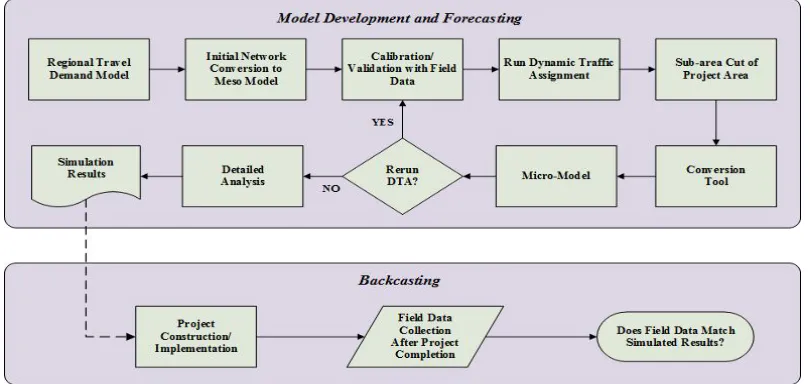
Once models were calibrated and validated, simulation results were obtained and presented to the Texas Department of Transportation (TxDOT). Shortly after simulation results were presented to TxDOT, the El Paso city council approved the ordinance and the user class restrictions went into effect. One year after these restrictions were in place, researchers went back and collected field data to determine how accurate the simulation models were at predicting the outcome of the truck lane restriction ordinance. The following sections outline the entire modeling process used in this study from initial model conversion, development, calibration and forecasting, to the final back casting analysis as shown in Figure 1.
Figure 1: Model Development, Forecasting and back casting Process
Research methodology
Multi-Resolution Modeling
Macroscopic to Mesoscopic
The process begins with the conversion of the TDM to mesoscopic format. In addition, the regional model has an aggregated origin/destination (OD) matrix that is composed of all combined trip purposes. The origin/destination (OD) matrix is disaggregated where each corresponding trip purpose matrix is multiplied by corresponding hourly factor that is provided by the MPO as shown in Figure 2.
Figure 2: Origin-Destination Matrix Development
Once all trip purposes are multiplied by hourly factors, the matrices are summed which in turn provides a one-hour matrix with directionality in mesoscopic format. The process is repeated for all additional hourly factors in a 24-hour period. The formulation for matrix conversion is expressed as:
φ δ ∀ k∈
ℎ :
=ℎ ℎ
=
= ℎ ℎ 24 ℎ
∈ { , , , , − , }
HBW = Home-based to work
HBNW = Home-based to non-work
TRTX = Truck/taxi
NHB-V = Non-resident trips made by external local travelers
EXLO = External local
Mesoscopic Calibration
After the conversion process is completed, it is necessary to calibrate the mesoscopic traffic flow model with collected field data. The traffic simulation in DynusT is based on an anisotropic mesoscopic simulation (AMS) model, which is built upon the intuitive concept that at any time, a vehicle’s prevailing speed is affected only by vehicles in front of it; including those in the immediate adjacent lanes[4]. It is necessary to determine the maximum density (i.e. jam density) that sustains free-flow speed on freeway corridors. Green shield’s equation is used to calibrate the speed-density (v-k) relationship within the AMS model using field data. Several trial and error inputs for minimum speed, free flow speed and intercept speed were used to determine optimal jam density. The optimal jam density was ultimately determined by matching the corresponding observed v-k relationship to the calibrated as shown in Figure 3.
Figure 3: Flow-Density relationship
After all traffic models have been derived, it is necessary to calibrate the converted OD. It is calibrated based upon data collected in the field in the form of traffic counts (cars and trucks). The OD calibration process uses a linearized quadratic minimization problem developed by the University of Arizona where simulated link counts (volumes) are compared with real traffic data collected in the field. The program minimizes the deviation between simulated and actual screen line counts and updates OD pairs during each iteration until it reaches a predefined threshold[5].
Figure 4: OD Linear Minimization Optimization Process
Once the mesoscopic model has been calibrated with collected field data, it is run to UE conditions using DTA. DTA is a time-dependent process that captures traveler’s route choice behavior as vehicles travel from origin to destination. The objective function known as dynamic user equilibrium (DUE) is based on the idea of drivers choosing their routes through the network according to a “generalized” travel cost which consists of monetary costs (tolls) and experienced travel time. The DUE process is an iterative process where travelers learn and adapt to the network conditions[6]. Part of the generalized cost calculation uses the value-of-time (VoT) to assess the time-dependent shortest path when running traffic assignment. However, while VoT is a very important notion in simulation-based modeling, it is a latent theoretical constructed value that cannot be easily quantified[7].
Therefore it is imperative that an accurate calculation of VoT be used as part of the generalized cost calculation- otherwise routing of vehicles can (especially for toll roads) can vary tremendously. For this study, the VoT was taken from the official travel demand model used for conformity purposes. Automobiles were assigned a VoT of $14.00 while freight (trucks) was given a higher value at $30.00.In addition, separate truck demand matrices were used to replicate realistic travel patterns for both modes of transportation; auto and freight. This was necessary to prevent unwarranted or unrealistic travel patterns of trucks (e.g. substantial amount of truck traffic on a university campus, central business district).
Model Conversion
Figure 5: Model conversion process
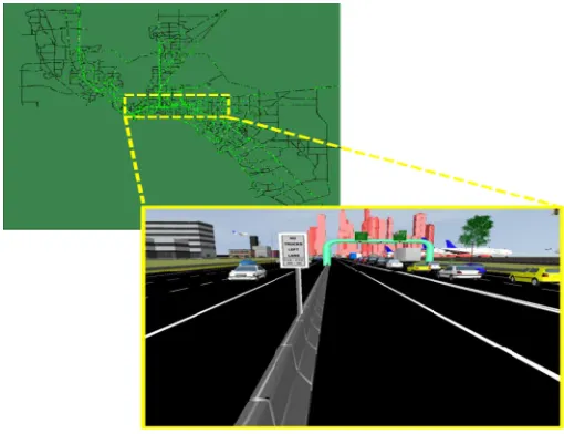
Time-dependent paths and flows were transferred from the Dynus T model to VISSIM for the three different defined time-periods. It was necessary to convert the mesoscopic model to a microscopic counterpart because of the level of detail necessary for this analysis.
Mesoscopic models cannot analyze the interactions of individual vehicles on separate lanes. Microscopic models are capable of this type of analysis but cannot replicate OD zones on a network of this size with any consistency. The VISSIM models then allows for a more “fine-grained” analysis of vehicle interactions at the localized level and ultimately determine whether or not truck restricted lanes benefit traffic congestion within the project limits.
Microscopic Model Input
Data was collected at strategic locations on I-10 and used as input for model calibration. A Global Positioning System (GPS) unit was used to determine altitudes for various segments of I-10. Altitude measurements were then used to determine grading along the freeway corridor. Input of grading in the microscopic model is necessary as if affects acceleration and deceleration patterns of all vehicles within the network. Each positive/negative percentage point adjusts the acceleration/deceleration of vehicles by 0.328 ft/s2[8]. Stations were determined by X-Y coordinates from Google maps© where high and low point segments of the freeway were determined from the GPS output. Due to the wide range of speed distributions along the freeway corridor, it was necessary to create multiple vehicle classifications for large commercial trucks. Previous research [9] was the guide in determining what types of trucks were typically found in Texas and what percentage of the truck traffic stream each comprised. The source of these data were the Tx DOT Automatic Traffic Recorder (ATR) Stations which record traffic volumes and classification on a year-round basis and provide permanent historical records of traffic conditions.
Table 1: Truck Characteristics Applied to Texas Truck Fleet
Truck Class
Relative Flow
Length (ft)
Width (ft)
Weight (lb) Power (hp)
Min. Max. Min. Max.
5 0.004 27.89 8 15,000 46,000 220 260
6 0.001 27.89 8 20,000 53,000 220 300
7 0.000 30.94 8 25,000 52,000 250 300
8 0.001 36.13 8 28,000 66,000 315 380
9 0.042 60.22 8 30,000 80,000 380 480
10 0.000 55.39 8 32,000 87,000 415 490
11 0.002 70.69 8 35,000 92,000 440 500
12 0.040 67.24 8 35,000 106,000 505 525
13 0.000 92.35 8 35,000 120,000 570 580
Microscopic Calibration
A radar gun was used to determine the average speed profiles of large commercial trucks. The speed profile was calibrated from actual field data collection in terms of both traffic volumes and speeds on the freeway corridor. This was needed to calculate the queue lengths for freeway facilities based upon an assumed linear relationship between density and flow[11]. It was also necessary to perform a series of screen line counts to validate the entry volumes at specific freeway on-ramps as shown in Figure 6.
A final visual inspection of the models was performed to identify any potential inconsistencies within the network. If any inconsistencies that occur during the conversion process (e.g. incorrect number of lanes on freeway corridor) that would cause vehicles to change their respective routes, then changes must be reflected in the DynusT model and DTA must be rerun. When the microscopic model is developed and calibrated to satisfaction, a series of detailed analyses are performed. A base model was used for comparative purposes where trucks were free to travel in all lanes. A second model was duplicated with trucks restricted from the left-most fast lane. Speeds and travel times were compared for each defined time period.
Forecasted Analysis
Morning Peak Hour (7-11 AM)
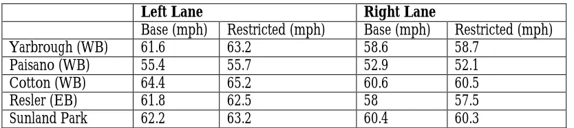
The morning peak hour simulation model was run for 4-hours from 7-11 am. The model had 122 static routing decisions and 2144 routes created for both auto and trucks. Traffic volumes and routes were updated every 15 minutes for the entire simulation period. Simulation outputs were calculated every 5 minutes and included average speed, acceleration/decelerations, and travel time for both the eastbound and westbound directions. Data collection points were determined based upon areas of recurring traffic congestion. Average speeds (mph) were collected for both the left and right lanes respectively as shown in Table 2. It must be noted that several random seeds were used and data output was averaged for all modeled scenarios.
Table 2: Average Speed (7-11 am)
Left Lane Right Lane
Base (mph) Restricted (mph) Base (mph) Restricted (mph)
Yarbrough (WB) 61.6 63.2 58.6 58.7
Paisano (WB) 55.4 55.7 52.9 52.1
Cotton (WB) 64.4 65.2 60.6 60.5
Resler (EB) 61.8 62.5 58 57.5
Sunland Park 62.2 63.2 60.4 60.3
Simulation results showed increased speeds on the left lane on I-10 that ranged from 0.3 to 1.6 mph in most locations. Right lane speed decreased slightly after the restrictions with the Paisa no area experiencing the highest average speed decrease at -0.8 mph. Travel time was also calculated for both the east and west bound directions of I-10. For vehicles traveling on I-10 eastbound, travel time was averaged from N. Mesa St (SH 20) to Schuster Ave (exit ramp18A) and N. Mesa St (SH 20) to N. Lee Trevino Dr (exit ramp 29). For vehicles traveling on I-10 westbound, travel time was averaged from Lee Trevino Blvd to E. Missouri Ave (exit ramp 19B) and N. Lee Trevino Dr to Redd Rd (exit ramp 10). Travel times were almost identical for both the base and restricted scenarios in the east and westbound directions.
Mid-day (11-3 PM)
The mid-day simulation model was run for four hours from 11 am to 3 pm. Data collection was taken at various locations during the simulation. Results showed that average speeds increased at all locations during the mid-day simulation with the exception of I-10 at Schuster Ave westbound where there was no improvement. I-10 at McRae eastbound showed the highest improvement in average speed with a +2.1 mph improvement over the base case model. I-10 at Yarbrough eastbound showed a +1.8 mph improvement, while I-10 at Resler eastbound showed a +1.3 mph improvement with trucks restricted from the left-most lanes.
In the eastbound direction, vehicles traveling from N. Mesa St to Lee Trevino Dr had an average improvement of 12 seconds while traveling in the westbound direction had a 6-12 second improvement in travel time on the freeway.
Table 3: Average Speed (11-3 PM)
Left Lane Right Lane
Base (mph) Restricted (mph) Base (mph) Restricted (mph)
Yarbrough (WB) 61.9 63.7 58.9 59.2
Paisano (WB) 58.2 58.8 53.6 52.4
Cotton (WB) 65.2 65.6 60.6 60.7
Resler (EB) 62.8 64.1 59.3 59.4
Sunland Park (EB) 63.0 63.8 60.7 60.5
Afternoon Peak Hour (3-7 PM)
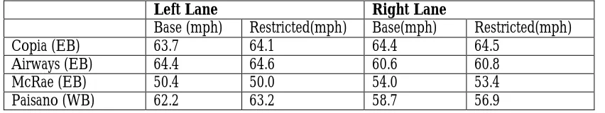
The afternoon peak hour model was run for four hours from 3-7 pm. Again data was collected at key locations on the freeway. Results showed a variation of -0.4 mph decrease in average speed at McRae to +1.0 mph improvement at Paisa no in the westbound direction for the left-most lane. For the right lanes, Airways (eastbound) showed the largest improvement with +0.2 mph improvement in average speed for the right-most lane. However, I-10 at Paisa no in the westbound direction had an adverse effect in average speed at -1.8 mph. This was due in large part to the number of vehicles that are merging onto the right lane to take the US 54/Juarez direct connect during the afternoon peak hours.
Pass-through truck traffic traveling cannot use the left-most lane to bypass heavy congestion on the right side of the freeway and therefore contributes to the growing bottleneck location. Table 4 below depicts the average speeds on I-10 during the afternoon peak hours. Speeds were also averaged over all lanes for the same time periods.
Table 4: Average Speed (3-7 pm)
Left Lane Right Lane
Base (mph) Restricted(mph) Base(mph) Restricted(mph)
Copia (EB) 63.7 64.1 64.4 64.5
Airways (EB) 64.4 64.6 60.6 60.8
McRae (EB) 50.4 50.0 54.0 53.4
Paisano (WB) 62.2 63.2 58.7 56.9
Findings
Simulation results showed that restricting trucks from using the left-most fast lane had an overall improvement of speeds by approximately 1-2 miles per hour in most locations. For morning peak hours, the highest increase in average speed on the left lane was +1.6 mph at Yarbrough Dr westbound. Restricting trucks had an adverse effect on average speeds on the right-most lane during morning rush hour with Paisa no Dr experiencing a decline on average speed by -0.8 mph.
McRae Blvd eastbound and Yarbrough Dr westbound experienced an increase of +0.5 and +0.3 mph respectively while Paisa no Dr westbound experienced the highest decrease in average speed on the right lane at -1.2 mph. Afternoon peak hour results showed that Paisa no Dr westbound experienced the highest improvement of average speeds on the left lane with an increase of +1.0 mph. However, the same section of freeway at Paisa no Dr westbound also showed a decrease in average speed on the right-most lane of -1.8 mph due to vehicles merging over to take the US 54/Juarez interchanges.
Back casting
Ten months after the user class restrictions were in place, researchers collected data again to determine how accurate the simulation forecasts were compared to current conditions. Data in the form of both speeds and travel times were collected at three key locations for both morning and afternoon peak hours as well as the mid-day off peak time period. Comparative results showed more variance during peak hours versus non-peak hours. This is indicative of the fact that during free flow conditions, it is much easier to forecast traffic congestion on freeway corridors.
It must be noted that the greatest variation in speed and travel time comparison was at the Resler direct connector location. Screen line counts were not taken at this location – therefore it is speculated that the number of actual vehicles entering the freeway exceeded the simulated traffic enter volume. The figures below show comparative speed profiles at various locations in both the east and westbound directions for the morning, mid-day and afternoon peak periods. For the Lee Trevino morning peak, the eastbound direction analysis showed an almost identical profile between simulated and actual. In the westbound direction which is inbound towards the central business district (CBD), there was more variability between simulated and actual. The actual traffic conditions hovered around 20 mph while the simulated had an initial value at free flow speed before matching the existing conditions fairly well as shown in
Figure 7.
The mid-day time period was analyzed at the US 54 locations (corridor midpoint). In both the east and westbound directions, the comparative analyses were extremely accurate at predicting vehicle speeds as shown in
Figure 8. The modeling effort was able to replicate the temporal speed patterns and speed variations with a high degree of accuracy. The afternoon peak periods at Resler were also consistent at predicting speed patterns in both directions (
Figure 9).
Figure 7: Speed Profile Comparison – Morning Peak
0 20 40 60 80 0 3 0 0 6 0 0 9 0 0 1 2 0 0 1 5 0 0 1 8 0 0 2 1 0 0 2 4 0 0 2 7 0 0 3 0 0 0 3 3 0 0 3 6 0 0 3 9 0 0 4 2 0 0 4 5 0 0 4 8 0 0 5 1 0 0 5 4 0 0 5 7 0 0 6 0 0 0 6 3 0 0 6 6 0 0 6 9 0 0 7 2 0 0 Sp e e d (m p h ) Time (sec) Speed Profile (7-9 AM)
I-10 @ Lee Trevino EB
Simulated Field 0 20 40 60 80 0 3 0 0 6 0 0 9 0 0 1 2 0 0 1 5 0 0 1 8 0 0 2 1 0 0 2 4 0 0 2 7 0 0 3 0 0 0 3 3 0 0 3 6 0 0 3 9 0 0 4 2 0 0 4 5 0 0 4 8 0 0 5 1 0 0 5 4 0 0 5 7 0 0 6 0 0 0 6 3 0 0 6 6 0 0 6 9 0 0 7 2 0 0 Sp e e d (m p h ) Time (mph) Speed Profile (7-9 AM) I-10 @ Lee Trevino WB
Figure 8: Speed Profile Comparison – Mid-Day
Figure 9: Speed Profile Comparison – Afternoon Peak
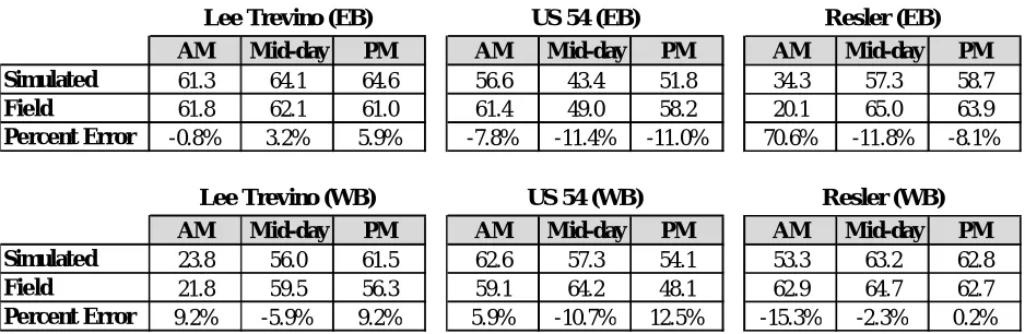
Table 5 is the overall comparison of speeds at all locations and time periods. I-10 at Lee Trevino Dr had the highest degree of accuracy in terms of forecasted speeds on the freeway. During the morning peak hour in the westbound direction, the simulation model was able to forecast speeds within 2 mph. The simulation model was able to at predict speeds at the US 54 interchange to within3.5 mph during the morning peak period. Mid-day comparisons at this location had higher discrepancy but were still within 89% of predicted values.
Table 5: forecasted vs actual Speed Comparison
0 20 40 60 80 0 3 0 0 6 0 0 9 0 0 1 2 0 0 1 5 0 0 1 8 0 0 2 1 0 0 2 4 0 0 2 7 0 0 3 0 0 0 3 3 0 0 3 6 0 0 3 9 0 0 4 2 0 0 4 5 0 0 4 8 0 0 5 1 0 0 5 4 0 0 5 7 0 0 6 0 0 0 6 3 0 0 6 6 0 0 6 9 0 0 7 2 0 0 Sp e e d (m p h ) Time (sec)
Speed Profile (11-1 PM) I-10 @ US 54 EB
Simulated Field 0 20 40 60 80 0 3 0 0 6 0 0 9 0 0 1 2 0 0 1 5 0 0 1 8 0 0 2 1 0 0 2 4 0 0 2 7 0 0 3 0 0 0 3 3 0 0 3 6 0 0 3 9 0 0 4 2 0 0 4 5 0 0 4 8 0 0 5 1 0 0 5 4 0 0 5 7 0 0 6 0 0 0 6 3 0 0 6 6 0 0 6 9 0 0 7 2 0 0 Sp e e d (m p h ) Time (sec)
Speed Profile (11-1 PM) I-10 @ US 54 WB
Simulated Field 0 20 40 60 80 0 30 0 60 0 90 0 12 00 15 00 18 00 21 00 24 00 27 00 30 00 33 00 36 00 39 00 42 00 45 00 48 00 51 00 54 00 57 00 60 00 63 00 66 00 69 00 72 00 Sp ee d (m ph ) Time (sec)
Speed Profile (3-5 PM) I-10 @ Resler EB
Simulated Field 0 20 40 60 80 0 30 0 60 0 90 0 12 00 15 00 18 00 21 00 24 00 27 00 30 00 33 00 36 00 39 00 42 00 45 00 48 00 51 00 54 00 57 00 60 00 63 00 66 00 69 00 72 00 Spe ed (m ph) Time (sec)
Speed Profile (3-5 PM) I-10 @ Resler WB
Simulated Field
AM Mid-day PM AM Mid-day PM AM Mid-day PM
Simulate d 61.3 64.1 64.6 56.6 43.4 51.8 34.3 57.3 58.7
Fie ld 61.8 62.1 61.0 61.4 49.0 58.2 20.1 65.0 63.9
Pe rcent Error -0.8% 3.2% 5.9% -7.8% -11.4% -11.0% 70.6% -11.8% -8.1%
AM Mid-day PM AM Mid-day PM AM Mid-day PM
Simulate d 23.8 56.0 61.5 62.6 57.3 54.1 53.3 63.2 62.8
Fie ld 21.8 59.5 56.3 59.1 64.2 48.1 62.9 64.7 62.7
Pe rcent Error 9.2% -5.9% 9.2% 5.9% -10.7% 12.5% -15.3% -2.3% 0.2% Lee Trevino (EB)
Lee Trevino (WB) US 54 (WB) Resler (WB)
Conclusions
Back casting is a useful and meaningful way of determining the accuracy and validity of forecast model results. It can also be referred to as the last step in the validation process. Modelers can benefit from this methodology by understanding where and why inconsistencies between forecasted and actual results occur. For example, the case study showed that accurate screen line counts (data collection) are a vital part of the calibration process – especially at boundary locations where vehicles enter the network. This case study showed that accurate screen line counts, especially at the boundary locations, are necessary in predicting future traffic patterns, speeds, and travel times.
A MRM approach was used to develop large scale microscopic models for operational planning purposes. However, it must be understood that initial paths and flows are transferred from the mesoscopic to the microscopic level – therefore much effort must be placed in both the initial calibration, but also the consistencies between resolution levels. For example, under-estimating traffic volumes at vehicle loading point locations in the regional mesoscopic model can have a major impact when determining speeds and travel times. It must be noted that this case study was performed for TxDOT with the explicit goal of determining whether speeds in the left most lane on I-10 would improve with the restriction of trucks. In order to conduct a more comprehensive back casting analysis, travel time comparisons between simulated and field data after restrictions are in place is recommended.
In addition, the VoT used in the regional mesoscopic model has an impact on the overall routing assignment thus impacting travel patterns. While the OD was calibrated using data collected in the field, the VoT was held constant against other variables. Further research is needed to assess a more accurate depiction of the VoT for the El Paso region, particularly when assigning vehicles on tolled facilities.
References
Jayakrishnan, R., Simulation of Urban Transportation Networks with Multiple Vehicle Classes and Services: Classification, Functional Requirements and General-Purpose Modeling Schemes, in Annual Meeting of the Transportation Research Board2003, Journal of the Transportation Research Board: Washington D.C. Hawas, Y. and M. Hameed, A multi-stage procedure for validating microscopic traffic simulation models.
Transportation Planning and Technology, 2009. 32(1): p. 7191.
Schiffer, R. and T. Rossi, New Calibration and Validation Standards for Travel Demand Modeling, in Annual Meeting of the Transportation Research Board2008, Journal of the Transportation Research Record: Washington D.C.
Chiu, Y.-C., L. Zhou, and H. Song, Development and calibration of the Anisotropic Mesoscopic Simulation model for uninterrupted flow facilities. Transportation Research Part B: Methodological, 2010. 44(1): p. 152-174. Chiu, Y.C. and J.A. Villalobos, Incorporating Dynamic Traffic Assignment into Long-Range Transportation
Planning with Daily Simulation Assignment and One-Norm Origin-Destination Calibration Formulation. Transportation Research Record Part A: Policy and Practice (under review), 2009.
Chiu, Y.-C., et al. DynusT Online User's Manual. 2009 [cited 2010; Available from: http://dynust.net/wikibin/doku.php?id=start.
Antoniou, C., E. Matsoukis, and P. Roussi, A Methodology for the Estimation of Value-of-Time using State-of-the-Art Econometric Models. Journal of Public Transportation, 2007. Vol 10(3).
Planung Transport Verkehr AG, VISSIM 5.30-05 User Manual, 2011: Karlsruhe, Germany.
Middleton, M., et al., Strategies for Separating Trucks from Passenger Vehicles: Final Report, T.A.M.U. System, Editor 2006, Texas Transportation Institute: College Station.
Kuhn, B., et al., Managed Lane Strategies Feasible for Freeway Ramp Applications: Final Report, 2008, Texas Transportation Institute: College Station.